A fast and robust algorithm to count topologically persistent holes in noisy clouds

Abstract

Preprocessing a 2D image often produces a noisy cloud of interest points. We study the problem of counting holes in noisy clouds in the plane. The holes in a given cloud are quantified by the topological persistence of their boundary contours when the cloud is analyzed at all possible scales.

We design the algorithm to count holes that are most persistent in the filtration of offsets (neighborhoods) around given points. The input is a cloud of $n$ points in the plane without any user-defined parameters. The algorithm has $O(n\log n)$ time and $O(n)$ space. The output is the array (number of holes, relative persistence in the filtration).

We prove theoretical guarantees when the algorithm finds the correct number of holes (components in the complement) of an unknown shape approximated by a cloud.

1 Introduction: counting holes in noisy clouds

We apply methods from the new area of topological data analysis to counting persistent holes in a noisy cloud of points. Such a cloud can be obtained by selecting interest points in a gray scale or RGB image. Our region-based method uses global topological properties of contours.

By a shape we mean any subset $X\subset\mathbb{R}^{2}$ that can be split into finitely many (topological) triangles. Hence $X$ is bounded, but may not be connected. Then a hole in a shape $X\subset\mathbb{R}^{2}$ is a bounded connected component of the complement $\mathbb{R}^{2}-X$. Such a hole can be a disk, a ring or may have a more complicated topological form, see Fig. 1.

Figure 1: The orange shape $X\subset\mathbb{R}^{2}$ with 3 white holes of different forms: a small disk, a ring-like hole, a ‘figure-eight’ hole.

The $\alpha$-offset $X^{\alpha}$ is the union $\cup_{p\in X}B(p;\alpha)$ of disks with the radius $\alpha\geq 0$ and centers at all $p\in X$. For instance, $X^{0}$ is the original shape $X\subset\mathbb{R}^{2}$. When $\alpha$ is increasing, the holes of $\mathbb{R}^{2}-X^{\alpha}$ are shrinking, may split into smaller newborn holes and will eventually die, each at its own death time $\alpha$, see Fig. 3. The persistence of a hole is its life span $\mathrm{death}-\mathrm{birth}$ in the filtration $\{X^{\alpha}\}$ of all $\alpha$-offsets. So we quantify holes by their persistence at different scales $\alpha$.

Hole counting problem. Let a shape $X$ be represented by a finite sample $C$ of points in $\mathbb{R}^{2}$. Find conditions on $X$ and its sample when one can quickly count persistent holes.

We solve the problem by the algorithm HoCToP : Hole Counting based on Topological Persistence. The only input is a finite cloud $C$ of $n$ points approximating an unknown shape $X\subset\mathbb{R}^{2}$. The algorithm outputs the relative persistence of $k$ holes in the filtration $\{C^{\alpha}\}$ for all $k\geq 0$. If the scale $\alpha$ is random and uniform, this output gives probabilities $P(k\mbox{ holes})$. The boundary edges of persistent holes can be quickly post-processed to extract all boundary contours.

Figure 2: Input: cloud $C$ of 1251 points uniformly sampled from the shape with 3 holes in Fig. 1. Output probabilities of HoCToP : $P(\mbox{3 holes})\approx 24\%$, $P(\mbox{2 holes})\approx 13\%$, $P(\mbox{8 holes})\approx 11\%$.

Theorems 1, 4 say that the algorithm HoCToP quickly and correctly finds all persistent holes using only a good enough sample $C$ of an unknown shape $X$, see section 2.

2 Main results: the algorithm and guarantees

We start from a high-level description of our algorithm.

The topological persistence of contours in the filtration $\{C^{\alpha}\}$ is computed by using a Delaunay triangulation $\mathrm{Del}(C)$ of a given cloud $C\subset\mathbb{R}^{2}$ of $n$ points. By Nerve Lemma 8 the $\alpha$-offsets $C^{\alpha}$ can be continuously deformed to the $\alpha$-complexes $C(\alpha)$, which filter $\mathrm{Del}(C)$ as follows:
$C=C(0)\subset\dots\subset C(\alpha)\subset\dots\subset C(+\infty)=\mathrm{Del}(C)$. Each $C(\alpha)$ has some edges and triangles from $\mathrm{Del}(C)$.

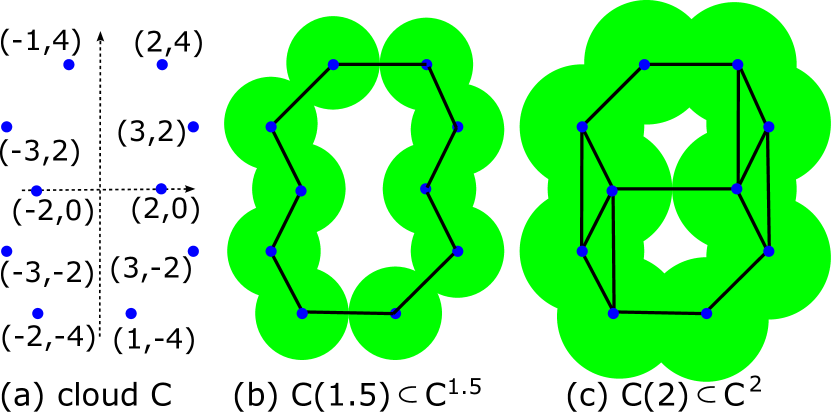
Figure 3: The big hole in the green offset $C^{\alpha}$ is born at $\alpha=1.5$, splits into 2 smaller holes at $\alpha=2$ and dies at $\alpha\approx 2.577$, so the topological persistence of this hole is $\mathrm{death}-\mathrm{birth}\approx 1.077$.

The graph dual to $\mathrm{Del}(C)$ is filtered by the subgraphs $C^{*}(\alpha)$ whose connected components correspond to holes in $C(\alpha)$. When $\alpha$ is decreasing, $C(\alpha)$ is shrinking, so its holes are growing and corresponding components of $C^{*}(\alpha)$ merge at critical values of $\alpha$, see Fig. 6. The persistence of cycles in the filtration $\{C^{\alpha}\}$ corresponds to the persistence of components in $\{C^{*}(\alpha)\}$, see Duality Lemma 14.

The pairs $(\mathrm{birth},\mathrm{death})$ of connected components in $\{C^{*}(\alpha)\}$ are found via a union-find structure by adding edges and merging components. So computing the 1-dimensional persistence of cycles in $\{C^{\alpha}\}$ reduces to the 0-dimensional persistence of components in $\{C^{*}(\alpha)\}$.

Starting from a given cloud $C\subset\mathbb{R}^{2}$ of $n$ points with real coordinates $(x_{i},y_{i})$, $i=1,\dots,n$, we find a Delaunay triangulation $\mathrm{Del}(C)$ in $O(n\log n)$ time with $O(n)$ space. Then we remove each edge of $\mathrm{Del}(C)$ one by one in the decreasing order of their length. Removing an edge may break a contour when adjacent regions in $C(\alpha)$ and the corresponding components of $C^{*}(\alpha)$ merge. In the case of a merger, a younger component of $C^{*}(\alpha)$ and the corresponding hole in $C(\alpha)$ die. We note the $\mathrm{birth}$ and $\mathrm{death}$ of each dead hole. We get the probability of $k$ holes as the relative length of all intervals of the scale $\alpha$ when $C^{\alpha}\subset\mathbb{R}^{2}$ has $k$ holes.

Theorem 1.

The algorithm HoCToP  counts all holes in a given cloud $C\subset\mathbb{R}^{2}$ of $n$ points in $O(n\log n)$ time with $O(n)$ space. All holes are ordered by their topological persistence in the ascending filtration $\{C^{\alpha}\}$ of the $\alpha$-offsets.

Definition 2 ($\varepsilon$-sample).

A cloud $C$ is an $\varepsilon$-sample of a shape $X\subset\mathbb{R}^{2}$ if $X\subset C^{\alpha}$ and $C\subset X^{\alpha}$. So any point of $C$ is within the distance $\varepsilon$ from a point of $X$ and any point of $X$ is at most $\varepsilon$ away from a point of $C$. Hence $\varepsilon$ can be considered as the upper bound of some arbitrary noise.

Definition 3 (min and max homological feature sizes).

For any shape $X\subset\mathbb{R}^{2}$, let $\alpha=\mathrm{minhfs}(X)$ be the minimum homological feature size when a first hole is born or dies in $X^{\alpha}$. Let $\alpha=\mathrm{maxhfs}(X)$ be the maximum homological feature size after which no holes are born or die in $X^{\alpha}$.

Theorem 4 gives sufficient (not necessary) conditions when the algorithm finds the correct number of holes in an unknown shape $X\subset\mathbb{R}^{2}$ that is represented by its finite sample $C$. We extend the Homology Inference Theorem [4] to the case when the upper bound $\varepsilon$ of noise is unknown.

Theorem 4.

Let a cloud $C$ be an $\varepsilon$-sample of a shape $X\subset\mathbb{R}^{2}$ with an unknown parameter $\varepsilon$ such that $\mathrm{minhfs}(X)>\frac{1}{2}\mathrm{maxhfs}(X)+4\varepsilon$. If no new holes are appear in $X^{\alpha}$ when $\alpha$ is increasing, then the algorithm HoCToP  finds the correct number of holes in $X$ by using only the cloud $C$.

The condition $\mathrm{minhfs}(X)>\frac{1}{2}\mathrm{maxhfs}(X)+4\varepsilon$ means that all holes of $X$, which are bounded components of $\mathbb{R}^{2}-X$, have comparable sizes (neither tiny nor huge).

Even if the conditions of Theorem 4 are not satisfied, we can always find the number $k$ of holes with the highest probability. The algorithm HoCToP  can also accept a signal-to-noise ratio $\tau$ and output all holes whose persistence is larger than $\tau$. Alternatively, the user may prefer to get most likely outputs ordered by the probability $P(k\mbox{ holes})$.

3 Previous work on computing persistence

The offsets $C^{\alpha}$ of a finite cloud $C$ are usually studied through the C̆ech or Rips complexes, which may contain up to $O(n^{k})$ simplices in all dimensions $k\leq n-1$ even if $C\subset\mathbb{R}^{2}$. A Delaunay triangulation has the advantage of a smaller size up to $m=O(n^{2})$ in dimensions $n=2,3,4$.

The fastest algorithm [8] for computing persistence of a filtration in all dimensions has the same running time $O(m^{2.376})$ in the number $m$ of simplices as the best known time for the multiplication of two $m\times m$ matrices.

In dimension 0 the persistence can be computed in almost linear time [6, p. 6–8], which was used for simplifying functions on surfaces [1] and for approximating persistence of an unknown scalar field from its values on a sample [3].

Two extra parameters were used in a Delaunay-based image segmentation [7]: $\alpha$ for the radius of disks centered at points of a cloud $C$ and $p$ for a desired level of persistence.

4 Delaunay triangulation and $\alpha$-complexes

Definition 5 (simplicial complex).

A simplicial 2-complex is a finite set of simplices (vertices, edges, triangles):

$\bullet$ the sides of any triangle are included in the complex;

$\bullet$ the endpoints of any edge are included in the complex;

$\bullet$ two triangles can intersect only along a common edge;

$\bullet$ edges can meet only at a common endpoint (a vertex);

$\bullet$ an edge can not pierce through the interior of a triangle.

If a complex $S$ is drawn in $\mathbb{R}^{n}$ without self-intersections, we may call this image $|S|$ a geometric realization of $S$. We have defined a shape $X\subset\mathbb{R}^{2}$ as a geometric realization of a 2-complex. For instance, a round disk whose boundary is split into 3 edges by 3 vertices is a topological triangle.

A cycle in a complex is a sequence of edges $e_{1},\dots,e_{m}$ such that any consecutive edges $e_{i},e_{i+1}$ (in the cyclic order) have a common vertex. Any loop in a geometric realization $|S|$ continuously deforms to a cycle of edges in $S$.

Definition 6 (Delaunay triangulation $\mathrm{Del}$).

For a point $p_{i}$ in a cloud $C=\{p_{1},\dots,p_{n}\}\subset\mathbb{R}^{2}$, the Voronoi cell $V(p_{i})=\{q\in\mathbb{R}^{2}:d(p_{i},q)\leq d(p_{j},q)\;\forall j\neq i\}$ is the set of all points $q$ that are (non-strictly) closer to $p_{i}$ than to other points of $C$. The Delaunay triangulation $\mathrm{Del}(C)$ is the nerve of the Voronoi diagram $\cup_{p\in C}V(p)$. Namely, $p,q,r\in C$ span a triangle if and only if $V(p)\cap V(q)\cap V(r)\neq\emptyset$.

By another definition [2, section 9.1] the circumcircle of any Delaunay triangle in $\mathrm{Del}(C)$ encloses no points of $C$.

For a cloud $C\subset\mathbb{R}^{2}$ of $n$ points, let $\mathrm{Del}(C)$ have $k$ triangles and $b$ boundary edges in the external region. Counting all $E$ edges over triangles, we get $3k+b=2E$. Euler’s formula $n-E+(k+1)=2$ implies that $k=2n-b-2$, $E=3n-b-3$. So $\mathrm{Del}(C)$ has $O(n)$ edges and triangles.

Definition 7 ($\alpha$-complex $C(\alpha)$).

For a scale parameter $\alpha>0$, the $\alpha$-complex $C(\alpha)$ is the nerve of $\cup_{p\in C}(V(p)\cap B(p;\alpha))$, see [6, section III.4]. Points $p,q\in C$ are connected by an edge if $V(p)\cap B(p;\alpha)$ meets $V(q)\cap B(q;\alpha)$. Three points $p,q,r\in C$ span a triangle if the intersection $V(p)\cap B(p;\alpha)\cap V(q)\cap B(q;\alpha)\cap V(r)\cap B(r;\alpha)\neq\emptyset$.

If $\alpha>0$ is very small, all points of $C$ are disjoint in $C(\alpha)$, while $C(\alpha)=\mathrm{Del}(C)$ for any large enough $\alpha$, see examples in Fig. 3. So all $\alpha$-complexes form the filtration $C=C(0)\subset\dots\subset C(\alpha)\subset\dots\subset C(+\infty)=\mathrm{Del}(C)$. Edges or triangles are added only at critical values of $\alpha$.

Lemma 8 (Nerve of a ball covering [5]).

The union of balls $C^{\alpha}=\cup_{p\in C}B(p;\alpha)$ continuously deforms to (has the homotopy type of) a geometric realization of $C(\alpha)$.

5 Persistent homology: definitions, examples

Definition 9 (1-dimensional homology $H_{1}$).

We consider the 1-dimensional homology group $H_{1}(S)$ only with coefficients in $\mathbb{Z}/2\mathbb{Z}=\{0,1\}$. Cycles of a 2-dimensional complex $S$ can be algebraically written as linear combinations of edges (with coefficients $0$ or $1$) and generate the vector space $C_{1}$ of cycles. The boundaries of all triangles in $S$ (as cycles of 3 edges) generate the subspace $B_{1}\subset C_{1}$. The quotient group $C_{1}/B_{1}$ is the homology group $H_{1}(S)$.

By a filtration $\{S(\alpha)\}$ we mean a sequence of nested complexes $S(0)\subset\dots\subset S(\alpha)\subset\dots$ that change only at finitely many critical values $\alpha_{1},\dots,\alpha_{m}$. Then we get the induced linear maps $H_{1}(S(\alpha_{1}))\to\dots\to H_{1}(S(\alpha_{m}))$.

Definition 10 (persistence diagram $\mathrm{PD}\{S(\alpha)\}$).

In a filtration $\{S(\alpha)\}$ a homology class $\gamma\in H_{1}(S(\alpha_{i}))$ is born at $\alpha_{i}=\mathrm{birth}(\gamma)$ if $\gamma$ is not in the image of $H_{1}(S(\alpha))\to H_{1}(S(\alpha_{i}))$ for any $\alpha<\alpha_{i}$. The class $\gamma$ dies at the first time $\alpha_{j}=\mathrm{death}(\gamma)\geq\alpha_{i}$ when the image of $\gamma$ under $H_{1}(S(\alpha_{i}))\to H_{1}(S(\alpha_{j}))$ merges into the image of $H_{1}(S(\alpha))\to H_{1}(S(\alpha_{j}))$ for some $\alpha<\alpha_{i}$. The class $\gamma$ has the persistence $\mathrm{death}(\gamma)-\mathrm{birth}(\gamma)$. The point $(\alpha_{i},\alpha_{j})$ has the multiplicity $\mu_{ij}$ equal to the number of independent classes that are born at $\alpha_{i}$ and die at $\alpha_{j}$. The persistence diagram $\mathrm{PD}\{S(\alpha)\}$ in $\{(x,y)\in\mathbb{R}^{2}:x\leq y\}$ is the multi-set consisting of all points $(\alpha_{i},\alpha_{j})$ with the multiplicity $\mu_{ij}$ and all diagonal points $(x,x)$ with the infinite multiplicity.

Pairs with a low persistence $\mathrm{death}-\mathrm{birth}$ (close to the diagonal $\{x=y\}$ in $\mathrm{PD}$) are treated as noise. Pairs with a high persistence represent persistent cycles in $\{S(\alpha)\}$.

We shall consider the filtrations of $\alpha$-offsets $\{X^{\alpha}\}$ and $\{C^{\alpha}\}$ for a shape $X\subset\mathbb{R}^{2}$ and a finite cloud $C\subset\mathbb{R}^{2}$. Figures 4 and 5 show the persistence diagram $\mathrm{PD}$ for the filtration of the $\alpha$-offsets $C^{\alpha}$ equivalent to $C(\alpha)$ by Lemma 8.

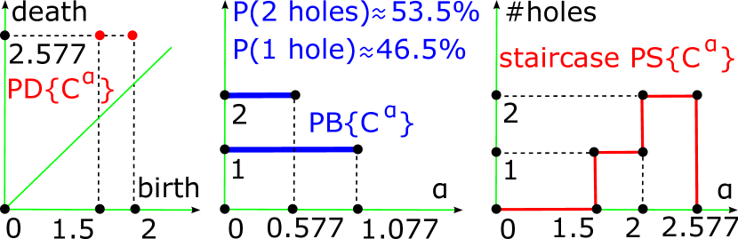
Figure 4: Extra outputs for the cloud $C$ of 10 points in Fig. 3. Left: persistence diagram, middle: barcode, right: persistence staircase.

We can convert the persistence diagram into the persistence barcode $\mathrm{PB}\{C^{\alpha}\}$. All pairs $(\mathrm{birth},\mathrm{death})$ give horizontal bars ordered by their length $\mathrm{death}-\mathrm{birth}$. Usually the bars are drawn from the left endpoint $0$ to the right endpoint $\mathrm{death}-\mathrm{birth}$, see the middle picture in Fig. 4.

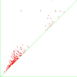
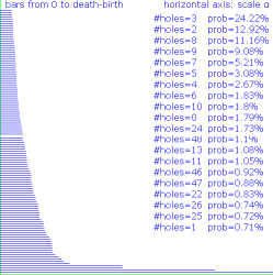
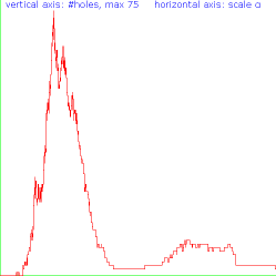
Figure 5: Extra outputs for the cloud $C$ of 1251 points in Fig. 2. Left: persistence diagram $\mathrm{PD}$, middle: barcode $\mathrm{PB}$, right: staircase $\mathrm{PS}$.

We suggest one more way to visualize persistence. Each pair $(\mathrm{birth},\mathrm{death})$ defines the function $f(\alpha)=1$ for $\mathrm{birth}\leq\alpha<\mathrm{death}$ and $f(\alpha)=0$ otherwise. The sum of these functions over all pairs gives the persistence staircase $\mathrm{PS}\{C^{\alpha}\}$. The value of this piecewise constant function of $\alpha$ is the number of holes in the offset $C^{\alpha}$. We have connected consecutive horizontal segments of $\mathrm{PS}\{C^{\alpha}\}$ to get a ‘continuous’ staircase as in the right picture of Fig. 4.

For the cloud $C$ of 10 points in Fig. 3, the full range of the scale $\alpha$ is from the smallest critical value $\alpha=1.5$ (when a first hole is born) to the largest critical value $\alpha=\frac{5}{8}\sqrt{17}\approx 2.577$ (when both final holes die). The output probability $P(\mbox{1 hole})\approx 46.5\%$ is the contribution of the interval $(1.5,2)$ to the full range $1.5\leq\alpha\leq\frac{5}{8}\sqrt{17}$. The largest probability $P(\mbox{2 holes})\approx 53.5\%$ is the contribution of the interval $(2,\frac{5}{8}\sqrt{17})$ when $C^{\alpha}$ has exactly 2 holes.

For the cloud $C$ of 1251 points in Fig. 2, we scaled $\mathrm{PB}\{C^{\alpha}\}$ and $\mathrm{PS}\{C^{\alpha}\}$ along the horizontal $\alpha$-axis and kept only the longest bars in the barcode $\mathrm{PB}\{C^{\alpha}\}$ in Fig. 5.

6 Persistent homology: stability and duality

Definition 11 (bottleneck distance $d_{B}$).

Let the distance between $p=(x_{1},y_{1})$, $q=(x_{2},y_{2})$ in $\mathbb{R}^{2}$ be $||p-q||_{\infty}=\max\{|x_{1}-x_{2}|,|y_{1}-y_{2}|\}$. The bottleneck distance is $d_{B}(D,D^{\prime})=\inf_{\varphi}\sup_{p\in D}||p-\varphi(p)||_{\infty}$ over all bijections $\varphi:D\to D^{\prime}$ between persistence diagrams $D,D^{\prime}$.

Theorem 12.

[4] If a finite cloud $C$ of points is an $\varepsilon$-sample of a shape $X\subset\mathbb{R}^{2}$, then $d_{B}(\mathrm{PD}\{X^{\alpha}\},\mathrm{PD}\{C^{\alpha}\})\leq\varepsilon$.

Stability Theorem 12 implies for barcodes $\mathrm{PB}$ that the endpoints of all bars are perturbed by at most $\varepsilon$. So a long bar can become only a bit shorter after adding noise.

To every triangle in the Delaunay triangulation $\mathrm{Del}(C)$, let us associate a single abstract vertex $v_{i}$, $i=1,\dots,k$. It will be convenient to call the external region of $\mathrm{Del}(C)$ also a ‘triangle’ and represent it by an extra vertex $v_{0}$.

Definition 13 (graphs $C^{*}(\alpha)$).

For any vertices $v_{i},v_{j}$ representing adjacent triangles in $\mathrm{Del}(C)$, let $d_{ij}$ be the length of the (longest) common edge of the triangles. The metric graph $C^{*}$ dual to $\mathrm{Del}(C)$ has the vertices $v_{0},v_{1},\dots,v_{k}$ and edges of the length $d_{ij}$ connecting vertices $v_{i},v_{j}$ that represent adjacent triangles, see Fig. 6. The graph $C^{*}$ is filtered by the subgraphs $C^{*}(\alpha)$ that have only the edges of a length $d_{ij}>2\alpha$. We remove any isolated node $v$ (except $v_{0}$) from $C^{*}(\alpha)$ if the corresponding triangle $T_{v}$ is not acute or has a small circumradius $\mathrm{rad}(v)\leq\alpha$. We get the filtration $C^{*}=C^{*}(0)\supset\dots\supset C^{*}(\alpha)\supset\dots\supset C^{*}(+\infty)=\{v_{0}\}$.

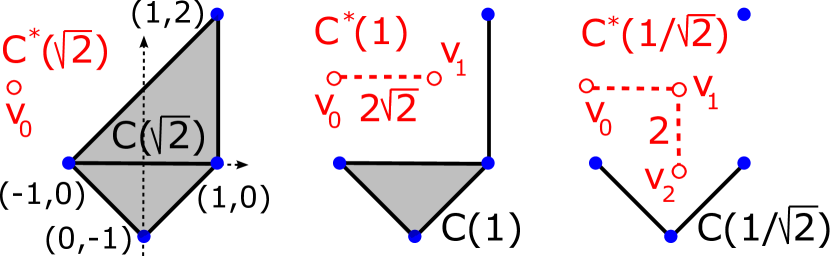
Figure 6: The complexes $C(\alpha)$ have solid edges and gray triangles. The graphs $C^{*}(\alpha)$ have circled vertices and red dashed edges.

Components of $C^{*}(\alpha)$ are called white, because they represent regions in $\mathbb{R}^{2}-C(\alpha)$ (or holes in $\mathbb{R}^{2}-C^{\alpha}$). A cycle $\gamma\subset C(\alpha)$ is called a contour if $\gamma$ bounds a region in $\mathbb{R}^{2}-C(\alpha)$, so $\gamma$ ‘encloses’ the corresponding white component of $C^{*}(\alpha)$. Lemma 14 is an analogue of the Symmetry Theorem [6, p. 164] for a function on a closed manifold.

Lemma 14 (Duality).

All contours of the complex $C({\alpha})$ are in a 1-1 correspondence with all connected components of the graph $C^{*}(\alpha)$ not containing the vertex $v_{0}$. When $\alpha$ is decreasing, the contours of $C(\alpha)$ and the white components of $C^{*}(\alpha)$ have the corresponding critical moments:

$\bullet$ a birth of a contour $\leftrightarrow$ a birth of a white component,

$\bullet$ a death of a contour $\leftrightarrow$ a death of a white component. ∎

7 The algorithm HoCToP for counting holes

We build the union-find structure $\mathrm{Forest}(\alpha)$ on the vertices of the graph $C^{*}(\alpha)$. All nodes and trees of $\mathrm{Forest}(\alpha)$ will be in a 1-1 correspondence with all vertices and white components of $C^{*}(\alpha)$. Every node $v$ in $\mathrm{Forest}(\alpha)$ has

$\bullet$ a pointer to a unique parent of the node $v$ in $\mathrm{Forest}(\alpha)$;

$\bullet$ a pointer to the Delaunay triangle dual to the node $v$;

$\bullet$ the weight (the number of nodes below $v$ in its tree);

$\bullet$ the critical value (birth) $\alpha_{v}=\sup\{\alpha:v\in C^{*}(\alpha)\}$.

If a node $v$ is a self-parent, we call $v$ a root. We can find $\mathrm{root}(v)$ of any node $v$ by going up along parent links. If $\alpha$ is decreasing, $\alpha_{v}$ can be considered as the birth time when the vertex $v$ joins $C^{*}(\alpha)$. The algorithm initializes $\mathrm{Forest}(\alpha)$ as the set of isolated nodes $v_{0},\dots,v_{k}$. If the triangle corresponding to $v_{k}$ is acute, the birth time of $v_{k}$ is the circumradius of the triangle, otherwise 0. We will go through all edges of $\mathrm{Del}(C)$ in the decreasing order of their length and will update $\alpha_{v}$ when $v$ enters the ascending filtration $\{v_{0}\}=C^{*}(+\infty)\subset\dots\subset C^{*}(\alpha)\subset\dots\subset C^{*}(0)=C^{*}$.

All triangles of $C(\alpha)$ and the corresponding nodes of $\mathrm{Forest}(\alpha)$ are called gray. The remaining triangles and the external region of $\mathrm{Del}(C)$ are called white. The external region has birth time $+\infty$ and is called a ‘triangle’ for simplicity. Initially all triangles with birth time 0 are gray.

The while loop. For each edge $e\subset\mathrm{Del}(C)$ arriving in the decreasing order of length, we find two triangles $T_{u},T_{v}$ attached to $e$ and check if they are gray or white. To determine if a triangle $T_{v}$ represented by a node $v$ is gray, we go up along parent links from $v$ to $\mathrm{root}(v)$. If the birth time of $\mathrm{root}(v)$ is 0, the triangle $T_{v}$ is still gray, otherwise white.

To distinguish Cases 1 and 4 below, we also check if the triangles $T_{u},T_{v}$ attached to the current edge $e$ are in the same region of $\mathbb{R}^{2}-C(\alpha)$. Case 1 means that the nodes $u,v\in\mathrm{Forest}(\alpha)$ belong to the same tree, so $\mathrm{root}(u)=\mathrm{root}(v)$. In all 4 cases the scale $\alpha$ goes down through the half-length $\frac{1}{2}\mathrm{length}(e)$ of the current edge $e$ from $\mathrm{Del}(C)$.

Case 1: $e$ has the same white region on both sides of $e$.

$C(\alpha)$ loses only the open edge $e$. The white components of $C^{*}(\alpha)$ are unchanged. Fig. 6 illustrates Case 1 for $\alpha=1$ when $C(\alpha)$ loses the edge connecting $(1,0)$ to $(1,2)$.

Case 2: the edge $e$ is in 1 gray triangle and 1 white triangle.

Let $u,v\in C^{*}(\alpha)$ be the vertices dual to the gray triangle $T_{u}$ and the white triangle $T_{v}$ attached to the current edge $e$ in $\mathrm{Del}(C)$. Then the birth times are $\alpha_{u}=0$, $\alpha_{\mathrm{root}(v)}>0$.

Since $\alpha$ is decreasing, the descending filtration $C(\alpha)$ loses the (open) edge $e$ and the gray (open) triangle $T_{u}$. So the vertex $u$ becomes connected by an edge with $v$ and joins the white component of $C^{*}(\alpha)$ containing $v$. Then we link the isolated node $u$ to the tree containing the older node $v$ in $\mathrm{Forest}(\alpha)$. So $\mathrm{root}(v)$ becomes the parent of $u$ and the weight of $\mathrm{root}(v)$ jumps by 1. Fig. 7 illustrates Case 2 for $\alpha=\frac{\sqrt{17}}{2}$ when $C(\alpha)$ loses the 2 edges of length $\sqrt{17}$.

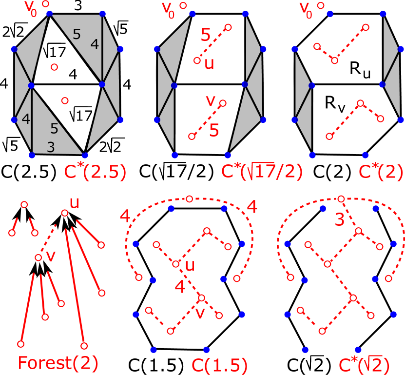
Figure 7: Complexes $C(\alpha)$ and graphs $C^{*}(\alpha)$ are shown for the cloud $C$ from Fig. 3. Two trees in $\mathrm{Forest}(\alpha)$ merge at $\alpha=2$.

Case 3: the edge $e$ is in the boundary of 2 gray triangles.

Let $u,v\in C^{*}(\alpha)$ be the vertices dual to the gray triangles $T_{u},T_{v}$ attached to the current edge $e\subset\mathrm{Del}(C)$. Then $T_{u},T_{v}$ are right-angled triangles with the common hypotenuse $e$. The birth time of both $u,v$ is the half-length of $e$. Since $\alpha$ is decreasing, $C(\alpha)$ loses the (open) edge $e$ and both (open) triangles $T_{u},T_{v}$. The contour $\partial(T_{u}\cup T_{v})$ appears in $C(\alpha)$. So we link the nodes $u,v$ in $\mathrm{Forest}(\alpha)$.

Case 4: $e$ has 2 different white regions on both sides.

Let $u,v\in C^{*}(\alpha)$ be the vertices dual to the white triangles $T_{u},T_{v}$ attached to the current edge $e$ in $\mathrm{Del}(C)$. The descending filtration $\{C(\alpha)\}$ loses the (open) edge $e$. The vertices $u,v$ become connected by an edge, so their white components in $C^{*}(\alpha)$ merge into a new big component. By Duality Lemma 14, two contours enclosing regions $R_{u}$ and $R_{v}$ lose their common edge $e$ and we get one larger contour $\partial(R_{u}\cup R_{v})$ enclosing both regions. Fig. 7 illustrates Case 4 for $\alpha=2$ when $C(\alpha)$ loses the middle edge of length 4. Then 2 white components (containing 4 vertices each) merge in the graph $C^{*}(\alpha)$ shown after merger at $\alpha=1.5$.

To decide which white component dies, we find the roots $\mathrm{root}(u),\mathrm{root}(v)\in\mathrm{Forest}(\alpha)$ of the trees representing $R_{u},R_{v}$ and compare the birth times $\alpha_{\mathrm{root}(u)},\alpha_{\mathrm{root}(v)}$ when a first node of each tree was born. By the elder rule [6, p. 150], the older white component (say, with $u$) survives and keeps its larger birth time $\alpha_{\mathrm{root}(u)}$. The younger white component $R_{v}$ dies and we get $(\mathrm{birth},\mathrm{death})=(\frac{1}{2}\mathrm{length}(e),\alpha_{\mathrm{root}(v)})$ for the life of the white component in the ascending filtration $\{C^{*}(\alpha)\}$ and of the corresponding contour in the descending filtration $\{C(\alpha)\}$.

We swapped the birth and death times, because the persistence is usually defined when the scale $\alpha$ is increasing. However, we need the ascending filtration $\{C^{*}(\alpha)\}$ to use a union-find structure, so $\alpha$ is decreasing in the algorithm.

Finally, to merge the trees with $\mathrm{root}(u),\mathrm{root}(v)$ in $\mathrm{Forest}(\alpha)$, we compare the weights of the roots and set the root of the (non-strictly) larger tree as the parent for the root of another tree. So the size of any subtree grows by a factor of at least 2 each time when we pass to the parent. We get

Lemma 15.

By the above construction the longest path in any tree of size $k$ from $\mathrm{Forest}(\alpha)$ has length $O(\log k)$. ∎

8 Proofs of main results and our conclusion

Proof of Theorem 1. Constructing the Delaunay triangulation $\mathrm{Del}(C)$ on a cloud of $n$ points requires $O(n\log n)$ time [2, Chapter 9]. Sorting $O(n)$ edges of $\mathrm{Del}(C)$ needs $O(n\log n)$ time. Then we go through the while loop analyzing each of the $O(n)$ edges of $\mathrm{Del}(C)$. For the nodes $u,v\in\mathrm{Forest}(\alpha)$ of triangles attached to each edge $e$, we find the roots of $u,v$ by going up along $O(\log n)$ parent links by Lemma 15. All other steps in the while loop require only $O(1)$ time. Hence the total time is $O(n\log n)$. The sizes of all data structures are proportional to the numbers of edges or triangles in $\mathrm{Del}(C)$, so we use $O(n)$ space. ∎

The careful analysis of a union-find structure says that $\mathrm{Forest}(\alpha)$ can be built in time $O(nA^{-1}(n,n))$ time, where $A^{-1}(n,n)$ is the extremely slowly growing inverse Ackermann function. Our time $O(n\log n)$ is dominated by the construction of $\mathrm{Del}(C)$ and sorting all $O(n)$ edges.

Proof of Theorem 4. The important critical values of $\alpha$ for the 1-dimensional homology of the filtration $\{X^{\alpha}\}$ are

$\bullet$ $\alpha=\mathrm{minhfs}(X)$ is the 1st value when $H_{1}(X^{\alpha})$ changes;

$\bullet$ $\alpha=\mathrm{maxhfs}(X)$ is the last value when $H_{1}(X^{\alpha})$ changes.

No new holes appear in offsets $X^{\alpha}$ of the shape $X$ with original $k$ holes. Then $\mathrm{PD}\{X^{\alpha}\}$ contains only points $(0,d_{i})$. The smallest death is $d_{1}=\mathrm{minhfs}(X)$. The largest death is $d_{k}=\mathrm{maxhfs}(X)$. If a cloud $C$ is an $\varepsilon$-sample of a shape $X\subset\mathbb{R}^{2}$, the perturbed diagram $\mathrm{PD}\{C^{\alpha}\}$ has only points $\varepsilon$-close to $(0,d_{i})$ or to the diagonal $\{x=y\}$ in the $L_{\infty}$ distance on the plane by Stability Theorem 12.

The strip $\{2\varepsilon<y-x<d_{1}-2\varepsilon\}$ is the largest empty strip in $\mathrm{PD}\{C^{\alpha}\}$ due to the given condition $d_{1}>\frac{1}{2}d_{k}+4\varepsilon$ or $(d_{1}-2\varepsilon)-2\varepsilon>(d_{k}+2\varepsilon)-(d_{1}-2\varepsilon)$. Then we can detect this strip in $\mathrm{PD}\{C^{\alpha}\}$ without using $\varepsilon$. Hence $\mathrm{PD}\{C^{\alpha}\}$ has exactly $k$ points above $y-x=d_{1}-2\varepsilon$ close to $(0,d_{i})$ corresponding to $k$ holes of the unknown shape $X$. ∎

Conclusion. Here are the key advantages of our approach:

$\bullet$ a cloud $C\subset\mathbb{R}^{2}$ of $n$ points is simultaneously analyzed at all scales $\alpha$ without any extra user-defined parameters;

$\bullet$ the algorithm HoCToP counts persistent holes of any topological form in $O(n\log n)$ time, see Theorem 1;

$\bullet$ theoretical guarantees for a correct number of holes are proved for $\varepsilon$-samples of unknown shapes, see Theorem 4;

$\bullet$ the output is stable under perturbations of a cloud $C$ and the only parameter of noise is an unknown upper bound $\varepsilon$.

Fig. 8 shows extracted contours (with our uniform noise) of images at http://www.lems.brown.edu/~dmc.

Figure 8: Output of HoCToP   for real noisy contours. Left: $P(\mbox{1 hole})\approx 90.5\%$, $P(\mbox{2 holes})\approx 3\%$, $P(\mbox{4 holes})\approx 0.6\%$. Right: $P(\mbox{2 holes})\approx 74.2\%$, $P(\mbox{1 hole})\approx 13\%$, $P(\mbox{3})\approx 1.3\%$.

More details, code, experiments are at author’s website http://kurlin.org. We thank reviewers for helpful comments and are open to collaboration on related projects.

Appendix A: a pseudo-code of HoCToP 

Algorithm 1 below contains the pseudo-code of the our main algorithm HoCToP . Cases 2–4 from the description in section 7 are covered in further Algorithms 2–4.

Algorithm 1 Find $(\mathrm{birth},\mathrm{death})$ of all cycles in $C(\alpha)$

0:  a cloud $C$ given as pairs $(x_{1},y_{1}),\dots(x_{n},y_{n})$

1:  Build Delaunay triangulation $\mathrm{Del}(C)$ with $k$ triangles

2:  Extract all edges with pointers to 2 adjacent triangles

3:  Sort edges of $\mathrm{Del}(C)$ in the decreasing order of length

4:  $\mathrm{Forest}\leftarrow$ isolated nodes $v_{0},\dots,v_{k}$ with birth times $0$

5:  For the external node $v_{0}$, update the birth $\alpha\leftarrow+\infty$

6:  For each acute triangle $T_{v}$, $\alpha_{v}\leftarrow$ circumradius of $T_{v}$

7:  Set the total number of links in $\mathrm{Forest}(\alpha)$: $L\leftarrow 0$

8:  while $L<k$ (we stop when $\mathrm{Forest}(\alpha)$ is a tree) do

9:     Take the next longest edge $e$ from $\mathrm{Del}(C)$

10:     Set the current critical value: $\alpha\leftarrow\frac{1}{2}\mathrm{length}(e)$

11:     Find 2 nodes $u,v$ dual to the triangles attached to $e$

12:     Find the roots $\mathrm{root}(u),\mathrm{root}(v)$ of the nodes $u,v$

13:     if $\mathrm{root}(u)=\mathrm{root}(v)$ ($u,v$ in the same region) then

14:        Case 1 (no changes): continue the while loop

15:     else if $\alpha_{\mathrm{root}(u)}=0$ and $\alpha_{\mathrm{root}(v)}>0$ then

16:        Case 2 ($u$ gray, $v$ white): run Algorithm 2

17:     else if $\alpha_{\mathrm{root}(u)}=0$ and $\alpha_{\mathrm{root}(v)}=0$ then

18:        Case 3 (both $u,v$ are gray): run Algorithm 3

19:     else

20:        Case 4 ($\alpha_{\mathrm{root}(u)},\alpha_{\mathrm{root}(v)}>0$): run Algorithm 4

21:     end if

22:     $L\leftarrow L+1$ (one link was added in Cases 2, 3, 4)

23:  end while

24:  return  array of pairs $(\mathrm{birth},\mathrm{death})$ from Case 4

Recall that a node $u$ is gray if the birth time $\alpha_{u}=0$. The case ($u$ white, $v$ gray) is symmetric to Case 2 below, so we simply denote the gray node by $u$ when calling Algorithm 2.

Algorithm 2 Link 2 nodes $u,v$ in $\mathrm{Forest}(\alpha)$ in Case 2

0:  nodes $u$ and $\mathrm{root}(v)$ (so $u$ is gray, $v$ is white)

1:  Set $\mathrm{root}(v)$ as parent of $u$, set $\alpha_{u}\leftarrow\alpha_{\mathrm{root}(v)}$

2:  Add 1 (coming from $u$) to the weight of $\mathrm{root}(v)$

In Algorithm 3 below any of the gray nodes $u,v$ can be the parent of the other node, we have simply chosen $u$.

Algorithm 3 Link 2 nodes $u,v$ in $\mathrm{Forest}(\alpha)$ in Case 3

0:  $\alpha$, nodes $u,v$ dual to triangles (both $u,v$ gray)

1:  Set $u$ as the parent of the node $v$ in $\mathrm{Forest}(\alpha)$

2:  Set: $\alpha_{u},\alpha_{v}\leftarrow\alpha$, $\mathrm{weight}(u)\leftarrow 1$, $\mathrm{weight}(v)\leftarrow 0$

Algorithm 4 Update $\mathrm{Forest}$ and $(\mathrm{birth},\mathrm{death})$ in Case 4

0:  $\alpha$, roots $\mathrm{root}(u),\mathrm{root}(v)$ of white nodes $u,v$

1:  if $\alpha_{\mathrm{root}(u)}>\alpha_{\mathrm{root}(v)}$ (so $u$ is older than $v$) then

2:     Add new pair $(\alpha,\alpha_{\mathrm{root}(v)})$ to array $(\mathrm{birth},\mathrm{death})$

3:  else

4:     Add new pair $(\alpha,\alpha_{\mathrm{root}(u)})$ to array $(\mathrm{birth},\mathrm{death})$

5:  end if

6:  if $\mathrm{weight}(\mathrm{root}(u))>\mathrm{weight}(\mathrm{root}(v))$ then

7:     $\mathrm{root}(u)$ becomes the parent of $\mathrm{root}(v)$ in $\mathrm{Forest}$

8:     Add $\mathrm{weight}(\mathrm{root}(v))+1$ to $\mathrm{weight}(\mathrm{root}(u))$

9:  else

10:     $\mathrm{root}(v)$ becomes the parent of $\mathrm{root}(u)$ in $\mathrm{Forest}$

11:     Add $\mathrm{weight}(\mathrm{root}(u))+1$ to $\mathrm{weight}(\mathrm{root}(v))$

12:  end if

Appendix B: proofs of lemmas and theorems

Proof of Duality Lemma 14. The component of $C^{*}(\alpha)$ containing the node $v_{0}$ corresponds to the boundary contour of the external region of $\mathrm{Del}(C)$. Any region of $\mathbb{R}^{2}-C(\alpha)$ enclosed by a contour consists of several Delaunay triangles whose dual nodes form a white component of $C^{*}(\alpha)$.

A birth of a contour $\gamma$ in the descending filtration $\{C(\alpha)\}$ means that $\gamma$ now encloses a new region of $\mathbb{R}^{2}-C(\alpha)$. Hence a new white component is born in the dual graph $C^{*}(\alpha)$, see the evolution of $C(\alpha),C^{*}(\alpha)$ in Fig. 7.

A death of a contour $\gamma$ in $\{C(\alpha)\}$ means that $\gamma$ is no longer encloses a region of $\mathbb{R}^{2}-C(\alpha)$. Hence two white components merge into a big one. By the elder rule of persistence [6, p. 150], the youngest component dies, while the oldest component survives and inherits all nodes. ∎

The elder rule is a preference for the case when one class has a high persistence and another has a lower persistence over the case when both classes have similar persistences.

Let us recall that Theorem 1 claims that the algorithm HoCToP runs in $O(n\log n)$ times with $O(n)$ space.

Step-by-step proof of Theorem 1. Constructing the Delaunay triangulation $\mathrm{Del}(C)$ on a cloud of $n$ points with $O(n)$ edges and triangles requires $O(n\log n)$ time and $O(n)$ space [2, Chapter 9] in Steps 1–2 of Algorithm 1. Sorting all $O(n)$ edges in the decreasing order of the length needs $O(n\log n)$ time in Step 3. Going through each of $k=O(n)$ triangles to initialize $\mathrm{Forest}(\alpha)$, we set each birth $\alpha_{v}$ in $O(1)$ time in Steps 4–6. Most expensive Step 12 in the while loop is finding $\mathrm{root}(u),\mathrm{root}(v)$. Each root is found recursively by going up along $O(\log n)$ parent links until we come to a self-parent pointing to itself. All other steps in Algorithms 1–4 require only $O(1)$ time. Hence the total time of the while loop and HoCToP is $O(n\log n)$. ∎

Appendix C: experiments on counting holes

The left hand side picture in Fig. 9 is horse2-068-180-contour.png from the database ETH80. The right hand side picture is a cloud around the contour with added noise. The captions contain output probabilities of HoCToP for most likely numbers of holes when the scale $\alpha$ is uniform.

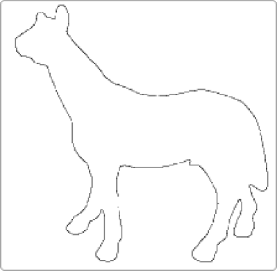
Figure 9: $\quad P(\mbox{1 hole})\approx 52.7\%$, $\quad P(\mbox{2 holes})\approx 25.8\%$, $P(\mbox{3 holes})\approx 9.4\%$, $\;P(\mbox{4 holes})\approx 2\%$, $\;P(\mbox{5 holes})\approx 0.5\%$.

The left hand side pictures in Fig. 10–14 are from http://www.lems.brown.edu/~dmc. The right hand side pictures are extracted contours with added noise.

Figure 10: $\quad P(\mbox{1 hole})\approx 88.4\%$, $\quad P(\mbox{2 holes})\approx 1.5\%$, $P(\mbox{0 holes})\approx 0.9\%$, $\;P(\mbox{13 holes})\approx 0.5\%$, $\;P(\mbox{5 holes})\approx 0.4\%$.

Figure 11: $\quad P(\mbox{1 hole})\approx 66\%$, $\quad P(\mbox{2 holes})\approx 11\%$, $P(\mbox{3 holes})\approx 3.8\%$, $\;P(\mbox{4 holes})\approx 3.3\%$, $\;P(\mbox{6 holes})\approx 1.1\%$.

Figure 12: $\quad P(\mbox{1 hole})\approx 58.3\%$, $\quad P(\mbox{2 holes})\approx 19.3\%$, $P(\mbox{3 holes})\approx 4.2\%$, $\;P(\mbox{4 holes})\approx 1.6\%$, $\;P(\mbox{8 holes})\approx 0.8\%$.

Figure 13: $\quad P(\mbox{1 hole})\approx 49.6\%$, $\quad P(\mbox{2 holes})\approx 21.1\%$, $P(\mbox{3 holes})\approx 4.7\%$, $\;P(\mbox{4 holes})\approx 3.3\%$, $\;P(\mbox{5 holes})\approx 1.8\%$.

Figure 14: $\quad P(\mbox{2 holes})\approx 43.7\%$, $\quad P(\mbox{1 hole})\approx 27.8\%$, $P(\mbox{3 holes})\approx 2.5\%$, $\;P(\mbox{5 holes})\approx 2.1\%$, $\;P(\mbox{6 holes})\approx 1.6\%$.

The left hand side pictures in Fig. 15–17 contain a cloud $C$ uniformly generated around wheels (the boundaries of regular polygons with the radii to all vertices). The middle pictures show the persistence diagrams $\mathrm{PD}\{C^{\alpha}\}$. The right hand side pictures are the staircases $\mathrm{PS}\{C^{\alpha}\}$ giving the number of holes of $C$ depending on the scale $\alpha$.

The left hand side pictures in Fig. 18–20 are noisy clouds around square lattices containing $25,36,49$ small squares. The algorithm HoCToP finds the expected number $49$ of holes in Fig. 20 when even humans may struggle.

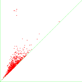
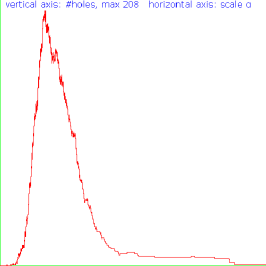
Figure 15: $\quad P(\mbox{7 holes})\approx 22\%$, $\quad P(\mbox{1 hole})\approx 14\%$, $\quad P(\mbox{8 holes})\approx 7.5\%$, $\quad P(\mbox{6 holes})\approx 5.8\%$, $\quad P(\mbox{10 holes})\approx 4.4\%$.

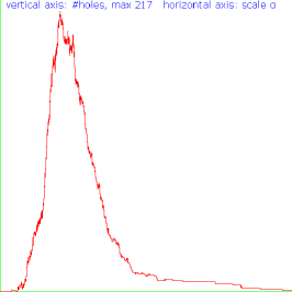
Figure 16: $\quad P(\mbox{8 holes})\approx 11.5\%$, $\quad P(\mbox{2 holes})\approx 8.5\%$, $\quad P(\mbox{3 holes})\approx 7\%$, $\quad P(\mbox{9 holes})\approx 6.8\%$, $\quad P(\mbox{6 holes})\approx 6.5\%$.

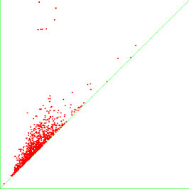
Figure 17: $\quad P(\mbox{9 holes})\approx 18.5\%$, $\quad P(\mbox{10 holes})\approx 11.3\%$, $\quad P(\mbox{3 holes})\approx 6.8\%$, $\quad P(\mbox{3 holes})\approx 6.8\%$, $\quad P(\mbox{4 holes})\approx 5.3\%$.

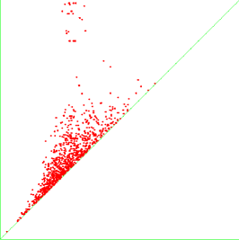
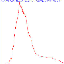
Figure 18: $\quad P(\mbox{25 holes})\approx 8.8\%$, $\quad P(\mbox{0 holes})\approx 5.4\%$, $\quad P(\mbox{15 holes})\approx 5\%$, $\quad P(\mbox{27 holes})\approx 4.6\%$, $\quad P(\mbox{20 holes})\approx 3.5\%$.

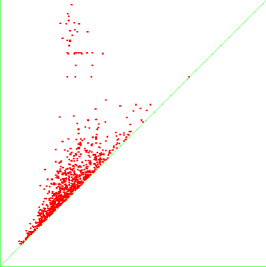
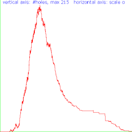
Figure 19: $\quad P(\mbox{36 holes})\approx 9.4\%$, $\quad P(\mbox{31 holes})\approx 4.8\%$, $\quad P(\mbox{33 holes})\approx 4.8\%$, $\quad P(\mbox{2 holes})\approx 4.6\%$, $\quad P(\mbox{1 hole})\approx 3.2\%$.

Figure 20: $\quad P(\mbox{49 holes})\approx 18.4\%$, $\quad P(\mbox{52 holes})\approx 4.9\%$, $\quad P(\mbox{1 hole})\approx 3.3\%$, $\quad P(\mbox{6 holes})\approx 2.8\%$, $\quad P(\mbox{0 holes})\approx 2.7\%$.

References

- [1] D. Attali, M. Glisse, S. Hornus, F. Lazarus, and D. Morozov. Persistence-sensistive simplification of functions on surfaces in linear time. TopoInVis 2009.
- [2] M. de Berg, O. Cheong, M. van Kreveld, and M. Overmars. Computational Geometry: Algorithms and Applications. Springer, 2008.
- [3] F. Chazal, L. Guibas, S. Oudot, P. Skraba. Scalar Field Analysis over Point Cloud Data. Discrete and Computational Geometry, v. 46 (2011), p.743-775.
- [4] D. Cohen-Steiner, H. Edelsbrunner, and J. Harer. Stability of persistence diagrams. Discrete and Computational Geometry, 37:103–130, 2007.
- [5] H. Edelsbrunner. The union of balls and its dual shape. Discrete Computational Geometry, 13:415–440, 1995.
- [6] H. Edelsbrunner and J. Harer. Computational topology. An introduction. AMS, Providence, 2010.
- [7] Letscher, D., Fritts, J. Image segmentation using topological persistence. Proceedings of CAIP 2007: Computer Analysis of Images and Patterns, pages 587–595.
- [8] N. Milosavljevic, D. Morozov, and P. Skraba. Zigzag persistent homology in matrix multiplication time. Proceedings of SoCG 2011, pages 216–225, ACM.