Electron-electron interactions in bilayer graphene quantum dots

Abstract

A parabolic quantum dot (QD) as realized by biasing nanostructured gates on bilayer graphene is investigated in the presence of electron-electron interaction. The energy spectrum and the phase diagram reveal unexpected transitions as function of a magnetic field. For example, in contrast to semiconductor QDs, we find a novel valley transition rather than only the usual singlet-triplet transition in the ground state of the interacting system. The origin of these new features can be traced to the valley degree of freedom in bilayer graphene. These transitions have important consequences for cyclotron resonance experiments.

I Introduction

The electronic properties of quantum dots (QDs) in graphene, a single layer of carbon atoms arranged in a honeycomb lattice geim ; tapash_review ; sarma have been studied extensively due to their unique properties and their potential for applications in graphene devices ensslin ; nori ; hawrylak ; matulis . Since Klein tunneling prevents electrostatic confinement in graphene, direct etching of the graphene sheet is perhaps the only viable option for quantum confinement. In such systems, controlling the shape and edges of the dot remains an important challenge but the exact configuration of the edges is unknown ritter . The latter is important because the energy spectrum depends strongly on the type of edges marko ; zarenia1 .

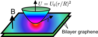
Figure 1: (Color online) Schematic illustration of the potential profile for a parabolic bilayer graphene quantum dot.

Two coupled layers of graphene, called bilayer graphene (BLG), have quite distinct properties from those of a single layer. In pristine BLG the spectrum is gapless and is approximately parabolic at low energies around the two nonequivalent points in the Brillouin zone ($K$ and $K^{\prime}$). In a perpendicular electric field, the spectrum displays a gap which can be tuned by varying the bias zhang . Nanostructuring the gate would allow tuning of the energy gap in BLG which can be used to electrostatically confine QDs milton1 ; milton2 and quantum rings zarenia . Here the electrons are displaced from the edge of the sample and consequently edge disorder and the specific type of edges are no longer a problem. Such gate defined QDs in BLG were recently fabricated by different groups allen ; QD2 ; muller , who demonstrated experimentally the confinement of electrons and Coulomb blockade.

In the present work we investigate the energy levels of a parabolic QD in BLG in the presence of Coulomb interaction. Here we consider the two-electron problem as the most simple case to investigate the effect of electron-electron correlations. Similar studies have been reported for semiconducting QDs over the last two decades wagner ; tapash and recently for graphene QDs wunsch and graphene rings abergel . At present no similar study has been reported for BLG quantum dots. An important issue for graphene structures is the extra valley-index degree of freedom where the electrons have the possibility to be in the same valley or in different valleys review ; sabio . Here we show that the competition between the valley-index and the electron spin leads to unique behaviors that shed light on the fundamental properties of the ground state energy of BLG quantum dots.

II Continuum model

In order to find the single-particle energy spectrum of a parabolic QD we employ a four-band continuum model to describe the BLG sheet. In the valley-isotropic form Falko , the Hamiltonian is given by

$$H=\begin{pmatrix}\tau U(r)&\pi&t&0\\ \pi^{\dagger}&\tau U(r)&0&0\\ t&0&-\tau U(r)&\pi^{\dagger}\\ 0&0&\pi&-\tau U(r)\end{pmatrix}$$ (1)

where $t\approx 400$ meV is the inter-layer coupling term. The additional coupling terms which lead to the trigonal warping effect are neglected. The trigonal warping effect is only relevant at very low energies (i.e. $E<2$ meV) in the absence of an electrostatic potential Falko . $\pi=-i\hbar v_{F}e^{i\theta}\big{[}\partial_{r}+i\partial_{\theta}/r-(eB/2\hbar)r\big{]}$ is the momentum operator in polar coordinates and in the presence of an external magnetic field $B$, and $v_{F}=10^{6}$ m/s is the Fermi velocity. The valley index parameter $\tau$ distinguishes the energy levels corresponding to the $K$ ($\tau=+1$) and the $K^{\prime}$ ($\tau=-1$) valleys. The electrostatic potential $U(r)$ is applied to the upper layer and $-U(r)$ to the lower layer. For the QD profile we consider a parabolic potential $U(r)=U_{b}(r/R)^{2}$ where the potential $U_{b}$ and the radius $R$ define the size of the dot [Fig. 1]. The eigenstates of the Hamiltonian (1) are the four-component spinors

$$\psi(r,\theta)=e^{im\theta}\big{[}\phi_{A}(r),e^{-i\theta}\phi_{B}(r),\phi_{B^{\prime}}(r),e^{i\theta}\phi_{A^{\prime}}(r)\big{]}^{T}$$ (2)

where $\phi_{A,B,B^{\prime},A^{\prime}}$ are the envelope functions associated with the probability amplitudes at the respective sublattice sites of the upper and lower graphene sheets and $m$ is the angular momentum. The orbital angular momentum $L_{z}$ does not commute with the Hamiltonian and is no longer quantized. This is different from two-dimensional semiconductor QDs, where $[H,L_{z}]=0$. However, the wave function $\psi(r,\phi)$ is an eigenstate of the operator

$$J_{z}=L_{z}+\left[\frac{\hbar}{2}\left(\begin{array}[]{cc}-\boldsymbol{I}&0\\ 0&\boldsymbol{I}\\ \end{array}\right)+\frac{\hbar}{2}\left(\begin{array}[]{cc}\sigma_{z}&0\\ 0&-\sigma_{z}\\ \end{array}\right)\right]$$ (3)

with eigenvalue $m$, where $\boldsymbol{I}$ is the $2\times 2$ unitary matrix and $\sigma_{z}$ is one of the Pauli matrices. The first operator inside the bracket is a layer index operator, which is associated with the behavior of the system under inversion, whereas the second one denotes the pseudospin components in each layer.

Solving the Shrödinger equation, $H\Psi=E\Psi$, the radial dependence of the spinor components is described by

$$\Bigl{[}\frac{d}{dr}+\frac{m}{r}+\beta r\Bigr{]}\phi_{A}=-\big{[}E-\tau U(r)\big{]}\phi_{B},$$ (4)

(5)

$$\Bigl{[}\frac{d}{dr}-\frac{(m-1)}{r}-\beta r\Bigr{]}\phi_{B}=\big{[}E-\tau U(r)\big{]}\phi_{A}-t\phi_{B^{\prime}},$$ (6)

(7)

$$\Bigl{[}\frac{d}{dr}+\frac{(m+1)}{r}+\beta r\Bigr{]}\phi_{A^{\prime}}=\big{[}E+\tau U(r)\big{]}\phi_{B^{\prime}}-t\phi_{A},$$ (8)

(9)

$$\Bigl{[}\frac{d}{dr}-\frac{m}{r}-\beta r\Bigr{]}\phi_{B^{\prime}}=-\big{[}E+\tau U(r)\big{]}\phi_{A^{\prime}}$$ (10)

where $\beta=(eB/2\hbar)R^{2}$ is a dimensionless parameter. The energy, the potential and the hopping term $t$ are written in units of $E_{0}=\hbar v_{F}/R$ with $R$ being the unit of length. The coupled equations (4) are solved numerically using the finite element method comsol .

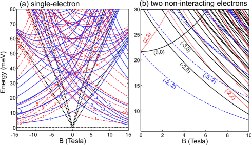
Figure 2: (Color online) Energy spectrum of a parabolic QD in BLG with $R=50$ nm and $U_{b}=150$ meV as a function of the magnetic field for (a) single-particle and (b) two noninteracting electrons. The lowest energy levels in (a) are labeled by the angular momentum $m$. The levels corresponding to the $K$ and $K^{\prime}$ valleys are respectively shown by the blue solid and red dashed curves. The black dotted curves are the Landau levels of a BLG sheet. The levels in (b) are labeled by $(M,{\cal T})$, where $M=m_{1}+m_{2}$, is the total angular momentum and ${\cal T}=\tau_{1}+\tau_{2}$ is the total valley index. Levels having the same valley index are plotted using the same type of curve.

II.1 Single-particle energy levels

Figure 2(a) shows the lowest single-electron energy levels as a function of the magnetic field for a QD with $U_{b}=150$ meV and $R=50$ nm. The energy levels are labeled by their angular momentum and their valley index ($m,\tau$). We begin with the $B=0$ case. Notice that the single-particle ground state does not have $m=0$ as expected for semiconductor QDs, but instead has the momentum $m=1$ at $K$ and $m=-1$ at $K^{\prime}$ in agreement with Ref. milton1 .

For large magnetic fields the eigenstates are strongly localized at the origin of the dot, where $\Delta U\rightarrow 0$. Therefore, the spectrum approaches the Landau levels (LLs) of an unbiased BLG (black dotted curves in Fig. 2(a)) and consequently some of the energy levels approach $E=0$ as the field increases. Notice that this is quite distinct from semiconductor QDs where the zeroth LL is absent and thus the energy of the confined stats, i.e., the Fock-Darwin states, increase with magnetic field. Breaking of the electron-hole symmetry due to the presence of both electric and magnetic fields lifts the valley-degeneracy in non-zero magnetic fields. The energy spectrum also displays the $E_{K}(m,B)=E_{K^{\prime}}(-m,-B)$ symmetry, which is another feature that is unique to BLG quantum dots. This symmetry is a consequence of the fact that the QD is produced by a gate that introduces an electric field and thus a preferential direction. Inserting $(m,\beta)\rightarrow(-m,-\beta)$ and $\tau\rightarrow-\tau$ in Eqs. (4) and using $E_{\tau}(m,B)=E_{-\tau}(-m,-B)$, one can find the relations $\phi_{A}^{K}(m,B)=\phi_{B^{\prime}}^{K^{\prime}}(-m,-B)$ and $\phi_{B}^{K}(m,B)=\phi_{A^{\prime}}^{K^{\prime}}(-m,-B)$ between the wave function components of the $K$ and $K^{\prime}$ valleys.

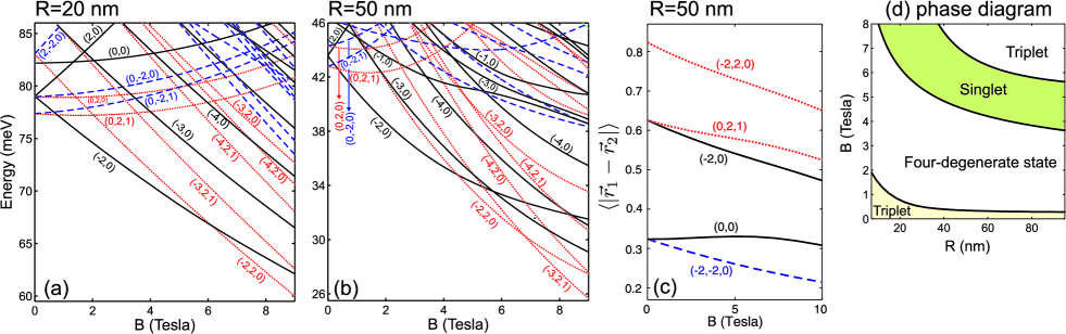
Figure 3: (Color online) (a,b) The same as Fig. 2(b) but in the presence of Coulomb interaction and for (a) $R=20$ nm and (b) $R=50$ nm. The levels are labeled by $(M,{\cal T},S)$ where $S$ indicates the total spin. The curves with the same total valley index ${\cal T}$ are shown with the same type of curve. (c) The average distance between the electrons as function of magnetic field for different single particle basis functions. (d) The radius-magnetic field ($R-B$) phase diagram of the ground state energy of a two-electron BLG quantum dot.

II.2 Two-electron energy spectrum

The Hamiltonian describing the two-electron system is given by $H_{T}=H({\bf r}_{1})+H({\bf r}_{2})+V_{c}({\bf r}_{1}-{\bf r}_{2})$ where $V_{c}=e^{2}/(4\pi\kappa|{\bf r}_{1}-{\bf r}_{2}|)$ is the Coulomb interaction between the two electrons with $\kappa$ being the dielectric constant of BLG. In our calculations we set $\kappa=3.9$ which is the dielectric constant of gated BLG on top of a hexagonal boron nitride (h-BN) substrate Dean . We carry out an exact diagonalization of the above Hamiltonian to obtain the eigenvalues and eigenstates of the two-electron system. The corresponding two-electron wave function with fixed total angular momentum $M$ and total valley index ${\cal T}$ is constructed as linear combinations of the one-electron wave functions:

$$\Psi({\bf r}_{1},{\bf r}_{2})=\sum_{i}^{N_{s}}\sum_{j}^{N_{s}}C_{ij}\Phi_{i}({\bf r}_{1})\otimes\Phi_{j}({\bf r}_{2})$$ (11)

where $\Phi$ is a eight-component wave function which is $\Phi_{K}=[~{}\psi_{K},~{}0,~{}0,~{}0,~{}0~{}]^{T}$ corresponding to the $K$ valley and $\Phi_{K^{\prime}}=[~{}0,~{}0,~{}0,~{}0,~{}\psi_{K^{\prime}}~{}]^{T}$ corresponding to the $K^{\prime}$ valley bloch . The four-component wave function $\psi_{K(K^{\prime})}$ is given by Eq. (2). Notice that the two-electron wave function $\Psi({\bf r}_{1},{\bf r}_{2})$ has sixty-four components. The subscripts $i\equiv(m_{i},\tau_{i})$ and $j\equiv(m_{j},\tau_{j})$ correspond to the one-electron energy levels where the summations in Eq. (11) are such that the relations $M=m_{i}+m_{j}$ and ${\cal T}=\tau_{i}+\tau_{j}$ are satisfied. In our calculations $N_{s}$, i.e. the number of lowest single-particle states, is chosen sufficiently large to guarantee the convergence of the energies. The singularity due to the $1/|{\bf r}_{1}-{\bf r}_{2}|$ term in the matrix elements is avoided by using an alternative expression in terms of the Legendre function of the second kind of half-integer degree cohl .

In Fig. 3, we show two representative spectra for two interacting electrons in a BLG quantum dot with radius (a) $R=20$ nm, and (b) $R=50$ nm, and $U_{b}=150$ meV. To clearly see the effect of electron correlations, the spectra for two non-interacting electrons in a dot with $R=50$ nm is shown in Fig. 2(b) for comparison. The levels are labeled by $(M,{\cal T},S)$ with $M=m_{1}+m_{2}$ the total angular momentum, ${\cal T}=\tau_{1}+\tau_{2}$ the total valley index, and $S$ the total spin. Energy levels with the same $\cal T$ are drawn using the same type of curve. Two electrons can form a non-degenerate singlet state ($S=0$) and a three-fold degenerate triplet state ($S=1$). In case the quantum number $S$ is omitted, the singlet and triplet states are degenerate. In the following discussion it is useful to characterize the many-body state by the single particle basis function in expression (11) which has the largest contribution. We denote the basis function in which the first and second electron have, respectively, angular momentum $m_{1}$ and $m_{2}$ and valley index $\tau_{1}$ and $\tau_{2}$ as $(m_{1},\tau_{1})\otimes(m_{2},\tau_{2})\equiv\phi_{m_{1},\tau_{1}}\otimes\phi_{m_{2},\tau_{2}}$.

The spectra of the two interacting electrons in Figs. 3(a) and 3(b) are a result of three competing effects. It is evident that the energy of the single particle states as function of the magnetic field, shown in Fig. 2(b), determines partly the spectrum. However, turning on the Coulomb interaction between the electrons changes the spectrum drastically. While the non-interacting state $(-2,-2)\equiv(-1,-1)\otimes(-1,-1)$ is the ground state, the many-body interacting state in which this single particle basis function has the largest contribution is an excited state and does not even appear in Figs. 3(a) and 3(b). Instead the many-body state $(0,2,1)$ is the ground state for small magnetic field values, with the main contribution $(1,1)\otimes(-1,1)$. The Coulomb interaction is clearly not a small perturbation. In Fig. 3(c), the evolution of the average distance between both electrons is shown for different single particle basis states (for the $R=50$ nm case). This difference in the average distance can be understood from the single particle densities. While single particle states $(-1,-1)$ and $(1,1)$ have a non-zero density in the origin, the density of the single particle state $(-1,1)$ is zero in the origin. Therefore, this average distance is much larger, and consequently the Coulomb interaction is much lower, for the basis function $(1,1)\otimes(-1,1)$ than for $(-1,-1)\otimes(-1,-1)$, which is the reason why the many-body state $(0,2,1)$ has a lower energy.

A more subtle effect is played by the exchange interaction. As mentioned, the ground state at small magnetic field values is given by the many-body state $(0,2,1)$, which is a triplet state. The corresponding singlet state $(0,2,0)$ is slightly higher in energy. Also note that the state $(-2,0)$, with the main single particle contribution $(-1,1)\otimes(-1,-1)$ is higher in energy at small magnetic fields, although the Coulomb interaction contribution is expected to be very similar (compare curves $(0,2,1)$ and $(-2,0)$ in Fig. 3(c)). The reason is again the exchange interaction energy gain for the triplet state $(0,2,1)$. State $(-2,0)$ is fourfold degenerate: the triplet configuration does not lead to an exchange energy gain because both electrons occupy different valleys. Only for larger magnetic field values, the state $(-2,0)$ takes over from the state $(0,2,1)$ to become the ground state. This is caused by the evolution of the single particle energies. The next state that becomes the ground state with increasing magnetic field is the singlet $(-2,2,0)$, with main single particle contribution $(-1,1)\otimes(-1,1)$. Because twice the same single particle level is occupied, no exchange energy gain is possible. Nevertheless, this state becomes the ground state due to the evolution of the single particle energies, together with the fact that the average distance between both electrons is even smaller (see Fig. 3(c)), as both electrons occupy a single particle level with zero density in the origin. With increasing field, it becomes beneficial for an electron to jump from the single particle level $(-1,1)$ to the single particle level $(-2,1)$, resulting in the triplet state $(-3,2,1)$ with main contribution $(-2,1)\otimes(-1,1)$.

While in conventional semiconductor QDs, the ground state shows a series of singlet to triplet transitions as function of the magnetic field strength tapash ; wagner , a more complex phase diagram is found for BLG QDs. In Fig. 3(d) we plot this phase diagram for the same $U_{b}$ and dielectric constant as used for Fig. 3(a,b). For small magnetic field values, the ground state is found to be a triplet state. With increasing field a valley transition occurs, resulting in a fourfold-degenerate state. Next, again a valley transition occurs into a singlet state. Further increasing the magnetic field favors again a triplet state.

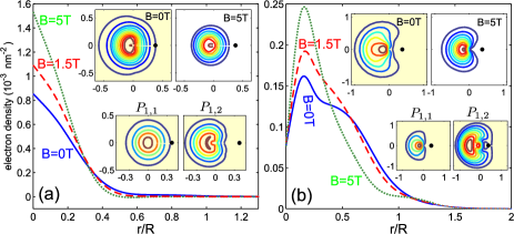
Figure 4: (Color online) The radial electron density for the two-electron QD of Fig. 3(b) for (a) $(M,{\cal T})\equiv(-2,0)$ and (b) $(M,{\cal T},S)\equiv(-3,2,1)$ and for $B=0$, $1.5$, $5$ T. The upper insets show the total pair-correlation function for $B=0$ T and $B=5$ T. The lower insets show separate parts of the pair-correlation function for $B=0$. The black dot indicates the position of the first electron which is pinned at ${\bf r}_{1}=(0.4R,0)$.

The electron density, $\rho(r)=\sum_{i=1}^{2}\langle\delta({\bf r}-{\bf r}_{i})\rangle$ is shown in Figs. 4(a) and 4(b), respectively for the $(-2,0)$ and $(-3,2,1)$ states, of a two-electron BLG quantum dot with $R=50$ nm, $U_{b}=150$ meV, and for three values of the external magnetic field $B=0,1.5,5$ T. Comparing the density profiles in (a) and (b), the maximum of the density is shifted towards higher radial distance in the state $(-3,2,1)$. This is a consequence of the fact that the electrons in the many-particle $(-3,2,1)$ state occupy single-particle states with higher angular momentum. As the magnetic field increases, the electrons are pulled closer towards the center of the dot. The upper insets in Figs. 4(a) and 4(b) show the total pair-correlation function $P=|\Psi({\bf r},{\bf r}_{2})|^{2}=P_{1,1}+P_{1,2}$, for $B=0$ T and $B=5$ T. The $P_{1,1}$, and $P_{1,2}$ terms refer respectively to the contribution of the sublattices in the same layer and in the different layers. In the lower insets the terms $P_{1,1}$ and $P_{1,2}$ are plotted separately for $B=0$ T which respectively indicate the probability to find the second electron in the same layer, or in the other layer if the first electron is fixed at a certain point.

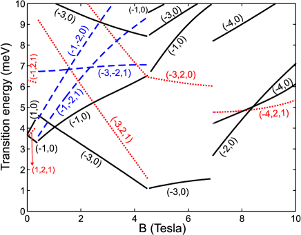
Figure 5: (Color online) The cyclotron transition energies for the QD of Fig. 3(b). The transition energies are labeled by their final states: $(M,{\cal T},S)$ for the triplet (or singlet) states and $(M,{\cal T})$ for the degenerate single-triplet states. Levels having the same total valley index are plotted using the same type of curve.

In cyclotron resonance experiments, transitions are induced between the ground state and excited states. For the BLG quantum dot the selection rule on the change of total momentum $\Delta m=\pm 1$ is still fulfilled. This is apparent when we calculate the transition energies and the corresponding transition rates for dipole transitions using the relation $|\langle\Psi_{i}|\sum_{j=1}^{2}r_{j}\exp{(\pm i\theta_{j})}/2|\Psi_{f}\rangle|^{2}$. This relation also implies conservation of the total spin, i.e., $\Delta S=0$. The valley degree of freedom dictates new transition rules for BLG quantum dots, i.e., $\Delta{\cal T}=0$ or $\Delta{\cal T}=\pm 2$. This means that those transitions are possible in which at least one electron remains in the same valley during the transition. The lowest possible transition energies for a two-electron quantum dot with $R=50$ nm and $U_{b}=150$ meV are shown in Fig. 5. The possible transitions are labeled by the final states ($M,{\cal T},S$). The discontinuities between the transition energies at $B\approx 0.5$ T, $B\approx 0.5$ T and $B\approx 7$ T are due to the valley and singlet-triplet transitions (see Fig. 3(b)).

III CONCLUDING REMARKS

In summary, we have investigated the energy levels, the electron density, the pair correlation function and the cyclotron transition energies of electrostatically confined QDs containing one or two electrons in a BLG. Such QDs can be realized experimentally by using nanostructured gate potentials on a BLG. In contrast to conventional semiconductor QDs, we found that the ground state energy of the two-electron spectrum exhibits a valley transition rather than a spin singlet-triplet transition. This is due to the extra valley degree of freedom in BLG in which the electrons can be in different valleys and thereby allowing the four-degenerate single-triplet states as the ground state. Experimental confirmation of our prediction can come from spin susceptibility measurements.

References

- (1) A.H. Castro Neto, F. Guinea, N.M.R. Peres, K.S. Novoselov, and A.K. Geim, Rev. Mod. Phys. 81, 109 (2009).
- (2) D.S.L. Abergel, V. Apalkov, J. Berashevich, K. Ziegler, and T. Chakraborty, Adv. Phys. 59, 261 (2010).
- (3) S. Das Sarma, Sh. Adam, E.H. Hwang, and E. Rossi, Rev. Mod. Phys. 83, 407 (2011).
- (4) J. Güttinger, F. Molitor, C. Stampfer, S. Schnez, A. Jacobsen, S. Dröscher, T. Ihn, and K. Ensslin, Rep. Prog. Phys. 75, 126502 (2012).
- (5) A.V. Rozhkov, G. Giavaras, Y.P. Bliokh, V. Freilikher, and F. Nori, Phys. Rep. 503, 77 (2011).
- (6) Wei-dong Sheng, M. Korkusinski, A.D. Güclü, M. Zielinski, P. Potasz, E.S. Kadantsev, O. Voznyy, and P. Hawrylak, Front. Phys. 7, 328 (2012).
- (7) A. Matulis and F.M. Peeters, Phys. Rev. B 77, 115423 (2008).
- (8) K.A. Ritter and J.W. Lyding, Nature Materials 8, 235 (2009).
- (9) M. Grujić, M. Zarenia, A. Chaves, M. Tadić, G.A. Farias, and F.M. Peeters, Phys. Rev. B 84, 205441 (2011); S. Schnez, K. Ensslin, M. Sigrist, and T. Ihn, ibid. 78, 195427 (2008).
- (10) M. Zarenia, A. Chaves, G.A. Farias, and F.M. Peeters, Phys. Rev. B 84, 245403 (2011).
- (11) Y. Zhang, Tsung-Ta Tang, C. Girit, Zhao Hao, M.C. Martin, A. Zettl, M.F. Crommie, Y. Ron Shen, and F. Wang, Nature (London) 459, 820 (2009).
- (12) J.M. Pereira Jr., P. Vasilopoulos, and F.M. Peeters, Nano Lett. 7, 946 (2007).
- (13) J.M. Pereira Jr., F.M. Peeters, P. Vasilopoulos, R.N. Costa Filho, and G.A. Farias, Phys. Rev. B 79, 195403 (2009).
- (14) M. Zarenia, J.M. Pereira, Jr., F.M. Peeters, and G.A. Farias, Nano Lett. 9, 4088 (2009).
- (15) M.T. Allen, J. Martin, and A. Yacoby, Nature Comm. 3, 934 (2012).
- (16) A.M. Goossens, S.C.M. Driessen, T.A. Baart, K. Watanabe, T. Taniguchi, and L.M.K. Vandersypen, Nano Lett. 12, 4656 (2012).
- (17) A. Müller, B. Kaestner, F. Hohls, Th. Weimann, K. Pierz, and H.W. Schumacher, arXiv:1304.7661.
- (18) M. Wagner, U. Merkt and A.V. Chaplik, Phys. Rev. B 45, 1951 (1992).
- (19) P.A. Maksym and T. Chakraborty, Phys. Rev. Lett. 65, 108 (1990); F.M. Peeters and V.A. Schweigert, Phys. Rev. B 53, 1468 (1996).
- (20) B. Wunsch, T. Stauber, and F. Guinea, Phys. Rev. B 77, 035316 (2008).
- (21) D.S.L. Abergel, V.M. Apalkov, and T. Chakraborty, Phys. Rev. B 78, 193405 (2008).
- (22) V.N. Kotov, B. Uchoa, V.M. Pereira, F. Guinea, and A.H. Castro Neto, Rev. Mod. Phys. 84, 1067 (2012).
- (23) J. Sabio, F. Sols, and F. Guinea, Phys. Rev. B 81, 045428 (2010).
- (24) E. McCann and V. I. Fal´ko, Phys. Rev. Lett. 96, 086805 (2006).
- (25) In order to solve the system of Eqs. (4) numerically we used the COMSOL package: www.comsol.com
- (26) C.R. Dean, A.F. Young, I. Meric, C. Lee, L. Wang, S. Sorgenfrei, K. Watanabe, T. Taniguchi, P. Kim, K.L. Shepard, and J. Hone, Nature Nanotechnology 5, 722 (2010).
- (27) The total single particle wave functions can be expressed as a superposition of the contribution of the two valleys via the Bloch wave function, i.e. and . When both electrons are in the same valley the Bloch terms cancel each other and when the electrons belong to different valleys the corresponding matrix element becomes zero . Thus the Bloch wave functions are not important when constructing the matrix elements.
- (28) H.S. Cohl, A.R.P. Rau, Joel E. Tohline, D.A. Browne, J.E. Cazes, and E.I. Barnes, Phys. Rev. A 64, 052509 (2001).