The initial condition problems of damped quantum harmonic oscillator

Abstract

We investigate the exact dynamics of the damped quantum harmonic oscillator under the (un)correlated initial conditions. The master equation is generalized to the cases of the arbitrary factorized state and/or Gaussian state. We show that the variances of the factorized Gaussian state do not sensitively depend on the initial oscillator-bath correlation, which however can remarkably affect the mean values even at high temperature. We also illustrate that the correlations among the factorized states still give rise to the initial dips during the purity evolutions, which can be smoothed out by increasing the amount of correlation to some extent. We finally study the effects of repeated measurements on the time evolution of the damped oscillator analytically, which are compared with the weak coupling results to indicate that they give rather different transient behaviors even for an intermediate coupling.

I Introduction

The recent experimental developments in the field of ultrafast and ultrasmall devices at low temperature are strongly demanding for the fully treatments of the non-Markovian dynamics of open quantum systems open , which go beyond the traditional Markovian approximation omitting the memory effects of surrounding bath in the weak coupling limit. The rigorous analysis has been explored extensively in the literature. For example, the exact master equation of quantum Brownian motion was derived by the path integral phpz ; hpz ; kg , which has been extended to other open systems ext , such as quantum dots, the nano-cavities, and quantum transportation in photonic crystals. On the other hand, in most of these studies, the initial system-bath correlations are often neglected for mathematical simplicity, the roles of which in realistic could become significant for the strongly coupled system-bath interactions. It is shown that the initial qubit-bath correlations can break the completely positive property of the evolution maps–leading to nontrivial differences in quantum tomography process qt , and can be witnessed by the increase of the distance of two system states over its initial value measure . Besides, it is found that the effects of the initial correlations on the photon squeezing in a cavity, the coherence of a qubit, the entanglement of two-qubit, and etc, can induce the oscillating dynamics in the strong non-Markovian regime initial .

In this paper, we continue to investigate the exact dynamics in the presence of the initial correlations with the dissipative quantum harmonic oscillator as an example. The initial oscillator-bath correlations are incorporated in two different ways: (i) prepare an initial state by implementing some measurements on an prior state, such as a projective measurement acting only on the oscillator, which does not change its equation of motion dist ; (ii) alter the equation of motion of the oscillator by adjusting its parameters–mass or frequency at an initial time, whereas the initial state is untouched cl . From the general solutions to quantum Langevin equation (QLE), the time evolutions of oscillator are simply derived by using the Wigner representations of operators and the Gaussian properties of the total system, which allow us to examine the existence of the master equation for the oscillator and specify the conditions resulting in some certain master equations straightforwardly. We also get a time-local QLE by introducing an effective fluctuation force, and apply the modified canonical method used by Unruh and Zurek in uz to derive the exact master equations for the factorized initial conditions, which can in further include the cases of initial correlated Gaussian states.

We show that for the factorized Gaussian state, the initial oscillator-bath correlation plays unimportant roles for the variances over a wide range (except the regime of under-damping) of coupling strength. However, the effect of initial correlation becomes remarkable for the expectation values even at high temperature. We illustrate that the initial correlations in the factorized states are not enough to smooth out the initial dips displayed during the purity evolutions. By increasing the amount of initial correlations to some extent, these dips just disappear. We also study the effects of repeated measurements on the time evolution of the damped oscillator analytically. The comparison with the weak coupling results is made to indicate that even for an intermediate coupling, they have rather different transient behaviors.

The rest of this paper is as follows. In Sec. II, we briefly review the basics of QLE for subsequent discussions. The exact dynamics with the initial correlations is obtained through the Wigner representation in Sec. III. Next, in Sec. IV we use the canonical method to derive the master equations for the factorized initial conditions. Then in Sec. V we give some examples to show the implications of the previous results. Finally, a short summary is given in Sec. VI.

II The equations of motion

The interacting oscillator-bath Hamiltonian to model the damped harmonic oscillator is usually taken as qle ,

$$H={p^{2}\over 2m}+{1\over 2}kx^{2}+\sum_{j}\left[{p_{j}^{2}\over 2m_{j}}+{1\over 2}m_{j}\omega_{j}^{2}(q_{j}-x)^{2}\right].$$ (1)

In the Heisenberg picture with the natural units $\hbar=k_{B}=m=1$, the equations of motion of the oscillator take the form of an initial value problem,

$$\ddot{x}(t)+\int_{0}^{t}dt^{\prime}\mu(t-t^{\prime})\dot{x}(t^{\prime})+kx(t) = -\mu(t)x(0)+F(t),$$

$$\dot{x}(t) = p(t),$$ (2)

which are known as the QLE for dissipative harmonic oscillator. Here the memory kernel and fluctuating force are

$$\mu(t)=\sum_{j}m_{j}\omega_{j}^{2}\cos(\omega_{j}t),\quad t>0,\hskip 28.45274pt$$ (3)

$$F(t)=\sum_{j}m_{j}\omega_{j}^{2}\left[q_{j}(0)\cos(\omega_{j}t)+p_{j}(0)\frac{\sin(\omega_{j}t)}{m_{j}\omega_{j}}\right].$$ (4)

The two quantities are connected through the commutator, $[F(t),F(0)]=i\dot{\mu}(t)$, which is necessary for the conservation of the elementary commute relation $[x(t),p(t)]=i$ for $t\geq 0$. It can be seen that $[x(0),F(t)]=0$ and $[\dot{x}(0),F(t)]=0$ because $F(t)$ only depends on the bath variables at $t=0$. The general solution of (2) yields to be

$$x(t) = \dot{G}(t)x(0)+G(t)p(0)+X(t),$$ (5)

$$p(t) = \ddot{G}(t)x(0)+\dot{G}(t)p(0)+\dot{X}(t),$$ (6)

where

$$X(t)=\int_{0}^{t}dt^{\prime}G(t-t^{\prime})F(t^{\prime}),$$ (7)

and the retarded Green function $G(t)$ for $t>0$ satisfies the equation

$$\ddot{G}(t)+\int_{0}^{t}dt^{\prime}\mu(t-t^{\prime})\dot{G}(t^{\prime})+kG(t)=0.$$ (8)

and $G(t)=0$ when $t<0$. At $t=0$, the conditions $G(0)=0$ and $\dot{G}(0)=1$ are imposed. In the following we set $t\geq 0$ for convenience. Explicitly, $G(t)$ can be expressed by the Fourier integral,

$$G(t) = {1\over 2\pi}\int_{-\infty}^{\infty}d\omega\alpha(\omega)e^{-i\omega t}$$ (9)

$$= {2\over\pi}\int_{0}^{\infty}d\omega\alpha^{\prime\prime}(\omega)\sin(\omega t),$$

where the susceptibility $\alpha(\omega)=\alpha^{\prime}(\omega)+i\alpha^{\prime\prime}(\omega)$ is

$$\alpha(\omega)=\frac{1}{-\omega^{2}-i\omega\eta(\omega)+k}.$$ (10)

Here

$$\eta(\omega)=\eta^{\prime}(\omega)+i\eta^{\prime\prime}(\omega)=\int_{0}^{\infty}dt\mu(t)e^{i\omega t}$$ (11)

is the Fourier transform of the memory kernel $\mu(t)$, of which the general properties are summarized in qle .

On the other hand, eliminating the dependence on the initial value $x(0)$ and $p(0)$ of (5) and (6) yields the local form equation,

$$\ddot{x}(t)+\Gamma(t)\dot{x}(t)+K(t)x(t)=\mathcal{F}(t),$$ (12)

where the respective coefficients and effective force are given by

$$\Gamma(t)={GG^{(3)}-\dot{G}\ddot{G}\over\dot{G}^{2}-G\ddot{G}},\quad K(t)={\ddot{G}^{2}-\dot{G}G^{(3)}\over\dot{G}^{2}-G\ddot{G}},$$

$$\mathcal{F}(t)=\ddot{X}(t)+\Gamma(t)\dot{X}(t)+K(t)X(t).\hskip 22.76228pt$$ (13)

It would serve as an elementary equation to obtain the master equations in section IV.

Usually, the initial state is taken as the uncorrelated form hpz ; solut ,

$$\rho(0)=\rho_{S}(0)\otimes\rho_{B}^{T},\quad\rho_{B}^{T}={e^{-H_{B}/T}\over\mathrm{Tr}_{B}[e^{-H_{B}/T}]}.$$ (14)

However, this assumption becomes problematic when the system-bath coupling gets strong ext . A more physical alternative is that we prepare an initial state by performing measurements on a certain starting state dist , which is usually take as the time invariant Gibbs state of the total system,

$$\rho_{T}={e^{-H/T}\over\mathrm{Tr}[e^{-H/T}]}.$$ (15)

In such a case $x(t)$ is a Gaussian variable which is fully characterized by the first and second moments. It is obvious that $\langle x(t)\rangle=0$, and the second moment can be obtained through the commute relation

$$[x(t),x(0)]=-iG(t),$$ (16)

and the fluctuation-dissipation relation fd ,

$$S(t) = {1\over 2}\langle x(t)x(0)+x(0)x(t)\rangle$$ (17)

$$= \frac{1}{\pi}\int_{0}^{\infty}d\omega\alpha^{\prime\prime}(\omega)\coth{\omega\over 2T}\cos(\omega t),$$

where $S(t)$ is the symmetrized correlation function, and the angular brackets denote the expectation over the Gibbs state $\rho_{T}$ without further specification. In particular, we have $\langle x^{2}\rangle=S(0)$ and $\langle p^{2}\rangle=-\ddot{S}(0)$.

Instead of preparing an initial state by some measurements on the system, where its equation of motion remains, alternatively suppose a situation without any measurement performed while the equation of motion is changed by adjusting some parameters of oscillator, e.g. mass or oscillating frequency. We can get a new evolve state from such an arrangement, which was discussed earlier by the path integrals cl . However, it becomes much neater with the QLE, and the final results can be obtained by fewer steps, because all the dynamical influences from the bath on the system are characterized by a single memory kernel in the equation of motion.

If the changes of spring constant $k\to\mathrm{k}$ and mass $m\to\mathrm{m}$ are made at $t=0$, the new QLE then becomes

$$\mathrm{m}\ddot{\mathrm{x}}_{t}+\int_{0}^{t}dt^{\prime}\mu(t-t^{\prime})\dot{\mathrm{x}}_{t^{\prime}}+\mathrm{k}\mathrm{x}_{t}=-\mu(t)\mathrm{x}_{0}+F(t),$$ (18)

and the initial conditions are $\mathrm{x}_{0}=x_{0}$, $\mathrm{p}_{0}=p_{0}$. Here the convention $\mathcal{O}_{t}\equiv\mathcal{O}(t)$ for any operator $\mathcal{O}$ is introduced. Performing the integration by parts with the identity (8), the general solution of (18) in terms of the new Green function $\mathrm{G}(t)$ is

$$\mathrm{x}_{t} = \mathrm{m}\dot{\mathrm{G}}(t)\mathrm{x}_{0}+\mathrm{m}{\mathrm{G}}(t)\mathrm{p}_{0}+\int_{0}^{t}dt^{\prime}{\mathrm{G}}(t-t^{\prime})F(t^{\prime})$$ (19)

$$= \mathrm{m}\dot{\mathrm{G}}(t)x_{0}+\mathrm{m}{\mathrm{G}}(t)p_{0}+\int_{0}^{t}dt^{\prime}\mathrm{G}(t-t^{\prime})$$

$$\times\big{[}m\ddot{x}_{t^{\prime}}+\int_{0}^{t^{\prime}}dt^{\prime\prime}\mu(t^{\prime}-t^{\prime\prime})\dot{x}_{t^{\prime\prime}}+kx_{t^{\prime}}+\mu(t^{\prime})x_{0}\big{]}$$

$$= \frac{m}{\mathrm{m}}x_{t}-\epsilon_{m}[\dot{\mathrm{G}}(t)x_{0}+\mathrm{G}(t)p_{0}]$$

$$+\int_{0}^{t}dt^{\prime}[\epsilon_{m}\ddot{\mathrm{G}}(t-t^{\prime})+\epsilon_{k}\mathrm{G}(t-t^{\prime})]x_{t^{\prime}},$$

where $\epsilon_{m}\equiv(m-\mathrm{m})$ and $\epsilon_{k}\equiv k-\mathrm{k}$. For $\mathrm{m}=m$ and $\mathrm{k}=k$, we have the trivial result $\mathrm{x}_{t}=x_{t}$. In the following we restrict to the case of $\mathrm{m}=m=1$ for simplicity, so (19) becomes

$$\mathrm{x}_{t} = x_{t}+\epsilon_{k}\int_{0}^{t}dt^{\prime}\mathrm{G}(t-t^{\prime})x_{t^{\prime}}.$$ (20)

In the following discussions, the ultraviolet finite model of ohmic dissipation we choose is the exponential cut-off, namely $\eta^{\prime}(\omega)=\eta e^{-{\omega^{2}/\Lambda^{2}}}$, where $\eta$ characterizes the strength of oscillator-bath coupling. Because $\eta(\omega)$ is an analytic function in the upper half $\omega$-plane as required by the causality $\mu(t)=0$ as $t<0$, its imaginary part is connected to the real part by the Hilbert transform. In terms of the principal value integral and the imaginary error function, we have

$$\eta^{\prime\prime}(\omega)=\frac{1}{\pi}\mathcal{P}\int_{-\infty}^{\infty}dz\frac{\eta^{\prime}(z)}{\omega-z}=\eta e^{-{\omega^{2}/\Lambda^{2}}}\mathrm{erfi}({\omega\over\Lambda}),$$ (21)

which allows us to obtain the expressions of $G(t)$ and $S(t)$ by substituting $\eta(\omega)$ into (9) and (17) respectively.

III Exact time evolutions for the initial correlated states

Now let us first study the time evolution of a class of initial correlated states prepared by a measurement $f_{0}=f(x_{0},p_{0})$ on the Gibbs state $\rho_{T}$ at time $t=0$, which results in

$$\rho_{T}\to\rho_{0}={1\over Z}{f_{0}\rho_{T}f_{0}^{\dagger}},\quad Z=\langle f_{0}^{\dagger}f_{0}\rangle=\mathrm{Tr}[f_{0}^{\dagger}f_{0}\rho_{T}].$$ (22)

It is found that the final state at time $t>0$ can be represented by the Wigner characteristic function with much convenience, which is defined as

$$\widetilde{W}(P,Q,t)=\mathrm{Tr}[e^{A}\rho_{0}]={1\over Z}\langle f^{\dagger}_{0}e^{A}f_{0}\rangle$$ (23)

with the operator $A=-i[x(t)P+p(t)Q]$. Next, we express the arbitrary operator $f$ by its Wigner representation

$$f(x,p) = \frac{1}{2\pi}\int d\Sigma^{\prime}\widetilde{f}_{w}(P^{\prime},Q^{\prime})e^{i(P^{\prime}x+Q^{\prime}p)},$$

$$\widetilde{f}_{w}(P^{\prime},Q^{\prime}) = \frac{1}{2\pi}\int d\sigma^{\prime}f_{w}(x^{\prime},p^{\prime})e^{-i(P^{\prime}x^{\prime}+Q^{\prime}p^{\prime})}$$ (24)

$$= \mathrm{Tr}[f(x,p)e^{-i(P^{\prime}x+Q^{\prime}p)}],$$

where $d\Sigma=dPdQ$ and $d\sigma=dxdp$. For the case of the density matrix $\rho$, $\rho_{w}/(2\pi)$ and $\widetilde{\rho}_{w}$ are the usual Wigner distribution function $W(x^{\prime},p^{\prime})$ and characteristic function $\widetilde{W}(P^{\prime},Q^{\prime})$. Hence the Wigner characteristic function can be obtained by

$$\langle f^{\dagger}_{0}e^{A}f_{0}\rangle = \frac{1}{(2\pi)^{2}}\int d\Sigma^{\prime}d\Sigma^{\prime\prime}\widetilde{f}_{w}^{*}(P^{\prime},Q^{\prime})\widetilde{f}_{w}(P^{\prime\prime},Q^{\prime\prime})$$ (25)

$$\times\langle e^{-i(P^{\prime}x_{0}+Q^{\prime}p_{0})}e^{A}e^{i(P^{\prime\prime}x_{0}+Q^{\prime\prime}p_{0})}\rangle,$$

where the quantity in the angular bracket is found to be $e^{-\Gamma}$ with the help of the identity

$$\langle e^{\mathcal{O}}\rangle=\exp\left({1\over 2}\langle\delta\mathcal{O}^{2}\rangle+\langle\mathcal{O}\rangle\right),\quad\delta\mathcal{O}=\mathcal{O}-\langle\mathcal{O}\rangle$$ (26)

for arbitrary Gaussian state and Gaussian variable $\mathcal{O}$,

$$\Gamma = [i(\mathcal{G}P_{c}-\dot{\mathcal{G}}Q_{c})+\mathcal{S}P_{r}-\dot{\mathcal{S}}Q_{r}]+{1\over 2}\big{[}i(Q_{r}P_{c}-P_{r}Q_{c})$$ (27)

$$+\langle x^{2}\rangle P_{r}^{2}+\langle p^{2}\rangle Q_{r}^{2}+\langle x^{2}\rangle P^{2}+\langle p^{2}\rangle Q^{2}\big{]}.$$

The introduced symbols are $\mathcal{G}=GP+\dot{G}Q$, $\mathcal{S}=SP+\dot{S}Q$, $P_{c}={(P^{\prime}+P^{\prime\prime})/2}$, $Q_{c}={(Q^{\prime}+Q^{\prime\prime})/2}$, $P_{r}={P^{\prime}-P^{\prime\prime}}$, and $Q_{r}={Q^{\prime}-Q^{\prime\prime}}$. The final expression (27) gives a quite simpler form of the exact time evolution for the dissipative oscillator compared to Eq.(13) in kg , which would facilitate the discussions on the possible existence of the master equation associated with $\widetilde{W}(P,Q,t)$.

Transform $\widetilde{f}_{w}$ back to $f_{w}$, we have the equivalent expression

$$\langle f^{\dagger}_{0}e^{A}f_{0}\rangle=\frac{1}{\pi^{2}}\int d\sigma^{\prime}d\sigma^{\prime\prime}f_{w}^{*}(x^{\prime},p^{\prime})f_{w}(x^{\prime\prime},p^{\prime\prime})e^{-\Gamma}$$ (28)

in terms of the transformed coordinates $x_{c}=({x}^{\prime}+x^{\prime\prime})/2$, $p_{c}=(p^{\prime}+p^{\prime\prime})/2$, $x_{r}={x}^{\prime}-x^{\prime\prime}$, and $p_{r}={p}^{\prime}-p^{\prime\prime}$,

$$\Gamma = 2\big{[}i(\mathcal{G}p_{c}+\dot{\mathcal{G}}x_{c})-(\mathcal{S}-2\langle x^{2}\rangle\dot{\mathcal{G}})p_{r}-(\dot{\mathcal{S}}+2\langle p^{2}\rangle\mathcal{G})x_{r}$$ (29)

$$-i(x_{r}p_{c}-p_{r}x_{c})+\langle x^{2}\rangle p_{r}^{2}+\langle p^{2}\rangle x_{r}^{2}+\mathcal{G}\dot{\mathcal{S}}-\dot{\mathcal{G}}\mathcal{S}$$

$$+\langle x^{2}\rangle\dot{\mathcal{G}}^{2}+\langle p^{2}\rangle\mathcal{G}^{2}\big{]}+{1\over 2}(\langle x^{2}\rangle P^{2}+\langle p^{2}\rangle Q^{2}).$$

If the preparation functions only depend on the position, the above equation gives the result initial ,

$$\langle f^{\dagger}_{0}e^{A}f_{0}\rangle = \frac{1}{\sqrt{2\pi\langle x^{2}\rangle}}\int dx^{\prime}f^{*}(x^{\prime}+{\mathcal{G}\over 2})f(x^{\prime}-{\mathcal{G}\over 2})e^{-\Gamma},$$

$$\Gamma = {x^{\prime 2}+2ix^{\prime}\mathcal{S}-\mathcal{S}^{2}\over 2\langle x^{2}\rangle}+\frac{\langle x^{2}\rangle P^{2}+\langle p^{2}\rangle Q^{2}}{2}.$$ (30)

The method used here can be directly generalized to more complicated cases, such as interrupting the system by multiple measurements $f_{j}$ at different times $t_{j}$, $j=0,1,\dots,n$, which gives the joint probability of finding the system at the states represented by $f_{j}$ at $t_{j}$, $\mathrm{Pr}(n,\dots,1,0)=\langle f_{0}^{\dagger}f_{1}^{\dagger}\dots f_{n}^{\dagger}f_{n}\dots f_{1}f_{0}\rangle$. The evaluation of this quantity is the same as above but with many simple and lengthy expressions, so we will confine to the case of $n=2$ in section V to consider the effects of multiple measurements and dissipation on the system evolution.

Next, we consider the time evolution of oscillator under a sudden change of spring constant at $t=0$ without any measurement performed. In such a case, we find the new Wigner characteristic function using the solution given by (20),

$$\widetilde{W}(P,Q,t)=\langle e^{-i[\mathrm{x}_{t}P+\mathrm{p}_{t}Q]}\rangle=e^{-(\sigma_{x}P^{2}+\dot{\sigma}_{x}PQ+\sigma_{p}Q^{2})/2},$$

$$\sigma_{x}=\langle\mathrm{x}^{2}_{t}\rangle=\langle x^{2}\rangle+2\epsilon_{k}\int_{0}^{t}dt^{\prime}\mathrm{G}(t^{\prime})S(t^{\prime})$$

$$\hskip 56.9055pt+\epsilon_{k}^{2}\int_{0}^{t}\!\!\!\!\!\!\ \int_{0}^{t}dt^{\prime}dt^{\prime\prime}\mathrm{G}(t^{\prime})\mathrm{G}(t^{\prime\prime})S(t^{\prime}-t^{\prime\prime}),$$

$$\sigma_{p}=\langle\mathrm{p}^{2}_{t}\rangle=\langle p^{2}\rangle+2\epsilon_{k}\int_{0}^{t}dt^{\prime}\dot{\mathrm{G}}(t^{\prime})\dot{S}(t^{\prime})$$

$$\hskip 56.9055pt+\epsilon_{k}^{2}\int_{0}^{t}\!\!\!\!\!\!\ \int_{0}^{t}dt^{\prime}dt^{\prime\prime}\dot{\mathrm{G}}(t^{\prime})\dot{\mathrm{G}}(t^{\prime\prime})S(t^{\prime}-t^{\prime\prime}).$$ (31)

For $t=0$, it in deed reduces to the expected initial state

$$\widetilde{W}(P,Q,0)=\exp\left(-\frac{\langle x^{2}\rangle P^{2}+\langle p^{2}\rangle Q^{2}}{2}\right).$$ (32)

At last, we consider the possible reduced master equation kg ; rp for the oscillator under the time evolution described by (25) and (27) with an arbitrarily chosen preparation measurement $f(x,p)$. That is to find an equation for $\widetilde{W}$ connecting its time and $P,Q$ derivatives. Because the quadratic structure of the exponent $\Gamma$, and its dependence on the four coordinates $P_{c},Q_{c},P_{r},Q_{r}$, we only need to compute the first order derivatives over $t$, $P$ and $Q$ to check if the following equation exists,

$${\partial\widetilde{W}\over\partial t}=\left(X_{1}(t){\partial\over\partial Q}+X_{2}(t){\partial\over\partial P}+X_{3}(t)\right)\widetilde{W},$$ (33)

where the post-determined coefficients $X_{j}(t)$ only depend on $P,Q$. Simple considerations reveal that there is usually no solution to (33), since the time derivative gives four independent terms inside the integrals, which linearly depend on $P_{c},Q_{c},P_{r},Q_{r}$, and can not be written as the linear superposition of two independent terms from the $P,Q$ derivatives in general. However, there are some exceptions: (a) Several coordinates can be integrated out explicitly for the particular form of $f(x,p)$, such as $f=f(x)$ in (30), where we can integrate out the two momentum coordinates and find the master equation takes the form of (33) with the following coefficients kg ,

$$X_{1}=P-\gamma_{1}Q,\quad X_{2}=-\gamma_{2}Q,\quad X_{3}=-D_{1}PQ-D_{2}Q^{2},$$

and

$$\gamma_{1} = {G\ddot{S}-\ddot{G}S\over\dot{G}S-G\dot{S}},\quad\gamma_{2}={\dot{G}\ddot{S}-\ddot{G}\dot{S}\over\dot{G}S-G\dot{S}},$$

$$D_{1} = \gamma_{2}\langle x^{2}\rangle-\langle p^{2}\rangle,\quad D_{2}=\gamma_{1}\langle p^{2}\rangle.$$ (34)

(b) Instead of obtaining a master equation independent of the preparation measurements, it is possible to find one depending on the preparation in some circumstances. (c) For the factorized initial states, we can always find the corresponding master equations as shown below.

IV Master equations for the factorized initial states

As the mostly adopted initial state, we consider the time evolution of the uncorrelated initial system-bath state, $\rho_{0}=\rho_{S}\otimes\rho_{B}^{T}$ with the independent system state $\rho_{S}$ and the Gibbs state of bath $\rho_{B}^{T}$ to compare with the previous results. The Wigner characteristic function then follows as solut ; local ,

$$\widetilde{W}(t) = \langle e^{A}\rangle=\mathrm{Tr}\left[e^{A}\rho_{S}\otimes\rho_{B}\right]$$

$$= \mathrm{Tr}_{S}\left[e^{-i[(\dot{G}x_{0}+Gp_{0})P+(\ddot{G}x_{0}+\dot{G}p_{0})Q]}\rho_{S}\right]$$

$$\times\mathrm{Tr}_{B}\left[e^{-i(XP+\dot{X}Q)}\rho_{B}\right]$$

$$= \widetilde{W}(\dot{\mathcal{G}},\mathcal{G},0)\exp\left[-{1\over 2}\left(b_{x}P^{2}+\dot{b}_{x}PQ+b_{p}Q^{2}\right)\right],$$

where we have used (5)-(6) and the facts that $x_{0},p_{0}$ and $X(t)$ for $t\geq 0$ are commutable, and that $X,\dot{X}$ are Gaussian variables. Specifically, the angular brackets in this section denote the average over the initial state $\rho_{0}$. The moments appearing in the above equation can be written as

$$b_{x}\equiv\langle X^{2}\rangle = \int_{0}^{\infty}d\omega E_{T}(\omega)\left|\int_{0}^{t}dt^{\prime}G(t^{\prime})e^{i\omega t^{\prime}}\right|^{2},$$

$$b_{p}\equiv\langle\dot{X}^{2}\rangle = \int_{0}^{\infty}d\omega E_{T}(\omega)\left|\int_{0}^{t}dt^{\prime}\dot{G}(t^{\prime})e^{i\omega t^{\prime}}\right|^{2},$$

$$E_{T}(\omega) = \eta^{\prime}(\omega)\frac{\omega}{\pi}\coth{\omega\over 2T}.$$ (36)

The master equation can be easily derived by the method of the last section, since we have only two free coordinates here. However, we will use the canonical method introduced by Unruh and Zurek in uz with a slight modification to re-derive the master equation for the possible generalization later on. According to uz , the time derivative of the Wigner characteristic function can be evaluated by the identity

$$\frac{de^{A}}{dt}=\int_{0}^{1}d\lambda e^{(1-\lambda)A}\dot{A}e^{\lambda A},$$ (37)

which becomes obvious from another identity

$$e^{A+B}=e^{A}\bigg{[}1+\int_{0}^{1}d\lambda e^{-\lambda A}Be^{\lambda(A+B)}\bigg{]}.$$ (38)

Hence we get

$$\frac{\partial\widetilde{W}}{\partial t}=\int_{0}^{1}d\lambda\langle e^{(1-\lambda)A}\left[-i(\dot{x}P+\ddot{x}Q)\right]e^{\lambda A}\rangle$$

$$=\int_{0}^{1}d\lambda\langle e^{(1-\lambda)A}\left\{-i\left[\dot{x}P+\left(\mathcal{F}-\Gamma\dot{x}-Kx\right)Q\right]\right\}e^{\lambda A}\rangle$$

$$=(P-\Gamma Q)\frac{\partial\widetilde{W}}{\partial Q}-KQ\frac{\partial\widetilde{W}}{\partial P}$$

$$\indent+\int_{0}^{1}d\lambda\langle e^{(1-\lambda)A}\left(-iQ\mathcal{F}\right)e^{\lambda A}\rangle,$$ (39)

where the local equation (12) has been used to reduce the second order derivative and the last integral can be evaluated through

$$\frac{\partial}{\partial\alpha}\langle e^{A-iQ\mathcal{F}\alpha}\rangle\big{|}_{\alpha=0}=-(D_{x}PQ+D_{p}Q^{2})\widetilde{W}$$ (40)

with $D_{x}=\langle\mathcal{F}X+X\mathcal{F}\rangle/2$ and $D_{p}=\langle\mathcal{F}\dot{X}+\dot{X}\mathcal{F}\rangle/2$. It thus yields the final result

$$\frac{\partial\widetilde{W}}{\partial t}=\left(P\frac{\partial}{\partial Q}-\Gamma Q\frac{\partial}{\partial Q}-KQ\frac{\partial}{\partial P}-D_{x}PQ-D_{p}Q^{2}\right)\widetilde{W}.$$

The explicit expressions for $D_{x}$ and $D_{p}$ by definitions are

$$D_{x} = {1\over 2}\ddot{b}_{x}+{\Gamma\over 2}\dot{b}_{x}+{K}b_{x}-b_{p}$$

$$D_{p} = {1\over 2}\dot{b}_{p}+{K\over 2}\dot{b}_{x}+{\Gamma}b_{p}.$$ (41)

These two coefficients are the same as Eq. (89) in kg , but different from Eq. (3.8) in solut , where the postulation $\mathcal{F}(t)=F(t)$ was implicitly assumed. In fact, It is not legetimate for the cases with the non-local memory kernels local , i.e. $\mu(t)\neq\eta\delta(t)$. However, they can still be viewed as the weak coupling approximations for the exact results, and provide a simpler expression of the master equation in the weak coupling limit. Particularly, we have the approximated coefficients up to $O(\eta)$,

$$\Gamma=-\int_{0}^{t}\!\!\!\!\ dt^{\prime}G_{0}(t^{\prime})\dot{\mu}(t^{\prime}),\quad K=k+\int_{0}^{t}\!\!\!\!\ dt^{\prime}\dot{G}_{0}(t^{\prime})\dot{\mu}(t^{\prime}),$$

$$D_{x}=\int_{0}^{t}\!\!\!\!\ dt^{\prime}G_{0}(t^{\prime})\nu(t^{\prime}),\quad D_{p}=\int_{0}^{t}\!\!\!\!\ dt^{\prime}\dot{G}_{0}(t^{\prime})\nu(t^{\prime}),\hskip 14.22636pt$$ (42)

where $G_{0}(t)={\sin(\omega_{0}t)/\omega_{0}}$ with $\omega_{0}=\sqrt{k}$ is the Green function without dissipation and the correlation function $\nu(t)=\langle F(t)F(0)+F(0)F(t)\rangle/2=\int_{0}^{\infty}d\omega E_{T}(\omega)\cos(\omega t)$.

It also needs to point out that the conclusions drawed from equation (A9) in hpz –especially the exact master equations with the uncorrelated initial states still have serious divergence problems due to the zero point energy even in the ultraviolet cut-off models–are misleading, where the authors unconsciously omit a term proportional to $F(0)$ from (A7) to (A8)–because $\dot{G}(0)=1$ and $\ddot{x}_{s}(t)=F(t)+\int_{-\infty}^{t}dt^{\prime}\ddot{G}(t-t^{\prime})F(t^{\prime})$, which would cancel the divergence displayed in (A9).

The master equation for the Wigner function can be obtained by the replacements

$$P\leftrightarrow-i\frac{\partial}{\partial x},\quad\frac{\partial}{\partial P}\leftrightarrow-ix,\quad Q\leftrightarrow-i\frac{\partial}{\partial p},\quad\frac{\partial}{\partial Q}\leftrightarrow-ip,$$

and thus

$$\frac{\partial W}{\partial t} = \bigg{(}-\frac{\partial}{\partial x}p+\Gamma\frac{\partial}{\partial p}p+K\frac{\partial}{\partial p}x$$ (43)

$$+D_{x}\frac{\partial^{2}}{\partial x\partial p}+D_{p}\frac{\partial^{2}}{\partial p^{2}}\bigg{)}W.$$

Furthermore, we can get the master equation for the density matrix $\rho_{S}$ by the replacements

$$[x,\cdot]\leftrightarrow i\frac{\partial}{\partial p},\quad\left\{x,\cdot\right\}{\leftrightarrow}2x,\quad\left[p,\cdot\right]\leftrightarrow-i\frac{\partial}{\partial x},\quad\{p,\cdot\}\leftrightarrow 2p,$$

which leads to hpz

$$\frac{\partial\rho_{S}}{\partial t} = -i[H_{R},\rho_{S}]-{i\over 2}\Gamma[x,\{p,\rho_{S}\}]$$ (44)

$$+D_{x}[x,[p,\rho_{S}]]-D_{p}[x,[x,\rho_{S}]].$$

Here $H_{R}={p^{2}/2}+K(t)x^{2}/2$ is the renormalized Hamiltonian of the system alone.

On the other hand, for the factorized states where the bath takes an oscillator-dependent state $\rho_{B}(\rho_{S})$, instead of the independent Gibbs state, we still have $\widetilde{W}(P,Q,t)=\widetilde{W}(\mathcal{\dot{G}},\mathcal{G},0)B(P,Q,t)$ with $B=\mathrm{Tr}[e^{-i(PX+Q\dot{X})}\rho_{B}]$. Using the explicit expression of the effective force, the last integral in (39) becomes

$$\int_{0}^{1}d\lambda\langle e^{(1-\lambda)A}\left[-iQ\mathcal{(}\ddot{X}+\Gamma\dot{X}+KX)\right]e^{\lambda A}\rangle$$

$$=\widetilde{W}(\mathcal{\dot{G}},\mathcal{G},0)\left[{\partial\over\partial t}+(-P+\Gamma Q){\partial\over\partial Q}+KQ{\partial\over\partial P}\right]B$$

$$\equiv\widetilde{W}(\mathcal{\dot{G}},\mathcal{G},0)\mathcal{D}[B].$$ (45)

It yields the master equation of the form

$$\mathcal{D}[\ln\widetilde{W}]=\mathcal{D}[\ln B],$$ (46)

which can be obtained more straightforwardly by reminding the identity $\mathcal{D}[\ln\widetilde{W}(\mathcal{\dot{G}},\mathcal{G},0)]=0$. Hence (56) becomes evident where $\ln B=-(b_{x}P^{2}+\dot{b}_{x}PQ+b_{p}Q^{2})/2$.

Moreover, for an arbitrary initial correlated Gaussian state $\rho_{0}$ being the quadratic function of dynamical variables, we have

$$\widetilde{W}(P,Q,t) = \exp\bigg{[}-\frac{1}{2}(\sigma_{x}P^{2}+\dot{\sigma}_{x}PQ+\sigma_{p}Q^{2})$$ (47)

$$-i(\langle x_{t}\rangle P+\langle p_{t}\rangle Q)\bigg{]},$$

where $\sigma_{x}=\langle\delta x_{t}^{2}\rangle$, $\delta x_{t}=x_{t}-\langle x_{t}\rangle$, and etc. It also allows for a master equation. Repeat the steps to (39), where the last integral is evaluated to be $(-iQ\langle\mathcal{F}\rangle-D_{x}PQ-D_{p}Q^{2})\widetilde{W}$ with two different coefficients

$$D_{x} = \frac{1}{2}\langle\mathcal{F}x+x\mathcal{F}\rangle-\langle\mathcal{F}\rangle\langle x\rangle,$$ (48)

$$D_{p} = \frac{1}{2}\langle\mathcal{F}p+p\mathcal{F}\rangle-\langle\mathcal{F}\rangle\langle p\rangle.$$ (49)

The master equation thus takes the form as

$$\frac{\partial W}{\partial t} = \bigg{(}-\frac{\partial}{\partial x}p+\Gamma\frac{\partial}{\partial p}p+K\frac{\partial}{\partial p}x-\langle\mathcal{F}\rangle\frac{\partial}{\partial p}$$ (50)

$$+D_{x}\frac{\partial^{2}}{\partial x\partial p}+D_{p}\frac{\partial^{2}}{\partial p^{2}}\bigg{)}W.$$

where an extra term describing the drift due to a non-zero expectation of the effective force appears. Unlike (43), there are three initial state-dependent coefficients in (50), which incorporate the initial oscillator-bath correlations. On the other hand, the time derivative of (52) can be represented by

$$\frac{\partial\widetilde{W}}{\partial t} = \bigg{[}-\frac{1}{2}\left(\dot{\sigma}_{x}P^{2}+\ddot{\sigma}_{x}PQ+\dot{\sigma}_{p}Q^{2}\right)$$ (51)

$$-i(\langle\dot{x}\rangle P+\langle\dot{p}\rangle Q)\bigg{]}\widetilde{W},$$

which is another equivalent form of the above master equation. The reason is that the density matrix is over determined in this situation. Transforming to the Wigner function, we have

$$\frac{\partial W}{\partial t} = \bigg{[}\frac{1}{2}\left(\dot{\sigma}_{x}{\partial^{2}\over\partial x^{2}}+\ddot{\sigma}_{x}{\partial^{2}\over\partial x\partial p}+\dot{\sigma}_{p}{\partial^{2}\over\partial p^{2}}\right)$$ (52)

$$-\langle\dot{x}\rangle{\partial\over\partial x}-\langle\dot{p}\rangle{\partial\over\partial p}\bigg{]}W,$$

which is similar to the classical diffusion equation with time varying coefficients. However, the simplicity of (52) is sacrificed by introducing more initial state-dependent coefficients.

V Examples

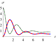
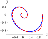
Figure 1: (a) The time evolutions of the (thick) position and (thin) momentum variances $\sigma_{x},\sigma_{p}$ for the correlated-(solid) and uncorrelated-(dashed) initial conditions with the finite Ohmic bath spectral density. (b) The $\bar{x}_{t}\bar{p}_{t}$-trajectories with the correlated-(solid) and uncorrelated-(dashed) initial conditions in the phase space. The parameters here are $\eta=0.5$, $k=1$, $\lambda=10$, and $x_{0}=1$.

In this section, we select some examples to show the utility of our exact results. At first, suppose the projective operator

$$f(x,p)=|\psi\rangle\langle\psi|,\quad|\psi\rangle=e^{-i\bar{x}_{0}p}e^{ir(xp+px)/2}|0\rangle$$ (53)

as the displaced squeezed state and $|0\rangle$ being the vacuum for free oscillator, is applied on the oscillator. The resulting initial state takes the factorized form,

$$\rho_{0}=|\psi\rangle\langle\psi|\otimes{\langle\psi|\rho_{T}|\psi\rangle\over Z},\quad Z=\mathrm{Tr}_{B}[\langle\psi|\rho_{T}|\psi\rangle].$$ (54)

This factorized state still captures the system-bath correlation by the classical dependence of the bath state on the system. Putting

$$\widetilde{f}_{w}(P,Q)=\exp\left[-\frac{1}{2}\left(\delta_{x}P^{2}+\delta_{p}Q^{2}\right)-i\bar{x}_{0}P\right],$$ (55)

associated with $\delta_{p}=\lambda/2$, $\delta_{x}=1/(2\lambda)$, and $\lambda=e^{2r}$ into (25) and calculating the four-fold integrals, we obtain

$$\widetilde{W}(P,Q,t) = \exp\bigg{[}-\frac{1}{2}\left(\sigma_{x}P^{2}+\dot{\sigma}_{x}PQ+\sigma_{p}Q^{2}\right)$$ (56)

$$-i\left(\bar{x}_{t}P+{\bar{p}}_{t}Q\right)\bigg{]},$$

where

$$\sigma_{x} = \langle x^{2}\rangle+{\lambda^{2}G^{2}+\dot{G}^{2}\over\lambda}-{(\dot{G}+2\lambda S)^{2}\over 2\lambda w_{x}}-{(\lambda G-2\dot{S})^{2}\over 2\lambda w_{p}},$$

$$\sigma_{p} = \langle p^{2}\rangle+{\lambda^{2}\dot{G}^{2}+\ddot{G}^{2}\over\lambda}-{(\ddot{G}+2\lambda\dot{S})^{2}\over 2\lambda w_{x}}-{(\lambda\dot{G}-2\ddot{S})^{2}\over 2\lambda w_{p}},$$

$$\bar{x}_{t} = {\dot{G}+2\lambda S\over w_{x}}\bar{x}_{0},\quad\bar{p}_{t}=\dot{\bar{x}}_{t},$$ (57)

with $w_{x}={1+4\delta_{p}\langle x^{2}\rangle}$, $w_{p}={1+4\delta_{x}\langle p^{2}\rangle}$, and $Z=\sqrt{w_{x}w_{p}}/2$. For the uncorrelated initial state

$$\rho_{0}=|\psi\rangle\langle\psi|\otimes\rho_{B}^{T},$$ (58)

the Wigner characteristic function is also given by Eq.(56) except with the different coefficients

$$\sigma_{x} = G^{2}\delta_{p}+\dot{G}^{2}\delta_{x}+b_{x},$$

$$\sigma_{p} = \dot{G}^{2}\delta_{p}+\ddot{G}^{2}\delta_{x}+b_{p}.$$

$$\bar{x}_{t} = \dot{G}\bar{x}_{0},\quad{\bar{p}}_{t}=\dot{\bar{x}}_{t}.$$ (59)

Figure 2: This plot shows the time evolutions of the purity $\mathrm{Tr}[\rho_{S}^{2}]$ with different squeezing parameters, $\lambda=10$ (solid), $1$ (dot-dashed), $0.1$ (dashed). The other parameters are chosen as in Fig. 1.

To see the implication of the above results, we resort to the numerical results pictorially. The parameters chosen for numerical computations are $\Lambda=10$ and $T=0$. In Fig. 1(a), we note for the factorized Gaussian states, the differences between the correlated and uncorrelated initial conditions are nearly unnoticeable for the evolutions of the position and momentum variances (54) and (58). However, the $\bar{x}_{t}\bar{p}_{t}$-trajectories in the phase space follow quite different pathes as displayed in Fig. 1(b). Such phenomena have also been observed in gauss before. More importantly, from Eqs. (57) and (59), this difference is still remarkable at high temperature because the correlation function $S(t)$ depends on temperature and for $T\gg\Lambda\gg\omega_{0}$, we have $\langle x^{2}\rangle\approx T/k$, $S(t)\approx{T/k}-T\int_{0}^{t}dt^{\prime}G(t^{\prime})$, and

$$\bar{x}_{t}\approx\bigg{[}1-k\int_{0}^{t}dt^{\prime}G(t^{\prime})\bigg{]}\bar{x}_{0}\neq\dot{G}\bar{x}_{0}.$$ (60)

Next, we consider the time evolution of the purity defined as $\sigma_{\mathrm{purity}}=\mathrm{Tr}[\rho_{S}^{2}]$, or

$$\sigma_{\mathrm{purity}}=\frac{1}{2\pi}\int d\Sigma|\widetilde{W}(P,Q,t)|^{2}=\frac{1}{\sqrt{4\sigma_{x}\sigma_{p}-\dot{\sigma}_{x}^{2}}}.$$ (61)

In Fig. 2, we see the appearance of the initial dips at short times due to the initial jolts hpz ; uz of the coefficients in the master equation. Therefore, the correlations among the factorized states are not enough to smooth out these dips. Because the purity does not sensitively depend on the initial conditions as shown above. We can use Eq. (59) to expand the purity at short times to find

$$\sigma_{\mathrm{purity}}\approx 1-\frac{\Lambda^{2}t^{2}}{2\pi\lambda},$$ (62)

which sharply decreases for times $t\ll\lambda^{1\over 2}/\Lambda$ as shown in Fig. 2. For long times, it approaches to the equilibrium value $\sigma_{\mathrm{purity}}=0.8658$. If we use the second way discussed in Sec. II to obtain an evolved state described by Eq. (31), the comparison of which with Eq. (59) and $\rho_{S}(0)$ characterized by Eq. (32) is shown in Fig. 3. It can be seen that they give different evolutions for the variance and purity. Particularly, we note that the initial dip associated with the factorized state does not show up for the new state, which dues to the correlation in the initial Gibbs state of the whole system is stronger than in the factorized initial state to smooth out the dip.

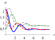
Figure 3: (a) The solid lines show the (thick) position and (thin) momentum variances $\sigma_{x},\sigma_{p}$ for the evolved state after the sudden change of the oscillating frequency $k=0.01\to\mathrm{k}=1$ at $t=0$. The dashed lines represent the relevant results under the uncorrelated initial condition. (b) The purity evolutions under the above two different conditions. Here $\sigma_{\mathrm{purity}}(0)=0.4870$ and $\eta=0.5$.

Figure 4: The plot of the survival probability ratio, $R=\mathrm{Pr}(2,1,0)/\mathrm{Pr}(2,0)$ versus the time interval $\tau$, for the exact-(solid) and approximated-(dashed) results with the (thick) intermediate coupling constant $\eta=0.5$ and (thin) weak coupling constant $\eta=0.1$. The spring constant is $k=1$.

Finally, we study the effects of two measurements $f_{j}=|0\rangle_{j}\langle 0|$ applied at times $t_{j}=j\tau$, $j=1,2$, during the evolution of the initial state prepared by $f_{0}=|0\rangle\langle 0|$ for simplicity. The quantities of interest are the joint conditional probabilities $\mathrm{Pr}(2,1|0)={\mathrm{Pr}(2,1,0)/\mathrm{Pr}(0)}$ and $\mathrm{Pr}(2|0)={\mathrm{Pr}(2,0)/\mathrm{Pr}(0)}$, which can be used to define the survival ratio

$$R={\mathrm{Pr}(2,1|0)\over\mathrm{Pr}(2|0)}={\langle f_{0}^{\dagger}f^{\dagger}_{1}f^{\dagger}_{2}f_{2}f_{1}f_{0}\rangle\over\langle f_{0}^{\dagger}f^{\dagger}_{2}f_{2}f_{0}\rangle}.$$ (63)

The meaning of $R>1$ ($R<1$) is that the intermediate measurement at $\tau$ enhances (suppresses) the survival probability of the initial state at $2\tau$, while $R=1$ indicates the crossover point. The explicit expression for $R$ involves the determination of a $10\times 10$ matrix, so it is too lengthy to put here and we only plot the numerical results in Fig. 4. A similar problem has been previously studied in zeno with the weak coupling and secular approximations to neglect the initial and subsequential oscillator-bath correlations and the fast oscillating terms in the master equation, respectively, and obtain a simplified equation for $\mathrm{Pr}(n,\dots,1|0)\approx\exp[-n\gamma(\tau)]$ with $\gamma(t)=\int_{0}^{t}dt^{\prime}D_{p}(t^{\prime})-{\omega_{0}/2}\int_{0}^{t}dt^{\prime}\Gamma(t^{\prime})$. From Fig. 4, we see that for the weak coupling $\eta=0.1$, the two results are almost the same. However, for a modest coupling $\eta=0.5$, they could become significantly different. Contrary to the conclusion in the weak coupling limit, the crossover points predicted by the exact results vary with the coupling constant sensitively, and are always less than the approximated ones.

VI Summary

In conclusion, we took the damped quantum harmonic oscillator as an example and applied the QLE and Wigner representation for operator to investigate the exact dynamics in the presence of the initial oscillator-bath correlation incorporated in two different ways: (i) prepare an initial state by a projective measurement on the oscillator; (ii) change the equation of motion of the oscillator by adjusting its parameters–mass or frequency initially. The simpler results thus obtained facilitate us to defy the possibility of the master equation independent of the initial state and specify several sufficient conditions resulting in some certain master equations. We also got a time-local QLE to derive the exact master equations under the factorized initial conditions, including the cases of initial correlated Gaussian states. It was shown that the variances of the factorized Gaussian states do not sensitively depend on the initial oscillator-bath correlations, which can however significantly influence the mean values even at high temperature. We demonstrated that the correlations among the factorized states still give rise to the initial dips during the purity evolutions, which can be smoothed out by increasing the amount of initial correlation to some extent. We finally studied the effects of repeated measurements on the evolution of the damped oscillator, which were compared with the weak coupling results to indicate that they give rather different transient behaviors even for an intermediate coupling.

APPENDIX

To introduce the Wigner representation of an arbitrary operator $A(x,p)$, let us first review the normal order of $A$, where $x$ is always put in front of $p$ in any product, denoting by $A=:A_{n}(x,p):$, such as $px=:xp-i:$. In particular, we can take $x,p$ as $c$-numbers inside the symbol $:$ $:$, i.e. $:xp:=:px:$. Inserting the unity decomposition, we have

$$A(x,p) = \int d\sigma^{\prime}|x^{\prime}\rangle\langle x^{\prime}|:A_{n}(x,p):|p^{\prime}\rangle\langle p^{\prime}|$$ (64)

$$= \int d\sigma^{\prime}|x^{\prime}\rangle\langle x^{\prime}|A_{n}(x^{\prime},p^{\prime})|p^{\prime}\rangle\langle p^{\prime}|$$

$$= \frac{1}{\sqrt{2\pi}}\int d\sigma^{\prime}|x^{\prime}\rangle\langle p^{\prime}|e^{ip^{\prime}x^{\prime}}A_{n}(x^{\prime},p^{\prime}),$$

and thus $A_{n}(x^{\prime},p^{\prime})=\sqrt{2\pi}\langle x^{\prime}|A(x,p)|p^{\prime}\rangle e^{-ip^{\prime}x^{\prime}}$. The composition rule $C(x,p)=A(x,p)B(x,p)$ can be transformed into

$$C(x,p) = \int d\sigma^{\prime}d\sigma^{\prime\prime}|x^{\prime}\rangle\langle x^{\prime}|A_{n}(x^{\prime},p^{\prime})|p^{\prime}\rangle\langle p^{\prime}|$$

$$\times|x^{\prime\prime}\rangle\langle x^{\prime\prime}|B_{n}(x^{\prime\prime},p^{\prime\prime})|p^{\prime\prime}\rangle\langle p^{\prime\prime}|$$

$$= \frac{1}{\sqrt{2\pi}}\int dx^{\prime}dp^{\prime\prime}|x^{\prime}\rangle\langle p^{\prime\prime}|e^{ip^{\prime\prime}x^{\prime}}C_{n}(x^{\prime},p^{\prime\prime}),$$

where

$$C_{n}(x^{\prime},p^{\prime\prime}) = \frac{1}{2\pi}\int dp^{\prime}dx^{\prime\prime}A_{n}(x^{\prime},p^{\prime})B_{n}(x^{\prime\prime},p^{\prime\prime})$$ (65)

$$\times e^{i(p^{\prime}-p^{\prime\prime})(x^{\prime}-x^{\prime\prime})}.$$

On the other hand, we have

$$A(x,p) = \int d\sigma^{\prime}A_{n}(x^{\prime},p^{\prime})\delta(x^{\prime}-x)\delta(p^{\prime}-p)$$ (66)

$$= \frac{1}{(2\pi)^{2}}\int d\sigma^{\prime}d\Sigma^{\prime}A_{n}(x^{\prime},p^{\prime})e^{iP^{\prime}(x-x^{\prime})}e^{iQ^{\prime}(p-p^{\prime})}$$

$$= \frac{1}{2\pi}\int d\Sigma^{\prime}\widetilde{A}_{n}(P^{\prime},Q^{\prime})e^{i(P^{\prime}x+Q^{\prime}p)-iP^{\prime}Q^{\prime}/2},$$

where we defined the normal order characteristic function

$$\widetilde{A}_{n}(P^{\prime},Q^{\prime}) = \frac{1}{2\pi}\int d\sigma^{\prime}A_{n}(x^{\prime},p^{\prime})e^{-i(P^{\prime}x^{\prime}+Q^{\prime}p^{\prime})}$$ (67)

$$= \mathrm{Tr}[Ae^{-i(P^{\prime}x+Q^{\prime}p)+iP^{\prime}Q^{\prime}/2}].$$

The appearances of $-iP^{\prime}Q^{\prime}/2$ in the last exponentials of (66) and (67) dues to the non-commutability of $x,p$. If we insist on omitting this term, the above equation should be re-interpreted as the Wigner representation or symmetrized order of the corresponding operator rather than the normal order, namely $A_{n}(x^{\prime},p^{\prime})\to A_{w}(x^{\prime},p^{\prime})$. In fact, they can be further generalized to

$$A(x,p) = \frac{1}{2\pi}\int d\Sigma^{\prime}\widetilde{A}_{g}(P^{\prime},Q^{\prime})e^{i(P^{\prime}x+Q^{\prime}p)-igP^{\prime}Q^{\prime}/2},$$

$$\widetilde{A}_{g}(P^{\prime},Q^{\prime}) = \frac{1}{2\pi}\int d\sigma^{\prime}A_{g}(x^{\prime},p^{\prime})e^{-i(P^{\prime}x^{\prime}+Q^{\prime}p^{\prime})}$$ (68)

$$= \mathrm{Tr}[Ae^{-i(P^{\prime}x+Q^{\prime}p)+igP^{\prime}Q^{\prime}/2}],$$

which includes the usual cases of $g=0$ or $\pm 1$ as the Wigner or (anti)-normal order representations.

As an example, take $A(x,p)=|0\rangle\langle 0|$, then $\langle x^{\prime}|0\rangle={e^{-x^{\prime 2}/2}/{\pi}^{1\over 4}}$, $\langle 0|p^{\prime}\rangle={e^{-p^{\prime 2}/2}/{\pi}^{1\over 4}}$, and

$$A_{n}=\sqrt{2\pi}\langle x^{\prime}|0\rangle\langle 0|{p^{\prime}}\rangle e^{-ip^{\prime}x^{\prime}}=\sqrt{2}e^{-(x^{\prime 2}+2ix^{\prime}p^{\prime}+p^{\prime 2})/2},$$

$$\widetilde{A}_{n}=e^{-(P^{\prime 2}+2iP^{\prime}Q^{\prime}+Q^{\prime 2})/4},\quad\widetilde{A}_{w}=e^{-(P^{\prime 2}+Q^{\prime 2})/4}.\hskip 17.07182pt$$ (69)

References

• (1) H.-P. Breuer and F. Petruccione, Open Quantum Systems (Oxford University Press, Oxford, 2002).
• (2) F. Haake and R. Reibold, Phys. Rev. A. 32, 2462 (1985).
• (3) B.L. Hu, J.P. Paz, and Y. Zhang, Phys. Rev. D. 45, 2843 (1992).
• (4) R. Karrlein and H. Grabert, Phys. Rev. E. 55, 153 (1997).
• (5) M.W.Y. Tu and W.M. Zhang, Phys. Rev. B 78, 235311 (2008); H.N. Xiong, W.M. Zhang, X. Wang, and M.H. Wu, Phys. Rev. A 82, 012105 (2010); W.M. Zhang, P.Y. Lo, H.N. Xiong, M.W.Y. Tu, and F. Nori, Phys. Rev. Lett. 109, 170402 (2012).
• (6) K. Modi and E.C.G. Sudarshan, Phys. Rev. A. 81, 052119 (2010).
• (7) E.-M. Laine, J. Piilo, and H.-P. Breuer, Europhys. Lett. 92, 60010 (2010); J. Dajka and J. Luczka, Phys. Rev. A. 82, 012341 (2010).
• (8) H.T. Tan and W.M. Zhang, Phys. Rev. A. 83, 032102 (2011); V.G. Morozov, S. Mathey, and G. Röpke, Phys. Rev. A 85, 022101 (2012); Y. Gao, Euro. Phys. J. D 67, 183 (2013).
• (9) G.W. Ford and R.F. O’Connell, Phys. Rev. A. 76, 042122 (2007).
• (10) C.M. Smith and A.O. Caldeira, Phys. Rev. A. 36, 3509 (1987); ibid. 41, 3103 (1990).
• (11) W.G. Unruh and W.H. Zurek, Phys. Rev. D. 40, 1071 (1989);
• (12) G.W. Ford, J.T. Lewis, and R.F. O’Connell, Phys. Rev. A. 37, 4419 (1988).
• (13) G.W. Ford and R.F. O’Connell, Phys. Rev. D. 64, 105020 (2001); Ann. Phys. 319, 348 (2005).
• (14) H.B. Callen and T.A. Welton, Phys. Rev. 83, 34 (1951).
• (15) L.D. Romero and J.P. Paz, Phys. Rev. A. 55, 4070 (1997).
• (16) C.H. Fleming, A. Roura, and B.L. Hu, Ann. Phys. 326, 1207 (2011).
• (17) E. Pollak, J. Shao, and D.H. Zhang, Phys. Rev. E. 77, 021107 (2008).
• (18) S. Maniscalco, J. Piilo, and K.A. Suominen, Phys. Rev. Lett. 97, 130402 (2006).