PRESSURE OF DEGENERATE AND RELATIVISTIC ELECTRONS IN A SUPERHIGH MAGNETIC FIELD

Abstract

Based on our previous work, we deduce a general formula for pressure of degenerate and relativistic electrons, $P_{e}$, which is suitable for superhigh magnetic fields, discuss the quantization of Landau levels of electrons, and consider the quantum electrodynamic(QED) effects on the equations of states (EOSs) for different matter systems. The main conclusions are as follows: $P_{e}$ is related to the magnetic field $B$, matter density $\rho$, and electron fraction $Y_{e}$; the stronger the magnetic field, the higher the electron pressure becomes; the high electron pressure could be caused by high Fermi energy of electrons in a superhigh magnetic field; compared with a common radio pulsar, a magnetar could be a more compact oblate spheroid-like deformed neutron star due to the anisotropic total pressure; and an increase in the maximum mass of a magnetar is expected because of the positive contribution of the magnetic field energy to the EOS of the star.

Received (Day Month Year)Revised (Day Month Year)

PACS: 71.70.Di; 97.0.L.d; 71.18.+y.

1 Introduction

Thompson and Duncan (1996) predicted that superhigh magnetic fields could exist in the interiors of magnetars, which are powered by extremely strong magnetic fields, $B\sim 10^{14}$ to $10^{15}$ G (see Ref. Thompson96). The majority of magnetars are classified into two populations historically: the soft gamma-ray repeaters (SGRs), and the anomalous X-ray pulsars (AXPs). Pulsars have been recognized to be normal neutron stars (NSs), but sometimes have been argued to be quark stars (e.g., see Ref. Xu02, Xu05,  Du09).

It is universally accepted that ${}^{3}P_{2}$ anisotropic neutron superfluid could exist in the interior of a neutron star (NS). If the superhigh magnetic fields of magnetars originate from the magnetic fields induced by the ferromagnetic moments of the ${}^{3}P_{2}$ Cooper pairs of the anisotropic neutron superfluid at a moderate to lower temperatures ($T\ll 2.87\times 10^{8}$ K, the critical temperature of the ${}^{3}P_{2}$ neutron superfluid) and high nuclear density ($\sim 0.5\rho_{0}<\rho<2.0\rho_{0}$), then the maximum magnetic field strength for the heaviest magnetar may be estimated to be $(3.0\sim 4.0)\times 10^{15}$ G, according to our model (see Ref. Peng07, Peng09).

For completely degenerate ($T\rightarrow 0$, i.e., $\mu/kT\rightarrow\infty$, $\mu$ is the chemical potential of species $i$, also called the Fermi energy, $E_{\rm F}(i)$) and relativistic electrons in equilibrium, the distribution function $f(E_{e})$ can be expressed as

$$f(E_{e})=\frac{1}{Exp[(E_{e}-\mu_{e})/kT]+1}~{}~{},~{}~{}$$ (1)

where the sign $+$ refers to Fermi-Dirac statistics, $k$ represents Boltzmann’s constant; and $\mu_{e}$ is the electron chemical potential; when $E_{e}\leq E_{\rm F}(e),f(E_{e})=1$; when $E_{e}>E_{\rm F}(e)$, $f(E_{e})=0$. The electron Fermi energy $E_{\rm F}(e)$ has the simple form

$$E_{\rm F}^{2}(e)=p^{2}_{\rm F}(e)c^{2}+m^{2}_{e}c^{4}~{}~{},~{}~{}$$ (2)

with $p_{\rm F}(e)$ being the electron Fermi momentum.

In the interior of a NS, when $B$ is too weak to be taken into consideration, $p_{\rm F}(e)$, is mainly determined by matter density $\rho$ and the electron fraction $Y_{e}$ (see Ref. Shapiro83). In the weak-field limit $B^{*}\ll 1$ (${B^{*}=B/B_{\rm cr}}$ and $B_{\rm cr}=4.414\times 10^{13}$ G is the electron critical field), the equation of state (EOS) can be written in the polytropic form,

$$P_{e}=K\rho^{\Gamma}~{}~{},~{}~{}$$ (3)

where $K$ and $\Gamma$ are constants, in the following two limiting cases: 1.For non-relativistic electrons, $\rho\ll 10^{6}$ g cm^-3,

$$\Gamma=\frac{5}{3},~{}~{}K=\frac{1.0036\times 10^{13}}{(A/Z)^{5/3}}~{}~{}~{}{\rm cgs}~{}~{},~{}~{}$$ (4)

where $A$ and $Z$ are the number of nucleons and the number of protons, respectively. 2. For extremely relativistic electrons, $\rho\gg 10^{6}$ g cm^-3,

$$\Gamma=\frac{4}{3},~{}~{}~{}K=\frac{1.2435\times 10^{15}}{(A/Z)^{4/3}}~{}~{}~{}~{}~{}{\rm cgs}~{}.~{}~{}$$ (5)

Be note that, for a given nucleus with proton number $Z$ and nucleon number $A$, the relation of $Y_{e}=Y_{p}=Z/A$ always approximately holds, where $Y_{p}$ is the proton fraction; for an ideal neutron-proton-electron ($npe$) gas, $Y_{e}=Y_{p}=\frac{n_{e}}{n_{B}}=\frac{n_{e}}{n_{p}+n_{n}}\approx\frac{n_{e}}{n_{n}}$, where $n_{e}$, $n_{p}$, $n_{n}$ and $n_{B}$ are the electron number density, proton number density, neutron number density and baryon number density, respectively.

In this paper, we focus on the interior of a magnetar where electrons are degenerate and relativistic. The effects of a strong magnetic field on the equilibrium composition of a NS have been shown in detail in previous studies (e.g., Ref. Yakovlev01, Lai91). In accordance with the popular point of view on the electron pressure in strong magnetic fields, the stronger the magnetic field, the lower the electron pressure becomes. With respect to this viewpoint, we cannot directly verify it by the experiment in actual existence, owing to the lack of such high-value magnetic fields on the earth. After a careful check, we found that popular methods of calculating the Fermi energy of electrons are contradictory to the quantization of electron Landau levels. In an extremely strong magnetic field, the Landau column becomes a very long and very narrow cylinder along the magnetic field. By introducing the Dirac $\delta$-function, we obtain

$$\frac{4\pi}{3B^{*}}(\frac{m_{e}c}{h})^{3}(\gamma_{e})^{4}\int_{0}^{1}(1-\frac{1}{\gamma^{2}_{e}}-\chi^{2})^{\frac{3}{2}}d\chi-2\pi\gamma_{e}(\frac{m_{e}c}{h})^{3}\sqrt{2B{*}}=N_{A}\rho Y_{e}~{}~{},~{}~{}$$ (6)

where $\chi$ and $\gamma_{e}$ are two non-dimensional variables, defined as $\chi=(\frac{p_{z}}{m_{e}c})/(\frac{E_{\rm F}(e)}{m_{e}c^{2}})=p_{z}c/E_{\rm F}(e)$ and $\gamma_{e}=E_{\rm F}(e)/m_{e}c^{2}$, respectively; $1/\gamma^{2}_{e}$ is the modification factor; $h$ and $N_{A}$ are the Planck constant and Avogadro constant, respectively (see Ref.  Gao11a, Gao12a). Solving Eq.(6) gives a concise formula for $E_{\rm F}(e)$ in superhigh magnetic fields,

$$E_{\rm F}(e)\simeq 43.44(\frac{B}{B_{\rm cr}})^{1/4}(\frac{\rho}{\rho_{0}}\frac{Y_{e}}{0.0535})^{\frac{1}{4}}~{}~{}~{}~{}~{}\rm MeV~{}~{},~{}$$ (7)

where $\rho_{0}=2.8\times 10^{14}$ g cm³ is the standard nuclear density (see Ref. Gao12a).

The remainder of this paper is organized as follows: in Section 2, on the basis of our previous work, we deduce an equation involving $P_{e}$, $\rho$, $B$ and $Y_{\rm e}$, which is suitable for strong magnetic fields; in Section 3, we take into account QED effects on EOSs of different matter systems, and discuss an anisotropy of the total pressure of ideal $npe$ gas due to strong magnetic fields; in Section 4, we present a dispute on $P_{e}$ in superhigh magnetic fields, and finally we summarize our findings with conclusions in Section 5.

2 Pressure of degenerate and relativistic electrons

The relativistic Dirac-Equation for the electrons in a uniform external magnetic field along the $z-$axis gives the electron energy level

$$E_{e}=[m_{e}^{2}c^{4}(1+\nu\frac{2B}{B_{\rm cr}})+p^{2}_{z}c^{2}]^{\frac{1}{2}}~{}~{},~{}~{}$$ (8)

where the quantum number $\nu$ is given by $\nu=n+\frac{1}{2}+\sigma$ for the Landau level $n=0,1,2,\cdots$, spin $\sigma=\pm\frac{1}{2}$ (see Ref. Canuto77), and the quantity $p_{z}$ is the $z$-component of the electron momentum and may be treated as a continuous function. Combining $B_{\rm cr}=m^{2}_{e}c^{3}/{e}\hbar$ with $\mu_{e}^{{}^{\prime}}=e\hbar/2m_{e}c$ gives

$$E_{e}^{2}=m_{e}^{2}c^{4}+p_{z}^{2}c^{2}+2\nu 2m_{e}c^{2}\mu_{e}^{{}^{\prime}}B~{}~{},~{}~{}$$ (9)

where $\mu_{e}^{{}^{\prime}}$ is the magnetic moment of an electron.

For the convenience of the following calculations, we define the electron momentum perpendicular to the magnetic field, $p_{\bot}=m_{e}c(2\nu B^{*})^{\frac{1}{2}})$. Then, Eq.(9) can be rewritten as,

$$E_{e}^{2}=m_{e}^{2}c^{4}+p_{z}^{2}c^{2}+p_{\bot}^{2}c^{2}~{}~{},~{}~{}$$ (10)

The maximum electron Landau level number $n_{max}$ is uniquely determined by the condition $[p_{\rm F}(z)c]^{2}\geq 0$ (see Ref. Lai91), where $p_{\rm F}(z)$ is the Fermi momentum along the $z-$axis. The expression for $n_{max}$ is

$$n_{\rm max}(\sigma=-\frac{1}{2})=Int[\frac{1}{2B^{*}}[(\frac{E_{\rm F}(e)}{m_{e}c^{2}})^{2}-1-(\frac{p_{z}}{m_{e}c})^{2}]]~{}~{},$$

$$n_{\rm max}(\sigma=~{}\frac{1}{2})=Int[\frac{1}{2B^{*}}[(\frac{E_{\rm F}(e)}{m_{e}c^{2}})^{2}-1-(\frac{p_{z}}{m_{e}c})^{2}]-1]~{}~{},~{}~{}$$ (11)

where $Int[x]$ denotes an integer value of the argument $x$. Correspondingly, the expression for $\nu_{max}$ can be expressed as

$$\nu_{max}(\sigma=-\frac{1}{2})=Int[\frac{1}{2B^{*}}[(\frac{E_{\rm F}(e)}{m_{e}c^{2}})^{2}-1-(\frac{p_{z}}{m_{e}c})^{2}]+\frac{1}{2}-\frac{1}{2}]~{}~{},$$

$$=Int[\frac{1}{2B^{*}}[(\frac{E_{\rm F}(e)}{m_{e}c^{2}})^{2}-1-(\frac{p_{z}}{m_{e}c})^{2}]]~{}~{},$$

$$\nu_{max}(\sigma=\frac{1}{2})=Int[\frac{1}{2B^{*}}[(\frac{E_{\rm F}(e)}{m_{e}c^{2}})^{2}-1-(\frac{p_{z}}{m_{\rm e}c})^{2}]-1+\frac{1}{2}+~{}\frac{1}{2}]~{}~{},$$

$$=Int[\frac{1}{2B^{*}}[(\frac{E_{\rm F}(e)}{m_{e}c^{2}})^{2}-1-(\frac{p_{z}}{m_{e}c})^{2}]]~{}~{}.~{}~{}$$ (12)

From Eq.(12), it’s obvious that

$$\nu_{max}(\sigma=-\frac{1}{2})=\nu_{max}(\sigma=\frac{1}{2}).$$ (13)

However, the electron Fermi momentum is the maximum of electron momentum. The physics on the condition $[p_{\rm F}(z)c]^{2}\geq 0$ in Ref. Lai91 includes that: $n_{max}$ is determined by $E_{\rm F}(e)$ and $p_{z}$ when $B$ is given; for a given Landau level number $n$, $p_{z}$ always has the maximum $p_{z}(max)$ corresponding to $n$; in the same way, when $p_{z}$ is given, $n$ also has the maximum $n_{max}$ corresponding to $p_{z}$. Maybe $n_{max}^{{}^{\prime}}$ corresponding to $p_{z}~{}=~{}0$ is most meaningful to us, and so is $p_{\rm F}(z)$ corresponding to $n~{}=0$ (when $n=0$, the spin is antiparallel to $B$,and $\sigma~{}=-\frac{1}{2}$).

According to the definition of $E_{\rm F}(e)$ in Eq.(2), we obtain $E_{\rm F}(e)\equiv p_{\rm F}(e)c$ if electrons are super-relativistic ($E_{\rm F}(e)\gg m_{e}c^{2}$). In the presence of a superhigh magnetic field $B\gg B_{\rm cr}$, $E_{\rm F}(e)\gg m_{e}c^{2}$), hence we have the following approximate relation

$$\nu_{max}(\sigma=-\frac{1}{2})^{{}^{\prime}}=~{}\nu_{max}(\sigma=~{}\frac{1}{2})^{{}^{\prime}}\simeq Int[\frac{1}{2B^{*}}[(\frac{E_{\rm F}(e)}{m_{e}c^{2}})^{2}]~{}~{}.~{}~{}$$ (14)

From the analysis above, we can calculate the maximum of electron momentum perpendicular to the magnetic field by

$$p_{\bot}^{2}(max)c^{2}=~{}2\nu_{max}^{{}^{\prime}}2m_{e}c^{2}\mu_{e}^{{}^{\prime}}B~{}~{},~{}~{}$$ (15)

where the relation of $2\mu_{e}^{{}^{\prime}}B_{\rm cr}/m_{e}c^{2}=1$ is used. Inserting Eq.(14) into Eq.(15) gives

$$p_{\bot}^{2}(max)c^{2}=~{}2\times\frac{1}{2B^{*}}(\frac{E_{\rm F}(e)}{m_{e}c^{2}})^{2}\times 2m_{e}c^{2}\mu_{e}^{{}^{\prime}}B$$

$$\simeq B_{\rm cr}\times(\frac{E_{\rm F}(e)}{m_{e}c^{2}})^{2}\times 2m_{e}c^{2}\frac{e\hbar}{2m_{e}c}$$

$$=\frac{m_{e}^{2}c^{3}}{e\hbar}\times(\frac{E_{\rm F}(e)}{m_{e}c^{2}})^{2}\times 2m_{e}c^{2}\frac{e\hbar}{2m_{e}c}=~{}E_{\rm F}^{2}(e)~{}~{}.~{}~{}$$ (16)

Thus, we gain

$$p_{\bot}(max)=p_{\rm F}(e)\simeq\frac{E_{\rm F}(e}{c}$$

$$=43.44\times(\frac{Y_{e}}{0.0535}\frac{\rho}{\rho_{0}}\frac{B}{B_{\rm cr}})^{\frac{1}{4}}{\rm MeV/c}~{}(B^{*}\geq 1~{})~{}~{}.~{}~{}$$ (17)

As pointed out above, when $n=0$, the electron Landau level is non-degenerate, and $p_{z}$ has its maximum $p_{z}(max)$,

$$p_{z}(max)=p_{\rm F}(e)\simeq\frac{E_{\rm F}(e)}{c}$$

$$=43.44\times(\frac{Y_{e}}{0.0535}\frac{\rho}{\rho_{0}}\frac{B}{B_{\rm cr}})^{\frac{1}{4}}{\rm MeV/c}~{}(B^{*}\geq 1~{})~{}~{}.~{}~{}$$ (18)

From Eq.(17) and Eq.(18), it’s obvious that $p_{z}(max)=p_{\bot}(max)=p_{\rm F}(e)$, which implies the electron pressure along the magnetic field, $P_{z}(e)$, is equal to the electron pressure in the direction perpendicular to the magnetic field, $P_{\bot}(e)$. The reason for this is that in the interior of a magnetar, electrons are degenerate and super-relativistic, and can be approximately treated as an ideal Fermi gas with equivalent pressures in all directions, though the existence of Landau levels. The equation of $P_{e}$ in a superhigh magnetic field is consequently given by

$$P_{e}=\frac{1}{3}\frac{2}{h^{3}}\int_{0}^{p_{\rm F}(e)}\frac{p_{e}^{2}c^{2}}{(p_{e}^{2}c^{2}+m_{e}^{2}c^{4})^{1/2}}4\pi p_{e}^{2}dp_{e}$$

$$=\frac{m_{e}c^{2}}{\lambda_{e}^{3}}\phi(x_{e})=1.412\times 10^{25}\phi(x_{e})~{}~{}{\rm dynes~{}cm^{-2}}~{}~{},~{}~{}$$ (19)

where $\lambda_{e}=\frac{h}{m_{e}c}$ is the electron Compton wavelength, and $\phi(x_{e})$ is the polynomial of a non-dimensional variable $x_{e}$ ($x_{e}=\frac{p_{\rm F}(e)}{m_{e}c}\simeq\frac{E_{\rm F}(e)}{m_{e}c^{2}}=86.77\times(\frac{\rho}{\rho_{0}}\frac{B}{B_{\rm cr}}\frac{Y_{e}}{0.0535})^{\frac{1}{4}}$),

$$\phi(x_{e})=\frac{1}{8\pi^{2}}[x_{e}(1+x_{e}^{2})^{\frac{1}{2}}(\frac{2x_{e}^{2}}{3}-1)+ln[x_{e}+(1+x_{e}^{2})^{\frac{1}{2}}]]~{}~{}.~{}~{}$$ (20)

When $\rho\geq 10^{7}$ g cm^-3, $x_{e}\gg 1$, and $\phi(x_{e})\rightarrow\frac{x_{e}^{4}}{12\pi^{2}}$. Thus, Eq.(19) can be rewritten as

$$P_{e}\simeq 6.266\times 10^{30}(\frac{\rho}{\rho_{0}}\frac{B}{B_{\rm cr}}\frac{Y_{e}}{0.0535})~{}~{}{\rm dyne~{}cm^{-2}}~{}~{}.~{}~{}.$$ (21)

Comparing Eq.(21) with Eq.(7), it’s easy to see that $P_{e}\propto E_{\rm F}^{4}(e)$. Employing Eq.(21), we plot the schematic diagrams of $P_{e}$ vs. $B$, as shown in Fig.1.

file=Fig.1.eps,width=4.0in

Figure 1: The electron pressure dependence of the magnetic field strength when $\rho=\rho_{0}$ and $Y_{e}=0.06$. When $B$ is assumed to be $(1.0\times 10^{14}\sim 3.0\times 10^{15}$) G, $P_{e}$ is $(1.592\times 10^{31}\sim 4.776\times 10^{32}$ dynes cm^-2), correspondingly.

From Fig.1, $P_{e}$ increases sharply with increasing $B$ when the values of $Y_{e}$ and $\rho$ are given. We also present a schematic illustration of $P_{e}$ as a function of $\rho$ in different magnetic fields, as shown in Fig.2.

file=Fig.2.eps,width=4.0in

Figure 2: The electron pressure dependence of the matter density in different magnetic fields when $Y_{e}=0.06$. When $\rho$ is assumed to be $(1.0\times 10^{14}\sim 5.6\times 10^{14}$) g cm^-3, the ranges of $P_{e}$ are $1.471\times 10^{30}\sim 1.454\times 10^{32}$ dynes cm^-2,$3.411\times 10^{31}\sim 1.910\times 10^{32}$ dynes cm^-2, and $1.521\times 10^{32}\sim 8.545\times 10^{32}$ dynes cm^-2, respectively, corresponding to $B^{*}\ll 1$, $B=~{}6.0\times 10^{14}$ G and $B=3.0\times 10^{15}$ G, respectively. The solid line is obtained from Eq.(3) for the relativistic electrons (see Section 1).

As pointed in our previous study (see Ref. Gao11a), the high Fermi energy of electrons could be supplied by the release of the magnetic field energy. Since $P_{e}$ is proportional to $E_{\rm F}^{4}(e)$, and the later increases with increasing $B$, then the former also increases with increasing $B$ naturally. Although we have presented a reasonable explanation for high-value $P_{e}$ here, an important issue of electron distributions among different Landau levels in a superhigh magnetic field remains unsolved. According to a popular viewpoint that the stronger the magnetic field, the smaller the maximum electron Landau level number $n_{max}$ becomes, the number of electrons congregating in an exciting level ($n\geq 1$) decrease with increasing $B$, if $B\gg B_{\rm cr}$, then $n_{max}=~{}1$ or 2, and the overwhelming majority of electrons occupy in the ground level $n=~{}0$, which causes a decrease in the momentum $p_{z}$, as well as a decrease in the momentum $p_{\bot}$. However, the Dirac Delta-function $\delta(\frac{p_{\bot}}{m_{e}c}-[2(n+\sigma+\frac{1}{2})B^{*}]^{\frac{1}{2}})$ obviously tells us that, given a Landau level number $n$, both the momentum $p_{\bot}(n)\sim m_{e}c[2(n+\sigma+\frac{1}{2})B^{*}]^{\frac{1}{2}}$ and the magnetic energy $E_{B}(n)\sim p_{\bot}(n)c\sim m_{e}c^{2}[2(n+\sigma+\frac{1}{2})B^{*}]^{\frac{1}{2}}$ increase with increasing $B$, which implies more electrons contribute to $p_{\bot}(n)$ and $E_{B}(n)$. Thus, given a Landau level $n$, the number of electrons should increase with increasing $B$, rather than decrease with $B$. With respect to $\Delta p_{\bot}(n,n+1)$, the difference of $p_{\bot}$ between two adjacent landau levels, when the Landau level number $n$ is given, $\Delta p_{\bot}(n,n+1)$ increases with increasing $B$; when $B$ is given, $\Delta p_{\bot}(n,n+1)$ decreases with increasing $n$, and if $n\rightarrow n_{max}$, then $\Delta p_{\bot}(n,n+1)$ is too small to be taken into account. The increase of $E_{\rm F}(e)$, together with the increase of number of electrons populating in the vicinity of Fermi surface, can result in an increase in the electron capture(EC) rate in the interior of a magnetar. The extreme activity and instability of a magnetar may be explained by high-value $E_{\rm F}(e)$, and the released thermal energy in the EC process could be the source of magnetars’ soft X/$\gamma$-ray radiations (see Ref. Gao12a, Gao11b, Gao12b).

3 The QED effects on equation of state

A superhigh magnetic field is intriguing in the physical context because some interesting phenomena would be expected from the quantum electrodynamic (QED) effects. One of the QED phenomena is the vacuum polarization, which causes large energy splitting of Landau levels, modifies the dielectric properties of the medium, induces resonant conversion of photon modes (e.g., see Ref. Ventura79, Bulik97, Kohri02),and decreases the equivalent width of the ion cyclotron line making the line more difficult to observe (see Ref. Ho03).

The observations display the presence of the hard X-ray spectra tails in magnetars, recently detected by XMM, ASCA, RXTE and INTEGRAL (e.g., see Ref. Kuiper04,  Molkov05, Mereghetti05, Gotz06, Kuiper06, den Hartog08). Some authors have tried to interpret these observations by employing Resonant Compton Scattering (RCS) by relativistic electrons in superhigh magnetic fields (e.g., see Ref. Lyutikov06, Baring07, Rea08,  Nobili08, Baring11, Gonthier12). RCS is also an interesting phenomenon due to QED effects, and has been treated as a leading emission mechanism for the hard X-ray radiation of magnetars. With respect to the QED effects on the spin-down and heat evolution of magnetars, for details, see a recent review of Ref. Battesti13.

However, as an alternative, in this work, we shall concentrate on the QED effects on different matter systems of a magnetar, and discuss the star’s deformation due to strong magnetic fields. This Section is composed of three sub-sections. For each subsection we present different methods and considerations.

3.1 The QED effects on the EOS of BPS model

Considering shell effects on the binding energy of a given nucleus, Salpeter (1961) first calculated the composition and EOS in the region of $10^{7}-3.4\times 10^{11}$ g cm^-3 (see Ref. Salpeter61). By introducing the lattice energy, Baym, Pethick and Sutherland (hereafter BPS model) improved on Salpeter’s treatment, and described the nuclear composition and EOS for catalyzed matter in complete thermodynamic equilibrium below neutron drop $\rho_{d}\sim 4.4\times 10^{11}$ g cm^-3 energy (see Ref. BPS71, Shapiro83).

Here, we shall not discuss electrons in the low density regime $10^{4}\sim 10^{6}$ g  cm^-3, because the electrons are nonrelativistic, and EOS may be treated via a magnetic Thomas-Fermi (TF) type of model for a lattice of electrons and ${}^{56}_{26}Fe$ nuclei (see Ref. Fushiki89). Since we are concerned about the role of magnetic fields on EOS, a qualitative analysis of magnetic influence depending on the details of the nuclear model will not be presented here. Also, we’ll utilize the simple BPS model, and no long consider other more complicated models (e.g., the model in Ref. Haensel89, in which the EOS is quite distinct from that of BPS model). We’ll assume an isotropic and homogenous matter pressure $P$ of this system. An anisotropy of the total pressure $P_{tot}$ of the system due to a strong magnetic field will not be discussed in this subsection.

According to BPS model, the matter energy density is given by

$$\varepsilon=n_{N}(W_{N}(A,Z)+\varepsilon_{L}(Z,n_{e})+\varepsilon_{e}(n_{e})~{}~{},~{}~{}$$ (22)

where $n_{N}$ is the number density of nuclei, $W_{N}(A,Z)$ is the mass- energy per nucleus (including the rest mass of $Z$ electrons and $A$ nucleons); $\varepsilon_{e}$ is the free electron energy including the rest mass of electrons in a unit volume; $\varepsilon_{L}$ is the $bcc$ Coulomb lattice energy per nucleus,

$$\varepsilon_{L}=-1.444Z^{2/3}e^{2}e^{2}n_{e}^{4/3}~{}~{},~{}~{}$$ (23)

where the relations of $n_{N}=~{}n_{B}/A$ and $n_{e}=~{}Zn_{N}$ are used. The matter pressure $p$ of the system is given by

$$P=P_{e}+P_{L}=P_{e}+\frac{1}{3}\varepsilon_{L}~{}~{}.~{}~{}$$ (24)

In the case of the weak-field limit $B^{*}\ll 1$, $P_{e}$ in Eq.(24) is given by Eq.(5). For a magnetic field $B^{*}\gg 1$, $P_{e}$ in Eq.(24) is given by Eq.(21). For the specific equilibrium nuclei $(A,Z)$ in BPS model, we calculate the values of quantities $\rho_{m}$, $n_{B}(m)$, $E_{\rm F}(e)$ and $P_{e}$, as tabulated in Table 1.

Values of $\rho_{m}$, $n_{B}(m)$, $E_{\rm F}(e)$ and $P_{e}$ in BPS model below neutron drip. Nuclei^† $Y_{e}$ $\rho_{m}^{0}$ $\rho_{m}^{1}$ $n_{B}^{0}(m)$ $n_{B}^{1}(m)$ $E_{\rm F}^{0}(e)$ $E_{\rm F}^{1}(e)$ $P_{e}^{0}$ $P_{e}^{1}$ g cm^-3 g cm^-3 cm^-3 cm^-3 MeV MeV dynes cm^-2 dynes cm^-2 ${}^{56}_{26}Fe$ 0.464 7.99$\times 10^{6}$ 4.67$\times 10^{8}$ 4.812$\times 10^{30}$ 2.812$\times 10^{32}$ 0.95 8.77 7.141$\times 10^{23}$ 9.069$\times 10^{27}$ ${}^{62}_{28}Ni$ 0.452 2.71$\times 10^{8}$ 1.68$\times 10^{9}$ 1.632$\times 10^{32}$ 1.012$\times 10^{33}$ 2.61 12.01 7.556$\times 10^{25}$ 3.174$\times 10^{28}$ ${}^{64}_{28}Ni$ 0.437 1.31$\times 10^{9}$ 2.78$\times 10^{9}$ 7.949$\times 10^{32}$ 1.674$\times 10^{33}$ 4.31 13.59 5.980$\times 10^{26}$ 5.087$\times 10^{28}$ ${}^{66}_{28}Ni$ 0.424 1.54$\times 10^{9}$ No^‡ 9.274$\times 10^{32}$ No^‡ 4.45 No^‡ 7.049$\times 10^{26}$ No^‡ ${}^{86}_{36}Kr$ 0.419 3.11$\times 10^{9}$ 3.87$\times 10^{9}$ 1.873$\times 10^{33}$ 2.331$\times 10^{33}$ 5.66 14.49 1.767$\times 10^{27}$ 6.776$\times 10^{28}$ ${}^{84}_{34}Se$ 0.405 9.98$\times 10^{9}$ 1.14$\times 10^{10}$ 6.009$\times 10^{33}$ 6.865$\times 10^{33}$ 8.49 18.84 7.999$\times 10^{27}$ 1.930$\times 10^{29}$ ${}^{82}_{32}Ge$ 0.390 2.08$\times 10^{10}$ 2.10$\times 10^{10}$ 1.252$\times 10^{34}$ 1.265$\times 10^{34}$ 11.44 21.75 2.028$\times 10^{28}$ 3.428$\times 10^{29}$ ${}^{80}_{30}Zn$ 0.375 5.91$\times 10^{10}$ 5.69$\times 10^{10}$ 3.559$\times 10^{34}$ 3.426$\times 10^{34}$ 14.08 27.62 7.741$\times 10^{28}$ 8.925$\times 10^{29}$ ${}^{78}_{28}Ni$ 0.359 8.21$\times 10^{10}$ 8.13$\times 10^{10}$ 4.944$\times 10^{34}$ 4.896$\times 10^{34}$ 20.01 28.86 1.132$\times 10^{29}$ 1.221$\times 10^{30}$ ${}^{126}_{44}Ru$ 0.349 1.19$\times 10^{11}$ 1.20$\times 10^{11}$ 7.166$\times 10^{34}$ 7.226$\times 10^{34}$ 20.20 31.59 1.789$\times 10^{29}$ 1.753$\times 10^{30}$ ${}^{124}_{42}Mo$ 0.339 1.66$\times 10^{11}$ 1.67$\times 10^{11}$ 9.996$\times 10^{34}$ 1.006$\times 10^{35}$ 20.50 34.05 2.678$\times 10^{29}$ 2.366$\times 10^{30}$ ${}^{122}_{40}Zr$ 0.328 2.49$\times 10^{11}$ 2.50$\times 10^{11}$ 1.499$\times 10^{35}$ 1.506$\times 10^{35}$ 22.89 37.32 4.404$\times 10^{29}$ 2.428$\times 10^{30}$ ${}^{120}_{38}Sr$ 0.317 3.67$\times 10^{11}$ 3.08$\times 10^{11}$ 2.210$\times 10^{35}$ 2.216$\times 10^{35}$ 25.20 40.77 7.052$\times 10^{29}$ 4.871$\times 10^{30}$ ${}^{122}_{38}Sr$ 0.311 3.89$\times 10^{11}$ 3.90$\times 10^{11}$ 2.342$\times 10^{35}$ 2.348$\times 10^{35}$ 25.90 41.20 7.455$\times 10^{29}$ 5.120$\times 10^{30}$ ${}^{118}_{36}Kr$ 0.305 4.41$\times 10^{11}$ 4.41$\times 10^{11}$ 2.656$\times 10^{35}$ 2.656$\times 10^{35}$ 26.20 42.28 7.805$\times 10^{29}$ 5.692$\times 10^{30}$

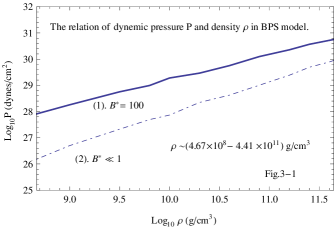
In this Table the signs of $`0^{\prime}$ and $`1^{\prime}$ denote $B^{*}\ll 1$ and $B^{*}=100$, respectively, and $n_{B}(m)$ is the maximum equilibrium baryon number density, corresponding to the maximum equilibrium density $\rho_{m}$ at which the nuclide is present. The sign $`{\dagger}^{\prime}$ denotes that the first masses are known experimentally (see Ref. Wapstra77), and the remainder are from the Jäanecke-Gravey-Kelson mass formula (see Ref. Wapstra76). The sign $`{\ddagger}^{\prime}$ denotes that ${}^{62}_{28}Ni$ is found to be absent from the equilibrium nucleus sequence, so is not presented. Furthermore, all digits in Column 3 and Column 4 of this Table are cited from Lai and Shapiro (1991) (see Ref. Lai91). From Table 1, it’s obvious that the electron pressure $P_{e}$, as well as $E_{\rm F}(e)$, increases with matter density and magnetic field, and a strong magenetic field alters the nucleus transition densities for the low-$A$ nuclei. In a strong magnetic field, as the density increases, the nuclei become increasingly saturated with neutrons, however, neutron drip occurs at the same density because we adopts a nearly constant minimum Gibbs free energy per nucleon, $g_{min}=m_{n}c^{2}$. From Table 1, the calculated values of $P_{e}$ are in the range of $9.069\times 10^{27}\sim 5.692\times 10^{30}$ dynes cm^-2 corresponding to a density range of $4.67\times 10^{8}\sim 4.41\times 10^{11}$ when $B^{*}=~{}100$. Based on this Table we plot four schematic sub-diagrams of QED effects on the EOS, as shown in Fig.3.

(a)	(b)
(c)	(d)

Figure 3: The QED effects on the EOS of BPS model below neutron drip. Sub-diagrams Fig.3-1, Fig.3-2, Fig.3-3 and Fig.3-4 give $P$ versus $\rho$, $P_{L}/P_{e}$ versus $\rho$, $\ln P_{e}$ versus $\ln n_{B}$ and $\Gamma$ versus $\rho$ for specific nucleus, respectively. Here, $\rho$ denotes the maximum equilibrium density, $\Gamma$ is the modified adiabatic index (e.g., unlike the adiabatic index $\Gamma_{0}$ in the weak-field limit, $\Gamma$ is an adiabatic index after taking into account magnetic effects.

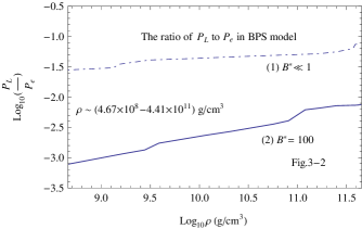
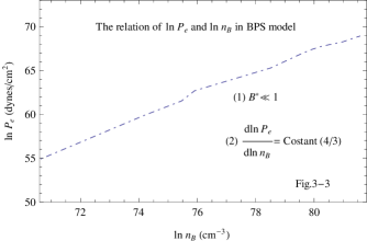
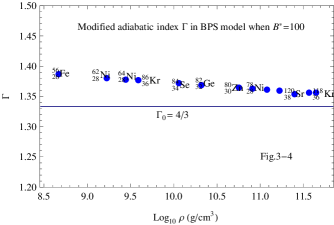
From the sub-diagram Fig.3-1, the matter pressure $P$ described by Eq.(24) increases obviously with density $\rho$ for both in a superhigh magnetic field and in the weak-field limit. Furthermore, given a density $\rho$, the value of $P$ in the case of the former ($B^{*}=100$)is bigger than that of $P$ in the case of the latter ($B^{*}\ll 1$), which can be easily seen from the curves of Fig.3-1. From the sub-diagram Fig.3-2, the ratios of $P_{L}$ to $P_{e}$ are about $10^{-2}$ and $10^{-3}$, respectively, corresponding to $B^{*}=100$ and $B^{*}\ll 1$, respectively. Therefore, one can infer that the contribution of $P_{L}$ to the matter pressure $P$ can be ignored if $B^{*}\geq 100$. In the sub-diagram Fig.3-3, we fit a curve of $\ln P_{e}$ versus $\ln n_{B}$ in the weak-field limit. Since the electrons are relativistic, the adiabatic index $\Gamma$ (i.e., the slope of the curve) is a constant of $4/3$, which is the standard relativistic value. In a strong magnetic field $B^{*}=100$, due to the changes of $P_{\rm e}$ and $\rho_{m}$, the values of modified $\Gamma$ are slightly higher than the constant of $4/3$, i.e, $\Gamma\equiv\ln P_{e}/\ln n_{B}\simeq 1.36\sim 1.39$, as illustrated in the sub-diagram Fig.3-4.

3.2 The QED effects on the EOS of BBP model

In the domain above neutron drip, as the matter density increases and the nuclei become more neutron rich, and the system becomes a mixture of nuclei, free neutrons, and electrons. When a critical value of baryon number density is reached, the nuclei disappear, essentially by merging together. Here we shall focus on the EOS of Baym, Bethe, and Pethick (1971) (see Ref.  BBP71)(hereinafter BBP), which describes such a system more successfully, compared with other models.

In this subsection, we’ll also assume an isotropic and homogenous matter pressure $P$ of this system, and will not discuss an anisotropy of the total pressure $P_{tot}$ of the system due to a strong magnetic field.

In the work by BBP, the major improvement was the introduction of a compressible liquid drop model of the nuclei (see Ref. BBP71). The energy density of BBP model is written as

$$\varepsilon=\varepsilon_{e}(n_{e})+n_{N}(W_{N}+W_{L})+n_{n}(1-~{}V_{N}n_{N})W_{n}~{}~{},~{}~{}$$ (25)

where $n_{n}$ is the number density of neutrons outside of nuclei (hereinafter neutron gas), and the new feature is the dependence on the volume of a nucleus $V_{N}$, which decreases with the outside pressure of the neutron gas. The baryon number density in this model is

$$n_{B}=An_{N}+(1-V_{N}n_{N})n_{n}~{}~{}~{},~{}~{}$$ (26)

where $V_{N}n_{N}$ and $1-V_{N}n_{N}$ are the fraction of volume occupied by nuclei, and the fraction occupied by the neutron gas, respectively. The matter pressure $p$ in BBP model is given by

$$P=P_{n}+P_{e}+P_{L}~{}~{}.~{}~{}$$ (27)

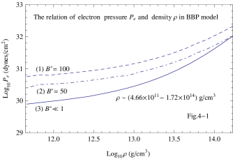
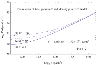
In the original work of BBP (1971), the three terms of $P_{n}$, $P_{e}$, $P_{L}$ in Eq.(27) are calculated by $P_{n}=n_{n}^{2}\frac{\partial E_{n}}{\partial n_{n}}$, $P_{e}=n_{e}^{2}\frac{\partial E_{e}}{\partial n_{e}}$, and $P_{L}=n_{N}^{2}\frac{\partial E_{L}}{\partial n_{N}}$, respectively. Ignoring the details of calculations, we list the values of chemical potentials $\mu_{e}$ and $\mu_{n}$ in Table 2, and cite the results of $P_{n}$, $P_{e}$ and $P$ in plotting Fig.4 from BBP (1971) and the review of Canuto (1974)(see Ref. Canuto74).

In a superhigh magnetic field, according to our model, the three pressure terms in Eq.(27) are approximately treated as follows: Sice the ratio of $P_{L}/P$ is $\sim 10^{-3}-10^{-4}$, the contribution of negative lattice pressure $P_{L}$ to the total dynamic pressure $P$ can be neglected; As in the magnetic BPS model, the electron pressure $P_{e}$ is also given by Eq.(21); In order to calculate the neutron pressure $P_{n}$, at first, ignoring the neutrino chemical potential $\mu_{\nu}$, we determine $\mu_{n}$ via $\beta$-equilibrium under a uniform superhigh magnetic field,

$$\mu_{e}+\mu_{p}+m_{p}c^{2}=\mu_{n}+m_{n}c^{2}~{}~{}~{},~{}~{}$$ (28)

where $\mu_{e}$ is the electron chemical potential, i.e., the electron Fermi energy $E_{\rm F}(e)$, including the rest-mass energy $m_{e}c^{2}$, $\mu_{p}$ is the proton chemical potential, i.e., the proton Fermi energy, not including the rest-mass energy $m_{p}c^{2}$ (notice that in BBP model the protons do not contribute the matter pressure because $\mu_{p}$ is negative), and $\mu_{n}$ is also called the neutron Fermi energy $E_{\rm F}^{{}^{\prime}}(n)$, not including its rest-mass energy $m_{n}c^{2}$, $\mu_{n}=E_{\rm F}^{{}^{\prime}}(n)=~{}\frac{p_{\rm F}^{2}(n)}{2m_{n}}$, secondly, by defining a non-dimensional variable $x_{n}=\frac{p_{\rm F}(n)}{m_{n}c}=\frac{\sqrt{2m_{n}\mu_{n}}}{m_{n}c}=\sqrt{\frac{2\mu_{n}}{m_{n}c^{2}}}$, we gain the polynomial $\phi(x_{n})$ of the variable $x_{n}$,

$$\phi(x_{n})=\frac{1}{8\pi^{2}}[x_{n}(1+x_{n}^{2})^{\frac{1}{2}}(\frac{2x_{n}^{2}}{3}-1)+ln[x_{n}+(1+x_{n}^{2})^{\frac{1}{2}}]]~{}~{},~{}~{}$$ (29)

where the neutrons are nonrelativistic (the density $\rho\ll 6\times 10^{15}$ g cm^-3 in BBP model), then $x_{e}\ll 1$, and $\phi(x_{n})\rightarrow\frac{1}{15\pi^{2}}(x_{n}^{5}-\frac{5}{14}x_{n}^{7}+\frac{5}{24}x_{n}^{9})$; finally, following Shapiro & Teukolsky (1983)(hereafter ST, see Ref. Shapiro83), we can calculate the value of $P_{n}$ by

$$P_{n}=\frac{m_{n}c^{2}}{\lambda_{n}^{3}}\phi(x_{n})~{}=1.624\times 10^{38}\frac{1}{15\pi^{2}}(x_{n}^{5}-\frac{5}{14}x_{n}^{7}+~{}\frac{5}{24}x_{n}^{9})~{}{\rm dynes~{}cm^{-2}}~{}~{},~{}~{}$$ (30)

where $\lambda_{n}~{}=~{}\frac{h}{m_{n}c}$ is the Compton wavelength of a neutron. In Table 2 we present the values of $\mu_{e}$ and $\mu_{n}$ corresponding to different magnetic fields in BBP model.

Values of $\mu_{e}$ and $\mu_{n}$ in magnetic BBP model. $\rho$ $A$ $Z$ $n_{N}\times 10^{-6}$ $n_{B}$ $Y_{e}^{{\dagger}}$ $\mu_{e}^{0}$ $\mu_{e}^{1}$ $\mu_{e}^{2}$ $\mu_{n}^{0}$ $\mu_{n}^{1}$ $\mu_{n}^{2}$ (g cm^-3) (fm^-3) (cm^-3) (MeV) (MeV) (MeV) (MeV) (MeV) (MeV) 4.66$\times 10^{11}$ 127 40 2.02 2.806$\times 10^{35}$ 0.2879 26.31 35.54 42.26 0.14 9.37 16.09 6.61$\times 10^{11}$ 130 40 2.13 3.981$\times 10^{35}$ 0.2315 26.98 36.72 43.67 0.37 10.11 17.06 8.79$\times 10^{11}$ 134 41 2.23 5.293$\times 10^{35}$ 0.1727 27.51 36.86 43.83 0.55 9.90 16.87 1.20$\times 10^{12}$ 137 42 2.34 7.226$\times 10^{35}$ 0.1360 28.13 37.32 44.38 0.75 9.94 17.10 1.47$\times 10^{12}$ 140 42 2.43 8.852$\times 10^{35}$ 0.1153 28.58 37.67 44.80 0.91 10.10 17.13 2.00$\times 10^{12}$ 144 43 2.58 1.204$\times 10^{36}$ 0.0921 29.33 38.47 45.74 1.15 10.29 17.56 2.67$\times 10^{12}$ 149 44 2.74 1.608$\times 10^{36}$ 0.0749 30.15 39.26 46.69 1.42 10.53 17.96 3.51$\times 10^{12}$ 154 45 2.93 2.114$\times 10^{36}$ 0.0624 31.05 40.17 47.76 1.71 10.83 18.42 4.54$\times 10^{12}$ 161 46 3.14 2.734$\times 10^{36}$ 0.0528 32.02 41.08 48.86 2.01 11.07 18.85 6.25$\times 10^{12}$ 170 48 3.45 3.764$\times 10^{36}$ 0.0439 33.43 42.52 50.56 2.45 11.54 19.58 8.38$\times 10^{12}$ 181 49 3.82 5.046$\times 10^{36}$ 0.0371 34.98 43.84 52.14 2.91 11.71 20.07 1.10$\times 10^{13}$ 193 51 4.23 6.624$\times 10^{36}$ 0.0326 36.68 45.44 54.03 3.41 12.17 20.76 1.50$\times 10^{13}$ 211 54 4.84 9.033$\times 10^{36}$ 0.0289 39.00 47.64 56.65 4.07 12.71 21.72 1.99$\times 10^{13}$ 232 57 5.54 1.198$\times 10^{37}$ 0.0264 41.56 49.99 59.45 4.77 13.20 22.66 2.58$\times 10^{13}$ 257 60 6.36 1.554$\times 10^{37}$ 0.0246 44.37 52.41 62.32 5.51 13.55 23.46 3.44$\times 10^{13}$ 296 65 7.52 2.071$\times 10^{37}$ 0.0236 48.10 55.73 66.28 6.47 14.10 24.65 4.68$\times 10^{13}$ 354 72 9.12 2.818$\times 10^{37}$ 0.0233 52.95 59.99 71.38 7.67 14.71 26.10 5.96$\times 10^{13}$ 421 78 10.7 3.589$\times 10^{37}$ 0.0235 57.56 64.38 76.56 8.77 15.90 27.77 8.01$\times 10^{13}$ 548 89 13.1 4.824$\times 10^{37}$ 0.0242 64.32 69.25 82.35 10.36 15.29 28.39 9.83$\times 10^{13}$ 683 100 15.0 5.920$\times 10^{37}$ 0.0253 69.81 73.76 87.72 11.66 15.61 29.57 1.30$\times 10^{14}$ 990 120 17.8 7.828$\times 10^{37}$ 0.0233 78.58 80.57 95.82 13.77 15.76 30.01 1.72${}^{{\ddagger}}\times 10^{14}$ 1640 157 19.6 1.035$\times 10^{38}$ 0.0297 88.84 88.28 104.98 16.39 15.83 32.53 2.00$\times 10^{14}$ 2500 210 18.8 1.205$\times 10^{38}$ 2.26$\times 10^{14}$ 4330 290 15.4 1.361$\times 10^{38}$ 2.39$\times 10^{14}$ 7840 445 11.0 1.439$\times 10^{38}$

In this Table, the signs of $`0^{\prime}$, $`1^{\prime}$ and $`2^{\prime}$ denote $B^{*}\ll 1$, $B^{*}=50$ and $B^{*}=100$, respectively, and the data of columns 1, 2, 3, 4, 7 and 10 are from Table 2 of Canuto (1974)(see Ref. Canuto74). The sign ‘${\dagger}$’ denotes the electron fraction $Y_{e}$ is given by $Y_{e}=Y_{p}=\frac{Zn_{N}}{n_{B}}\simeq\frac{Zn_{N}}{\rho/m_{u}}$, where $m_{u}=1.66057\times 10^{-24}$ g is the atom-mass unit because $n_{B}$ always can be treated as an invariable quantity in spit of a strong magnetic field. The sign ‘${\ddagger}$’denotes that the EOS of BBP model has been criticized by some authors (e.g., see Ref. Canuto74, Shapiro83), due to a monotonic and arbitrary increase of $Z$ with $A$, which causes the relation of $P$ and $\rho$ to be changed not much, so we stop listing the related calculations in the higher density region, $\rho\geq 1.72\times 10^{14}$ g cm^-3.

The values of $\mu_{n}$ are obtained from Eq.(28) ignoring the changes of kinetic energies and potential energies of protons in nuclei and the transformations between protons and neutrons caused by strong magnetic fields (i.e., keeping $\mu_{p}$ and $Y_{p}$ or $Y_{e}$ constant). In a superhigh magnetic field, the system under consideration is still a mixture of free neutrons, electrons, and nuclei. Since there is a lack of experimental data on the changes and transformations above, we still take the quantities $\mu_{p}$ and $Y_{p}$ as constants approximately when calculating $\mu_{e}$ and $\mu_{n}$. If $B\gg 10^{20}$ G, these ignorers are not permitted due to larger calculating errors. Note that such strong magnetic fields will no longer be taken into account according to our magnetar model (for details, see the following subsection). However, these ignorers can not affect our main result here that the values of $\mu_{e}$ and $\mu_{n}$ increase with increasing magnetic fields and densities. Based on Table 2 we plot four schematic sub-diagrams of QED effects on the EOS of BBP model, as shown in Fig.4.

(a)	(b)
(c)	(d)

Figure 4: The QED effects on the EOS of BBP model. Sub-diagrams Fig.4-1, Fig.4-2, Fig.4-3 and Fig.4-4 give $P_{e}$ versus $\rho$, $P$ versus $\rho$, $\Gamma$ versus $\rho$, and $\Delta\Gamma$ versus $\rho$, respectively, for this EOS in different magnetic fields. The matter pressure $P$ of this system is described by Eq.(27), assuming that $\mu_{p}$ and $Y_{e}$ are invariant approximately.

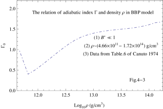
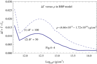
From sub-diagrams Fig.4-1 and Fig.4-2, both $P_{e}$ and $P$ obviously increase with density $\rho$ for the three cases. As in BPS model above, given a same density $\rho$, the stronger the magnetic field is, the higher the values of $P_{e}$ and $P$ become. However, the increments of $P_{e}$ and $P$ in the lower density region are larger than those in the higher density region. The main reason for this is that the increments of quantities $\mu_{e}$ and $\mu_{n}$ in the lower density region are larger than those in the higher density region, which can be easily seen in Table 2. In Fig.4-3 the curve of adiabatic index $\Gamma$ and $\rho$ in the weak-field limit is obtained by fitting with the data of Table 6 in Canuto (1974) (see Ref. Canuto74). The key feature of the curve in this sub-diagram is that $\Gamma$ decreases with increasing $\rho$ firstly, and then increases with increasing $\rho$. This phenomenon can be explained as follows: Firstly, as the neutron drip density $\rho_{d}$ is approached, the electrons are extremely relativistic, and the matter pressure is almost entirely due to electrons, therefore $\Gamma_{0}=4/3$; Secondly, slightly above $\rho_{d}$, the low-density neutron gas contributes appreciably to the density but not much to the matter pressure, and thus $\Gamma$ falls sharply. This drop in BBP model is described as $\Gamma=\frac{4}{3}[1-a(\rho-\rho_{d})^{1/2}]$, where $a$ is a positive constant. Thirdly, as the density increases (about $\rho\geq 10^{12}$ g cm^-3), the free neutrons nevertheless contribute to an increasingly larger fraction of the matter pressure. According to our calculations, in a strong magnetic field, e.g., $B^{*}\geq 50$, when $\rho\sim 10^{12}$ g cm^-3, $P_{\rm n}/P\sim 0.1-0.2$, while $\rho\sim 10^{13}-10^{14}$ g cm^-3, then $P_{n}/P\sim 0.8-0.99$, assuming that $\rho_{d}$ is unchanged. In addition, $\Gamma$ grows with increasing $B$ and $\rho$ slightly ($\Delta\Gamma\sim 10^{-2}-10^{-3}$) due to an increase in $P$, as shown in Fig.4-4.

3.3 The QED effects on the EOS of ideal $npe$ gas

In this subsection, we consider a homogenous ideal $npe$ gas under $\beta$- equilibrium, and adopt ST approximation corresponding to the weak-field limit (see Ref. Shapiro83) as the main method to treat EOS of this system in the density range of $0.5\rho_{0}\sim 2\rho_{0}$ where electrons are relativistic, neutrons and protons are non-relativistic. According to ST, when $\rho\gg 10^{13}$ g cm^-3, neutrons dominate in the interior of a NS, $\rho\approx m_{n}n_{n}$, then $n_{n}=1.7\times 10^{38}(\frac{\rho}{\rho_{0}})$ cm^-3 (see Ref. Shapiro83); employing $\beta$- equilibrium and charge neutrality gives $n_{p}=n_{e}=9.6\times 10^{35}(\frac{\rho}{\rho_{0}})^{2}$ cm^-3; $\beta$-equilibrium implies energy conservation and momentum conservation ($p_{\rm F}(p)=p_{\rm F}(e)$), we get $E_{\rm F}(e)=\mu_{n}=E_{\rm F}^{{}^{\prime}}(n)=p_{\rm F}^{2}(n)/2m_{n}=60(\frac{\rho}{\rho_{0}})^{2/3}$ MeV, and $\mu_{p}=E_{\rm F}^{{}^{\prime}}(p)=p_{\rm F}^{2}(p)/2m_{p}=1.9(\frac{\rho}{\rho_{0}})^{4/3}$ MeV; the isotropic matter pressure $P$ is given by

$$P=P_{e}+P_{p}+P_{n}$$

$$=\frac{m_{e}c^{2}}{\lambda_{e}^{3}}\phi(x_{e})+\frac{m_{p}c^{2}}{\lambda_{p}^{3}}\phi(x_{p})+\frac{m_{n}c^{2}}{\lambda_{n}^{3}}\phi(x_{n})~{}~{},~{}~{}$$ (31)

where $x_{p}=~{}\frac{p_{\rm F}(p)}{m_{p}c}=\frac{\sqrt{2m_{p}\mu_{p}}}{m_{p}c}~{}=~{}\sqrt{\frac{2\mu_{p}}{m_{p}c^{2}}}$, the expression of $\phi(x_{p})$ is completely similar to that of $\phi(x_{\rm n})$ (see Eq.(29)).

Based on the above results, we gain the following useful formulae:

$$P_{p}=1.169\times 10^{30}(\frac{\rho}{\rho_{0}})^{\frac{10}{3}}~{}~{}{\rm dynes~{}cm^{-2}}~{}~{},$$

$$P_{e}=1.825\times 10^{31}(\frac{\rho}{\rho_{0}})^{\frac{8}{3}}~{}~{}{\rm dynes~{}cm^{-2}}~{}~{},$$

$$P_{n}=6.807\times 10^{33}(\frac{\rho}{\rho_{0}})^{\frac{5}{3}}~{}~{}{\rm dynes~{}cm^{-2}}~{}~{},$$

$$Y_{e}=\frac{n_{e}}{n_{p}+n_{n}}\simeq\frac{n_{e}}{n_{n}}=0.005647(\frac{\rho}{\rho_{0}})~{}~{}.~{}~{}$$ (32)

Be note that these formulae in Eq.(32) always hold approximately in an ideal $npe$ gas when $B^{*}\ll 1$ and $\rho\sim 0.5\rho_{0}-2\rho_{0}$.

Our methods to treat EOS of an ideal $npe$ gas (system) under $\beta$-equilibrium in superhigh magnetic fields are introduced as follows: Combining Eq.(7) with momentum conservation $p_{\rm F}(p)=p_{\rm F}(e)$ gives the chemical potential $\mu_{p}=E_{\rm F}^{{}^{\prime}}(p)=1.005(\frac{B}{B_{\rm cr}}\frac{\rho}{\rho_{0}}\frac{Y_{e}}{0.0535})^{\frac{1}{2}}$  MeV, and the non-dimensional variable $x_{p}=\sqrt{\frac{2\mu_{p}}{m_{p}c^{2}}}\simeq 4.626\times 10^{-2}(\frac{B}{B_{\rm cr}}\frac{\rho}{\rho_{0}}\frac{Y_{e}}{0.0535})^{\frac{1}{4}}$; From Eq.(28), we get the non-dimensional variable,

$$x_{n}=\sqrt{\frac{1}{m_{n}c^{2}}}(2\times(43.44(\frac{B}{B_{\rm cr}}\frac{\rho}{\rho_{0}}\frac{Y_{e}}{0.0535})^{1/4}~{}$$

$$-1.29+1.005(\frac{B}{B_{\rm cr}}\frac{\rho}{\rho_{0}}\frac{Y_{e}}{0.0535})^{1/2}))^{1/2}.~{}~{}~{}$$ (33)

Thus, re-solving Eq.(31) gives the expression for the isotropic matter pressure $P$,

$$P=\frac{m_{e}c^{2}}{\lambda_{e}^{3}}\phi(x_{e})+\frac{m_{p}c^{2}}{\lambda_{p}^{3}}\phi(x_{p})+\frac{m_{n}c^{2}}{\lambda_{n}^{3}}\phi(x_{n})$$

$$=6.266\times 10^{30}(\frac{\rho}{\rho_{0}}\frac{B}{B_{\rm cr}}\frac{Y_{e}}{0.0535})+2.324\times 10^{26}(\frac{\rho}{\rho_{0}}\frac{B}{B_{\rm cr}}\frac{Y_{e}}{0.0535})^{\frac{5}{4}}$$

$$+1.624\times 10^{38}\frac{1}{15\pi^{2}}(x_{n}^{5}-\frac{5}{14}x_{n}^{7}+\frac{5}{24}x_{n}^{9})~{}{\rm dyne~{}cm^{-2}}~{}~{},~{}~{}$$ (34)

where $x_{n}$ is determined by Eq.(33). The above equation always approximately hold in an ideal $npe$ gas when $B^{*}\gg 1$ and $\rho~{}\sim 0.5\rho_{0}-~{}2\rho_{0}$.

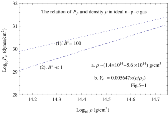
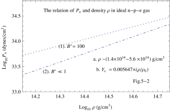
In order to calculate the matter pressure $P$ of an ideal $npe$ gas in a superhigh magnetic field, it’s better to an analytical expression for $Y_{p}$ (or $Y_{e}$) and $B$. Unfortunately, so far such an expression for $Y_{e}$ and $B$ has not been obtained yet. Furthermore, some related researches are unauthentic, due to the lack of observational supports. For example, Chakrabarty et al.(1997) studied the gross properties of cold symmetric matter, and matter in $\beta-$equilibrium under the influences of superhigh magnetic fields using a relativistic Hartree theory (see Ref. Chakrabarty97). Their main conclusions are as follows: Superhigh magnetic fields $\sim 10^{20}$ G could exist in the interior of a NS; $Y_{e}$ (or $Y_{p}$) is a strong function of $B$ and $\rho$; when an intense magnetic field is approached to the proton critical magnetic field, $B_{\rm cr}^{p}\sim 1.48\times 10^{20}$ G, the value of $Y_{p}$ (or $Y_{e}$) is expected to be enhanced considerably; by strongly modifying the phase spaces of protons (electrons), the field of $B\sim 10^{20}$ G can bring on a substantial $n\rightarrow p$ conversion, and the system is hence transformed into highly proton-rich matter with distinctively softer EOS (see Ref. Chakrabarty97). However, up to date, there have been no observations indicating the existence of fields $B\geq 10^{17}$ G inside a NS as mentioned in Section 1 of this paper. To sum up, magnetic fields of such magnitude ($\sim 10^{20}$ G) inside NSs are unauthentic, and are not consistent with our magnetar model (see Ref. Peng07, Ref. Gao11a, Ref.  Gao11b). In this letter, we assume the maximum magnetic field of a magnetar, $B\sim(3-4)\times 10^{15}$ G, in which $n_{B}$ always keeps invariable, and the changes of $n_{p}$ (or $n_{e}$) and $n_{n}$ caused by the equilibrium process of $e^{-}+p\leftrightarrow n+\nu$ are too small to be considered. Thus, the magnetic effects on the proton (or electron) fraction also can be ignored. In Table 3 we present the values of $E_{\rm F}(e)$, $\mu_{p}$, $\mu_{n}$ and $P$ in ideal $npe$ gas corresponding to two cases: $B^{*}\ll 1$ and $B^{*}=100$.

Values of $E_{\rm F}(e)$, $\mu_{p}$, $\mu_{n}$ and $P$ in ideal $n-p-e$ gas corresponding to $B^{*}\ll 1$ and $B^{*}=100$. $\rho$ $E_{\rm F}^{0}(e)$ $\mu_{p}^{0}$ $\mu_{n}^{0}$ $E_{\rm F}^{1}(e)$ $\mu_{\rm p}^{1}$ $\mu_{\rm n}^{1}$ $P^{0}$ $P^{1}$ (g cm^-3) (MeV) ( MeV) ( MeV ) ( MeV ) ( MeV ) ( MeV ) ( dynes cm^-2) ( dynes cm^-2) 1.4$\times 10^{14}$ 37.8 0.8 37.8 55.4 1.6 55.7 2.147$\times 10^{33}$ 5.247$\times 10^{33}$ 1.8$\times 10^{14}$ 44.7 1.1 44.7 62.8 2.1 63.6 3.265$\times 10^{33}$ 7.189$\times 10^{33}$ 2.0$\times 10^{14}$ 47.9 1.2 47.9 66.2 2.3 67.2 3.893$\times 10^{33}$ 8.204$\times 10^{33}$ 2.4$\times 10^{14}$ 54.1 1.5 54.1 72.5 2.8 74.0 5.278$\times 10^{33}$ 1.031$\times 10^{34}$ 2.8$\times 10^{14}$ 60.0 1.9 60.0 78.3 3.3 80.3 6.819$\times 10^{33}$ 1.251$\times 10^{34}$ 3.0$\times 10^{14}$ 62.8 2.1 62.8 81.0 3.5 83.2 7.659$\times 10^{33}$ 1.361$\times 10^{34}$ 3.4$\times 10^{14}$ 68.3 2.5 68.3 86.3 4.0 88.9 9.441$\times 10^{33}$ 1.595$\times 10^{34}$ 3.8$\times 10^{14}$ 73.5 2.9 73.5 91.2 4.4 94.4 1.136$\times 10^{34}$ 1.835$\times 10^{34}$ 4.2$\times 10^{14}$ 78.6 3.3 78.6 95.8 4.9 99.5 1.344$\times 10^{34}$ 2.081$\times 10^{34}$ 4.6$\times 10^{14}$ 83.5 3.7 83.5 100.4 5.4 104.4 1.564$\times 10^{34}$ 2.333$\times 10^{34}$ 5.0$\times 10^{14}$ 88.3 4.1 88.3 104.6 5.8 109.2 1.798$\times 10^{34}$ 2.591$\times 10^{34}$ 5.4$\times 10^{14}$ 93.0 4.6 93.0 108.7 6.3 113.7 2.045$\times 10^{34}$ 2.854$\times 10^{34}$ 5.6$\times 10^{14}$ 95.2 4.8 95.2 110.7 6.5 116.0 2.174$\times 10^{34}$ 2.987$\times 10^{34}$

The signs of ‘0’ and ‘1’ denote $B^{*}\ll 1$ and $B^{*}=100$, respectively. The values of $P^{0}$ and $P^{1}$ are obtained from Eq.(32) and Eq.(34), respectively. For simplicity, we ignore the change of $Y_{p}$ (or $Y_{e}$) caused by magnetic effects when calculating $P^{1}$. However, this assumption can not affect our main conclusion here that the dynamic pressure $P$ increases with increasing $B$ and $\rho$. Seeing from Table 3, for an ideal $npe$ system, the chemical potentials of fermions, as well as matter pressure, increases with increasing $B$ and $\rho$. Furthermore, the ratios of $P^{1}/P^{0}$ are in the range of $\sim 2.4~{}-1.4$ corresponding to a density range of ($1.4\times 10^{14}-~{}5.6\times 10^{14}$)g cm^-3, but the magnitudes of $P^{1}$ and $P^{0}$ are identical. Based on Table 3 we plot two schematic sub-diagrams of QED effects on EOS of this $npe$ gas, as shown in Fig.5.

(a)	(b)

Figure 5: The QED effects on $P_{p}$ and $P_{n}$ in ideal $npe$ gas. Sub-diagrams Fig.5-1 and Fig. 5-2 give $P_{p}$ versus $\rho$ and $P_{n}$ versus $\rho$, respectively, for an ideal $npe$ gas in a superhigh magnetic field. Here the ST approximation is adopted in treating EOS of this system under $\beta$-equilibrium in the weak-field limit.

From sub-diagrams Fig.5-1 and Fig.5-2, both $P_{p}$ and $P_{n}$ increase obviously with density $\rho$ and magnetic filed $B$. As in magnetic BPS and BBP models above, given a same density $\rho$, the values of $P_{p}$ and $P_{n}$ in a superhigh magnetic field (e.g.,$B^{*}~{}=100$) are higher than those in the weak-field limit.

As we know, in an ideal $npe$ system under strong magnetic fields, there is a positive correlation between the total matter energy density, $\epsilon$, and the total matter pressure, $P$,

$$P=-\frac{\partial\epsilon/n}{\partial\frac{1}{n}}=n^{2}\frac{\partial\epsilon/n}{\partial n}~{},~{}~{}~{}$$ (35)

where $n$ is equivalent to the number density of baryons, $P$ includes the electron pressure, $P_{e}$, proton pressure, $P_{p}$ and neutron pressure, $P_{n}$. Combining Eq.(34) with Eq.(35), we can conclude that the total matter energy density, $\epsilon$, increases with increasing $B$.

The stable configurations of a NS can be obtained from the well-known hydrostatic equilibrium equations of Tolman, Oppenheimer and Volkov (TOV) for the pressure $P(r)$ and the enclosed mass $m(r)$,

$$\frac{dP(r)}{dr}=-\frac{G(m(r)+4\pi r^{3}P(r)/c^{2})(\rho+P(r)/c^{2})}{r(r-2Gm(r)/c^{2})}$$

$$\frac{dm(r)}{dr}=4\pi\rho r^{2}~{},~{}~{}$$ (36)

where $G$ is the gravitational constant, see.Ref. Shapiro83. For a chosen central value of $\rho$, the numerical integration of Eq.(23) provides the mass-radius relation. However, we focus on a qualitative analysis of relation of $m(r)$ and $B$ in the context of a magnetar. In Eq.(36), the pressure $P(r)$ is the gravitational collapse pressure, and always be balanced by the total matter pressure, $P$; the central density $\rho$ is proportional to the matter energy density $\epsilon$; the enclosed mass, $m(r)$, increases with the central density $\rho$ when $r$ is given. From the calculations and analysis in this Section, we may expect a more massive stelar mass of a magnetars because the matter energy density, $\epsilon$, increases with $B$. Also, we propose that magnetars’ instability could be associated with the increased gravitational collapse pressure and high chemical potentials of fermions.

As we know, the magnetic effects can give rise to an anisotropy of the total pressure of the system to become anisotropic, e.g., see Ref. Bonazzola93, Bocquet95, Khalilov02,  Perez03, Perez08, Paulucci11. In an ideal $npe$ system, the total energy momentum tensor due to both matter and magnetic field is to be given by

$$T^{\mu\nu}=T^{\mu\nu}_{m}+T^{\mu\nu}_{B},~{},~{}~{}$$ (37)

where,

$$T^{\mu\nu}_{m}=\epsilon_{m}u^{\mu}u^{\nu}-P_{m}(g^{\mu\nu}-u^{\mu}u^{\nu})~{},~{}~{}$$ (38)

and

$$T^{\mu\nu}_{B}=\frac{B^{2}}{4\pi}(u^{\mu}u^{\nu}-\frac{1}{2}g^{\mu\nu})-\frac{B^{\mu}B^{\nu}}{4\pi}~{}.~{}~{}$$ (39)

where $\epsilon_{m}$ is the total matter energy density, and $P_{m}$ is the total matter pressure of the $npe$ system, respectively. The first term in Eq.(39) is equivalent to magnetic pressure, while the second term causes the magnetic tension. Assuming a uniform magnetic field $B$ directed along the $z$-axis, then we have

$$T^{\mu\nu}_{B}=\begin{bmatrix}\frac{B^{2}}{8\pi}&0&0&0\\ 0&\frac{B^{2}}{8\pi}&0&0\\ 0&0&\frac{B^{2}}{8\pi}&0\\ 0&0&0&-\frac{B^{2}}{8\pi}\end{bmatrix}.~{}~{}$$ (40)

Due to an excess negative pressure or tension along the direction to the magnetic field, the component of $T^{\mu\nu}_{B}$ along the field, $T^{zz}_{B}$, is negative. Thus, the total pressure in the parallel direction to the magnetic field can be written as

$$P_{\|}=P_{m}-\frac{B^{2}}{8\pi},~{}~{}$$ (41)

and that perpendicular to the magnetic field, $P_{\bot}$, is written as

$$P_{\bot}=P_{m}+\frac{B^{2}}{8\pi}~{}.~{}$$ (42)

From Eqs.(41-42), it’s obvious that the total pressure of the system becomes anisotropic. The parallel pressure $P_{\|}$ becomes negative, assuming that the magnetic pressure exceeds $P_{m}$. However, according to our calculations, when $B^{*}=100$, $P_{m}\sim 10^{33}-10^{34}$ dynes cm^-2 and $\frac{B^{2}}{8\pi}\sim 10^{29}-10^{30}$. Hence, in this presentation, we consider that the component of the total energy momentum tensor along the symmetry axis becomes positive, $T^{zz}>0$, since the total matter pressure increases more rapidly than the magnetic pressure. Accordingly, the total energy momentum tensor is given by

$$T^{\mu\nu}=\begin{bmatrix}\epsilon_{m}+\frac{B^{2}}{8\pi}&0&0&0\\ 0&P_{m}+\frac{B^{2}}{8\pi}&0&0\\ 0&0&P_{m}+\frac{B^{2}}{8\pi}&0\\ 0&0&0&(P_{m}+\frac{B^{2}}{8\pi})-\frac{B^{2}}{4\pi}\end{bmatrix}.~{}$$ (43)

A strong magnetic field can uncover anisotropy, see Ref. Perez03,  Perez08, due to magnetization pressure, ${\cal M}B$, where ${\cal M}$ is the magnetization of the system, which is given by

$${\cal M}=-\frac{\partial\epsilon_{m}}{\partial\textit{B}}.~{}$$ (44)

Therefore, the pressure perpendicular to the magnetic field, $P_{\bot}$, is actually written as

$$P_{\bot}=P_{m}+\frac{B^{2}}{8\pi}-\cal M\textit{B}.~{}$$ (45)

For a magnetic field $B\ll 10^{20}$ G, the magnetization is opposite to the external field $B$, i.e., ${\cal M}<0$, and it may happen that $P_{\bot}>P_{\|}$. For a magnetic field $B\geq 10^{20}$ G, the opposite occurs in some permeable materials where ${\cal M}>0$ and $P_{\bot}<P_{\|}$, this is due to ferromagnetic effects which have quantum origin, as in a gas of degenerate neutrons (see Ref.  Perez03, Perez08).

However, magnetars considered in the present work universally have typical surface dipole magnetic fields $\sim(10^{14}-10^{15})$ G and inner field strengths not more than $10^{17}$ G, under which $B^{2}/8\pi\gg\cal M\textit{B}$, and the effects of AMMs of nucleons on the EOS are ignored. Therefore, we exclude magnetization term in the total pressure. In other words, the exclusion of magnetization term cannot affect the result practically for the present purpose. Our model of magnetized ideal $npe$ gas favors the following relation: $P_{\bot}>P_{\|}$, which could lead to the Earth-like oblatening effect.

In the work of Bocquet et al.(see Ref Bocquet95), the authors considered an extension of the electromagnetic code developed by Bonazzola et al. (see Ref. Bonazzola93), and simulated high-magnetized rotating NSs. According to their simulations, the component of the total energy momentum tensor along the symmetry axis is negative, and the combined fluid-magnetic medium can develop a magnetic tension. As a result of this tension, the star displays a pinch across the symmetry axis and assumes a flattened shape (see Ref. Bocquet95).

Contrary to the work of Bocquet et al.(1995), we propose that the component of the total energy momentum tensor along the symmetry axis becomes positive, since the total matter pressure always grows more rapidly than the magnetic pressure. However, a similar effect is expected to occur in our present work, where the magnetic tension along the direction to the magnetic field will be responsible for deforming a magnetar along the magnetic field, and turns the star into a kind of oblate spheroid. Be note that such a deformation in shape might even render a more compact magnetar endowed with canonical strong surface fields $B\sim 10^{14-15}$ G. Also, such a deformed magnetar could have a more massive mass because of the positive contribution of the magnetic field energy to the EOS of the system.

4 Two contrary views on the relationship between $P_{e}$ and $B$

As we know, the electron pressure,$P_{e}$, as well as the electron Fermi energy $E_{\rm F}(e)$, is generally believed to decrease with increasing magnetic field strength $B$ (e.g., Ref. Lai91, Lai01).

According to statistical physics, the microscopic state number in a 6-dimension phase-space element $dxdydzdp_{x}dp_{y}dp_{z}$ is $dxdydzdp_{x}dp_{y}dp_{z}/h^{3}$. In the Ref. Canuto68, the number of states occupied by completely degenerate relativistic electrons in an unit volume is calculated as follows:

$$N_{phase}=\sum_{p_{x}}\sum_{p_{y}}\sum_{p_{z}}=\frac{1}{h^{3}}\int_{-\infty}^{\infty}\int_{-\infty}^{\infty}\int_{-\infty}^{\infty}dp_{x}dp_{y}dp_{z}$$

$$=\frac{1}{h^{3}}\int_{0}^{p_{\rm F}}dp_{z}\int_{0}^{\infty}p_{\bot}dp_{\bot}\int_{0}^{2\pi}d\Phi=\frac{\pi p_{\rm F}}{h^{3}}\int_{0}^{\infty}dp_{\bot}^{2}~{}~{},$$ (46)

where $\Phi~{}=~{}tan^{-1}p_{y}/p_{x}$. Quantization requires $p_{\bot}^{2}\rightarrow m^{2}c^{4}\frac{B}{B_{\rm cr}}2n$, hence, $\int_{0}^{\infty}dp_{\bot}^{2}\rightarrow\sum_{n=0}^{\infty}\omega_{n}$, where $\omega_{n}$ is the degeneracy of the $n$-th Landau level of electrons in relativistic magnetic field, which can be estimated as

$$\omega_{n}=\frac{1}{h^{2}}\int_{0}^{2\pi}d\phi\int_{A<p_{\bot}^{2}<B}p_{\bot}dp_{\bot}$$

$$=\frac{2\pi}{h^{2}}\frac{(B-A)}{2}=\frac{1}{2\pi}(\frac{\hbar}{m_{e}c})^{-2}\frac{B}{B_{\rm cr}}~{}~{},$$ (47)

where $A=m^{2}c^{2}\frac{B}{B_{\rm cr}}2n$, and $B=m^{2}c^{2}\frac{B}{B_{\rm cr}}2(n+1)$ (see Ref. Canuto71)

Be note, the above calculation method was cited from Statistical Mechanics (1965)(see Ref. Kubo65). The classical textbook, Statistical Mechanics (2003)(see Ref. Pathria03), also gives the expression for the degeneracy of the $n$-th Landau level of electrons in a relativistic magnetic field,

$$\omega_{n}=\frac{1}{h^{2}}\int dp_{x}dp_{y}=\frac{1}{h^{2}}\pi p_{\bot}^{2}\mid_{n}^{n+1}$$

$$=\frac{4\pi m_{e}\mu_{e}B}{h^{2}}=\frac{1}{2\pi}(\frac{\hbar}{m_{e}c})^{-2}\frac{B}{B_{\rm cr}}~{}~{},$$ (48)

where $\mu_{e}^{{}^{\prime}}=\frac{e\hbar}{2m_{e}c}$ is the electron magnetic moment. In the momentum interval $\Delta p_{z}$ along the direction to the magnetic field, for a non-relativistic electron gas, the number of possible microstates is given by

$$\frac{{e}BS}{2\pi\hbar c}\frac{L_{z}}{2\pi\hbar}\Delta p_{z}=\frac{{\rm e}BV}{4\pi^{2}\hbar^{2}c}~{}~{}.~{}~{}$$ (49)

(see Ref. Landau65). For the convenience of calculation, we assume $S=~{}1$ cm² and $V=~{}1$ cm³, and consider the electron spin degeneracy $g_{n0}=2-\delta_{n0}$ (when $n=0$, $g_{00}=1$; when $n\geq 1$, $g_{n0}=2$). From Eq.(49), we get the expression for the degeneracy of the n-th Landau level of electrons in a non-relativistic magnetic field,

$$\omega_{n}=g_{n0}\frac{eB}{2\pi\hbar c}=g_{n0}\frac{4\pi m_{e}\mu_{e}B}{h^{2}}~{}~{},~{}$$ (50)

where the solution of the non-relativistic electron cyclotron motion, $\hbar\omega_{B}=2\mu_{\rm e}B$, is used. Confusingly, the expression for the degeneracy of the $n$-th Landau level of electrons in a relativistic magnetic field is completely in accordance with that for the corresponding non-relativistic case, if one compare Eq.(47)(or Eq.(48)) with Eq.(50). After careful consideration and analysis, we find that Eq.(47) (or Eq.(48)) is just the expression we are looking for, that leads to an incorrect viewpoint on the electron Fermi energy, as well as the electron pressure, prevailing in the world currently. In our opinion, the expression for $\omega_{n}$ in Eq.(47)(or Eq.(48)) is incorrect, because it’s against the viewpoint on the quantization of Landau levels. The essence of the above method (or the incorrect deduction) lies in the assumption that the torus located between the $n$-th Landau level and the $(n+1)$-th Landau level in momentum space is ascribed to the $(n+1)$-th Landau level. Such a factitious assumption is equivalent to allow a continuous momentum (or energy) of an electron moving in the direction perpendicular to the magnetic field, which is obviously contradictory to the quantization of Landau levels in the case of a strong magnetic fields. The concept of Landau level quantization clearly tells us that there is no any microscopic quantum state between $p_{\bot}(n)$ and$p_{\bot}(n+1)$. In a word, the main cause of the popular incorrect viewpoint on $E_{\rm F}(e)$ is due to a factitious assumption.

In order to depict the quantization of Landau levels truly and accurately, we must introduce the Dirac $\delta$-function $\delta(\frac{p_{\bot}}{m_{e}c}-~{}[2(n+\sigma+\frac{1}{2})B^{*}]^{\frac{1}{2}})$ (see Ref. Gao11a, Gao12a). As we know, the eigenvector wave function of the Schrödinger equation (or Dirac equation) can be expanded in an infinite series. In the process of deducing the expressions concerning the quantization of Landau levels, we should firstly give a $p_{z}$ that changes continuously along the direction to the magnetic field, then solve the relativistic Schrödinger equation (or Dirac equation), finally obtain the maximum Landau level number, $n_{max}$, by truncating the infinite series when the wave function is limited (see Ref. Landau65). Logically, give $p_{z}$ firstly, and then determine the maximum Landau level number $n_{max}$.

As an alternative way to depict the quantization of Landau Levels of electrons in strong magnetic fields, we rewrite Eq.(50) as

$$\omega_{n}=\frac{1}{h^{2}}g_{n0}\int_{0}^{2\pi}d\phi\int\delta(\frac{p_{\bot}}{m_{e}c}-[2(n+\sigma+\frac{1}{2})B^{*}]^{\frac{1}{2}})p_{\bot}dp_{\bot}$$

$$=\frac{2\pi}{h^{2}}g_{n0}\int\delta(\frac{p_{\bot}}{m_{e}c}-~{}[2(n+\sigma+\frac{1}{2})B^{*}]^{\frac{1}{2}})p_{\bot}dp_{\bot}~{}~{},~{}$$ (51)

where $\phi=\arctan p_{y}/p_{x}$, and $g_{n0}=2-\delta_{n0}$ (when $n=0$, $g_{00}=1$; when $n\geq 1$, $g_{n0}=2$)is the electron spin degeneracy. In the interior of a NS, in the light of the Pauli exclusion principle, the electron number density should be equal to its microscopic state density,

$$N_{phase}=n_{e}=2\pi\frac{(m_{e}c)^{3}}{h^{3}}\int_{0}^{\frac{E_{\rm F}(e)}{m_{e}c^{2}}}d(\frac{p_{z}}{m_{e}c})\sum_{n=0}^{n_{max}(p_{z},\sigma,B^{*})}\sum g_{n0}$$

$$\int_{0}^{\frac{E_{\rm F}(e)}{m_{e}c^{2}}}\delta(\frac{p_{\bot}}{m_{e}c}-[2(n+\sigma+\frac{1}{2})B^{*}]^{\frac{1}{2}})\frac{p_{\bot}}{m_{e}c}d(\frac{p_{\bot}}{m_{e}c})=N_{A}\rho Y_{e}~{}~{}.~{}$$ (52)

In a word, when calculating $\omega_{n}$ and $N_{phase}$, we must take into account the Dirac $\delta$-function, otherwise, we would reach the wrong conclusion that $E_{\rm F}(e)$ decreases with the increase in $B$. Be note, in this letter, we first time propose that the electron pressure $P_{e}$ increases with increasing $B$, and the popular point of view on $P_{e}$ will be confronted with a severe challenge from our calculations

5 Summary Conclusions

In this paper we have derived a general expression for pressure of degenerate and relativistic electrons, which holds approximately when $B\gg B_{cr}$. We conclude that the stronger the magnetic field is, the higher the electron pressure becomes. The high electron pressure could be caused by the electron Fermi energy, which increases with the increase in the magnetic field strength. Given these arguments, the popular point of view on $P_{e}$ will be confronted with a severe challenge from our calculations.

Also, we have taken into account QED effects on EOSs of $BPS$ model, $BBP$ model and ideal $npe$ gas model, and have discussed an anisotropy of the total pressure of ideal $npe$ gas due to strong magnetic fields. Magnetars we have adopted in this work have typical surface dipole fields $B_{dip}\sim(10^{14}-10^{15})$ G, under which the effects of AMMs of nucleons on the total energy density and the total pressure have not been considered. The main conclusions are as follows: The total matter pressure $P$ increases with magnetic field strength $B$, because chemical potentials of fermions increase with increasing $B$, given a matter density $\rho$; taking into account of QED effects on the EOS, the total pressure is anisotropic; comparing with a common radio pulsar, a magnetar could be a more compact oblate spheroid-like deformed NS, due to the anisotropic total pressure; an increase in the maximum mass of a magnetar is expected because of the positive contribution of the magnetic field energy to the EOS.

Finally, it is earnestly hoped that our calculations can soon be combined with the latest studies and observations of magnetars, to present a deeper understanding of the nature of superhigh magnetic fields and bursts of magnetars.

References

- [1] C. Thompson and R. C. Duncan,Astrophys. J. 473, 322 (1996).
- [2] R. X. Xu, Astrophys. J. Lett. 570, 65 (2002).
- [3] R. X. Xu, Mon. Not. R. Astron. Soc. 356, 359 (2005).
- [4] Y. J. Du, G. J. Qiao, R. X. Xu and J. L. Han, Mon. Not. R. Astron. Soc. 399, 1587 (2009).
- [5] Q. H. Peng and H. Tong, Mon. Not. R. Astron. Soc. 378, 159 (2007).
- [6] Q. H. Peng and H. Tong, Proceedings of the Symposium on Nuclei in the Cosmos Mackinac Island, Michigan, USA, 27 July C1 August 2008 POS (NIC X) 189, (2009), [astro-ph.HE/0911.2066v1].
- [7] S. L. Shapiro and S. A. Teukolsky, Black Holes, White Drarfs, and Neutron Stars, New York, Wiley-Interscience, (1983).
- [8] D. G. Yakovlev, A. D. Kaminker, O. Y. Gnedin and P. Haensel, Phys. Rep. 354, 1 (2001).
- [9] D. Lai and S. L. Shapiro, Astrophys. J. 383, 745 (1991).
- [10] Z. F. Gao, N. Wang, D. L. Song, J. P. Yuan and C.-K. Chou, Astrophys. Space Sci. 334, 281 (2011).
- [11] Z. F. Gao, Q. H. Peng, N. Wang and C.-K. Chou, Astrophys. Space Sci. 342, 55 (2012).
- [12] V. Canuto and J. Ventura, Fund. Cosmic Phys., 2, 203 (1977).
- [13] Z. F. Gao, Q. H. Peng, N. Wang, C.-K. Chou and W. S. Huo Astrophys. Space Sci. 336, 427 (2011).
- [14] J. Ventura, W. Nagel and P. Mszros, Astrophys. J. Lett. 233, 125 (1979).
- [15] Z. F. Gao, Q. H. Peng, N. Wang and C.-K. Chou, Chinese Physics B 21(5), 057109(2012).
- [16] T. Bulik and M. C. Miller, Mon. Not. R. Astron. Soc. 288, 596 (1997).
- [17] K. Kohri and S. Yamada, Phy. Rev. D. 65, 043006 (2002), [astro-ph/0102225].
- [18] Wynn C. G. Ho and D. Lai, Mon. Not. R. Astron. Soc. 338, 233 (2003).
- [19] L. Kuiper, W. Hermsen and M. Mende, Astrophys. J. 613 , 1173 (2004).
- [20] S. Molkov, K. Hurley, R. Sunyaev, P. Shtykovsky, M. Revnivtsev and C. Kouveliotou, Astron. Astrophys.433, L13 (2005).
- [21] S. Mereghetti, D. Gtz, I. F. Mirabel and K. Hurley, Astron. Astrophys. 433 , L9 (2005).
- [22] She-Sheng. Xue, Phys. Rev. D. 68(1), 013004(2003).
- [23] A. Dupays, C. Rizzo, D. Bakalov and G. F. Bignami, Europhysics Letters. 82, 69002 (2008).
- [24] D. Mazur and J. S. Heyl, Mon. Not. R. Astron. Soc.412, 1381 (2011).
- [25] R. Battesti and C. Rizzo, Rep. Prog. Phys. 76, 016401 (2013).
- [26] D. Götz, S. Mereghetti, A. Tiengo and P. Esposito, Astron. Astrophys. 449 , L31(2006).
- [27] L. Kuiper, W. Hermsen, P. R. den Hartog and W. Collmar, Astrophys. J.645 , 556 (2006).
- [28] P. R. den Hartog, L. Kuiper and W. Hermsen, Astron. Astrophys.489, 263 (2008).
- [29] M. Lyutikov and F. P. Gavriil, Mon. Not. R. Astron. Soc.368, 690 (2006), [astro-ph/0507557].
- [30] M. G. Baring and A. K. Harding, Astrophys. Space Sci. 308 , 109 (2007).
- [31] N. Rea, S. Zane, R. Turolla, M. Lyutikov and D. Gtz, Astrophys. J.686 , 1245 (2008).
- [32] L. Nobili, R. Turolla and S. Zane, Mon. Not. R. Astron. Soc.389 , 989 (2008).
- [33] M. G. Baring, Z. Wadiasingh and P. L. Gonthier, Astrophys. J.733 , 61 (2011).
- [34] P. L. Gonthier, M. T. Eiles, Z. Wadiasingh, and M. G. Baring, Astronomical Society of the Pacific Conference Series, eds. W. Lewandowski, O, Maron and J. Kijak, Electromagnetic Radiation from Pulsars and Magnetars.466, 251 (2012)
- [35] E. E. Salpeter, Astrophys. J. 134, 669 (1961).
- [36] G. Baym, C. Pethick and P. Sutherland, Astrophys. J. 170, 299 (1971).
- [37] I. Fushiki, E. H. Gudmundsson and C. J. Pethick, Astrophys. J. 342, 958 (1989).
- [38] P. Haensel, J. L. Zdnik and J. Dobaczewski, Astron. Astrophys. 222, 353 (1989).
- [39] A. H. Wapstra and K. Bos, Atomic Data Nucl. Data Tables. 19 , 175 (1977).
- [40] A. H. Wapstra and K. Bos, Atomic Data Nucl. Data Tables. 17 , 474 (1976).
- [41] G. Baym, H. A. Bethe and C. J. Pethick, Nuclear Phys. A. 175, 225 (1971).
- [42] V. Canuto, Ann. Rev. Astron. Astrophys. 12, 167 (1974).
- [43] S. Chakrabarty, D. Bandyopadhyay, and S. Pal, Phy. Rev. Lett. 78, 75 (1997).
- [44] S. Bonazzola, E. Gourgoulhon, M. Salgado and J. A. Marck, Astron. Astrophys. 278, 421 (1993).
- [45] M. Bocquet, S. Bonazzola, E. Gourgoulhon and J. Novak, Astron. Astrophys. 301, 757 (1995).
- [46] V.R. Khalilov,Phys. Rev. D . 65(5), 056001 (2002).
- [47] A. Pérez Martínez, H. Pérez. Rojas and H. J. Mosqura Cuesta, Eur. Phys. J. C 29,111 (2003),[astro-ph/0303213].
- [48] A. Pérez Martínez, H. Pérez. Rojas and H. J. Mosqura Cuesta, Int.J. Mod. Phys. D.17, 210 (2008).
- [49] L. Paulucci, E. J. Ferrer, V. de La Incera and J. E. Horvath,Phys. Rev. D. 83(4), 043009 (2011).
- [50] D. Lai, Reviews of Modern Physics, 73, 629 (2001).
- [51] V. Canuto and H.Y. Chiu, Phys. Rev. 173, 1210 (1968).
- [52] V. Canuto and H.Y. Chiu, Space Sci. Rev., 12, 3 (1971).
- [53] R. Kubo, Statistics Mechanics , (Amsterdam: North-Holland Publishing Co. 1965), pp. 278–280.
- [54] R. K. Pathria, Statistics Mechanics, 2nd, (Singapore: Isevier. 2003), p. 280.
- [55] L. D. Landau and E. M.Lifshitz, Quantum Mechanics, ed. W. H. Freeman, (Pergamon Press, New York, 1965), pp. 459-460.