ON THE LIMIT OF EXTREME EIGENVALUES OF LARGE DIMENSIONAL RANDOM QUATERNION MATRICES

Abstract.

Since E.P.Wigner (1958) established his famous semicircle law, lots of attention has been paid by physicists, probabilists and statisticians to study the asymptotic properties of the largest eigenvalues for random matrices. Bai and Yin (1988) obtained the necessary and sufficient conditions for the strong convergence of the extreme eigenvalues of a Wigner matrix. In this paper, we consider the case of quaternion self-dual Hermitian matrices. We prove the necessary and sufficient conditions for the strong convergence of extreme eigenvalues of quaternion self-dual Hermitian matrices corresponding to the Wigner case.

1. Introduction

In nuclear physics, the energy levels are described by the eigenvalues of the Hamiltonian $\mathbf{H}_{n}$, which is regarded as an Hermitian matrix of very large order $n$. In the absence of any precise knowledge of $\mathbf{H}_{n}$, one assumes a reasonable probability distribution for its elements, from which we can deduce statistical properties of its spectrum. In history, the idea of a statistical mechanics of nuclei based on an ensemble of systems is due to Wigner [21, 18, 19], and is further developed by Dyson [8], Gaudin and Mehta [13]. Those foundational works can be viewed as the cornerstone of building-up the random matrix theory (RMT). The definition of random matrix ensembles consists of two parts [10]: the algebraic structure of the matrices $\mathbf{H}_{n}$ and the probability distributions of $\mathbf{H}_{n}$. In accordance to the consequences of time-reversal invariance, three kinds of ensembles were proposed: Gaussian orthogonal ensemble (GOE), Gaussian unitary ensemble (GUE), and Gaussian symplectic ensemble (GSE) (See [13] for details of those models ). In algebraic structure, the matrices $\mathbf{H}_{n}$ will be $n\times n$ real symmetric matrix, $n\times n$ complex Hermitian matrix and $n\times n$ quaternion self-dual Hermitian matrix, respectively. In the past several decades, Wigner’s program has drawn considerable attention from a large number of researchers and a huge body of literatures is aiming to get better understanding on those models. Preparing for what follows in this paper, it is necessary here to provide a short introduction to the quaternion self-dual Hermitian matrix since its structure is not as clear as the first two classes.

Quaternions were invented in 1843 by the Irish mathematician William Rowen Hamilton after a lengthy struggle to extend the theory of complex numbers to three dimensions [11, 6], and it is well known that the quaternion field $\mathbb{Q}$ can be represented as a two-dimensional complex vector space [4]. Thus this representation associates any $n\times n$ quaternion matrix with a $2n\times 2n$ complex matrix. Note that in this paper, we only use the $2n\times 2n$ complex representation of the quaternion matrices. Define four $2\times 2$ matrices:

$$\mathbf{e}=\left(\begin{array}[]{cc}1&0\\ 0&1\\ \end{array}\right),\quad\mathbf{i}=\left(\begin{array}[]{cc}i&0\\ 0&-i\\ \end{array}\right),\quad\mathbf{j}=\left(\begin{array}[]{cc}0&1\\ -1&0\\ \end{array}\right),\quad\mathbf{k}=\left(\begin{array}[]{cc}0&i\\ i&0\\ \end{array}\right)$$

where $i=\sqrt{-1}$. We can verify that:

$$\mathbf{i}^{2}=\mathbf{j}^{2}=\mathbf{k}^{2}=-\mathbf{e},\quad\mathbf{i}=\mathbf{j}\mathbf{k}=-\mathbf{k}\mathbf{j},$$

$$\mathbf{j}=\mathbf{i}\mathbf{k}=-\mathbf{k}\mathbf{i},\quad\mathbf{k}=\mathbf{i}\mathbf{j}=-\mathbf{j}\mathbf{i}.$$

For any real numbers $a,b,c,d,$ let

$$q=a\mathbf{e}+b\mathbf{i}+c\mathbf{j}+d\mathbf{k}=\left(\begin{array}[]{cc}a+bi&c+di\\ -c+di&a-bi\\ \end{array}\right)=\left(\begin{array}[]{cc}\lambda&\omega\\ -\bar{\omega}&\bar{\lambda}\\ \end{array}\right),$$

then $q$ is a quaternion. The quaternion conjugate of $q$ is defined by

$$\bar{q}=a\mathbf{e}-b\mathbf{i}-c\mathbf{j}-d\mathbf{k}=\left(\begin{array}[]{cc}a-bi&-c-di\\ c-di&a+bi\\ \end{array}\right)=\left(\begin{array}[]{cc}\bar{\lambda}&-\omega\\ \bar{\omega}&\lambda\\ \end{array}\right),$$

and the quaternion norm of $q$ is defined by

$$\|q\|=\sqrt{{a^{2}}+{b^{2}}+{c^{2}}+{d^{2}}}=\sqrt{{{\left|\lambda\right|}^{2}}+{{\left|\omega\right|}^{2}}}.$$

Remark 1.1.

We note that when we use the $2\times 2$ complex representation of quaternion $q$, the quaternion conjugate is in fact the ordinary conjugate transpose and $\|q\|^{2}$ is equal to the determinant of $q$.

An $n\times n$ quaternion self-dual Hermitian matrix $\mathbf{H_{n}}=(x_{jk})$ is a matrix whose entries $x_{jk}\ (j,k=1,\cdots,n)$ are quaternions and satisfy $x_{jk}=\bar{x}_{kj}$. Using the $2n\times 2n$ complex representation of $\mathbf{H}_{n}$ and according to Remark 1.1, $\mathbf{H}_{n}$ is obviously a $2n\times 2n$ Hermitian matrix. Then, we represent the entries of $\mathbf{H}_{n}$ as

$$x_{jk}=\left({\begin{array}[]{*{20}{c}}a_{jk}+b_{jk}i&c_{jk}+d_{jk}i\\ -{c}_{jk}+{d}_{jk}i&{a}_{jk}-{b}_{jk}i\end{array}}\right)=\left({\begin{array}[]{*{20}{c}}\lambda_{jk}&\omega_{jk}\\ {-\overline{\omega}}_{jk}&{\overline{\lambda}}_{jk}\end{array}}\right),1\leq j<k\leq n,$$

and $x_{jj}=\left({\begin{array}[]{*{20}{c}}a_{jj}&0\\ 0&a_{jj}\end{array}}\right),$ where $a_{jk},b_{jk},c_{jk},d_{jk}\in\mathbb{R}\ {\rm and}\ 1\leq j,k\leq n.$ Thus we can study the eigenvalues in the ordinary sense [10].

Remark 1.2.

It is known (see [23]) that the multiplicities of all the eigenvalues (obviously they are all real) of $\mathbf{H}_{n}$ are even and at least 2.

In RMT, suppose an $n\times n$ matrix $\mathbf{W}_{n}$ is Hermitian and let real numbers $s_{1}\geq s_{2}\geq\cdots\geq s_{n}$ denote the eigenvalues, then the empirical spectral distribution (ESD) of $\mathbf{W}_{n}$ is defined as:

$${F^{\mathbf{W_{n}}}}(x)=\frac{1}{n}\sum\limits_{i=1}^{n}{I({s_{i}}\leq x)},$$

where ${I(\cdot})$ is the indicator function. It is well known that if the entries on and above the diagonal of $\mathbf{W}_{n}$ are independent random variables with zero-mean and variance $\sigma^{2}$, then ${F^{\frac{1}{\sqrt{n}}{\mathbf{W}_{n}}}}(x)$ converges almost surely (a.s.) to a non-random distribution $F$ with density function:

(1.1) $$f(x)=\frac{1}{2\pi\sigma^{2}}\sqrt{4\sigma^{2}-x^{2}},~{}~{}x\in[-2\sigma,2\sigma],$$

which is known as the semicircle law. The semicircle law plays a very important role in many fields. However, one can not get the description of the behavior of the largest and the smallest eigenvalues from this distribution function. Juhász [12] and Füredi and Komlós [9] firstly studied the asymptotic properties of the extreme eigenvalues for Wigner matrix. In 1988, Bai and Yin [2] got the necessary and sufficient conditions for the almost surely convergence of the extreme eigenvalues. Then in [16], Tracy and Widom derived the limiting distribution of the largest eigenvalue of GOE, GUE, and GSE. In [22], the semicircular law for quaternion self-dual Hermitian matrices was proved under the most general condition of finite second moment. More recent results can be found in [14, 15, 17, 5, 7] and references therein.

2. Main theorem

In this paper, we study the asymptotic properties of the extreme eigenvalues for quaternion self-dual Hermitian matrices without Gaussian assumption. We shall show that the extreme eigenvalues of a high dimensional quaternion self-dual Hermitian matrix remain in certain bounded intervals. The main theorem can be described as following.

Theorem 2.1.

Suppose ${\mathbf{H}_{n}}=(x_{jk})$, where $x_{jk}=a_{jk}\mathbf{e}+b_{jk}\mathbf{i}+c_{jk}\mathbf{j}+d_{jk}\mathbf{k}$ is a quaternion self-dual Hermitian matrix whose entries on and above the diagonal are iid quaternion random variables. Then the largest eigenvalue of ${\mathbf{Q}_{n}}=\frac{1}{\sqrt{n}}{\mathbf{H}_{n}}$ tends to $\xi$ almost surely if and only if the following conditions hold:

(2.1) $$\begin{split}({\rm i})\quad&{\rm E}\left\|x_{11}^{+}\right\|^{2}<\infty,\quad where\ x^{+}={\rm max}(x,0),\\ ({\rm ii})\quad&{\rm E}a_{12}\leq 0\quad and\quad{\rm E}b_{12}={\rm E}c_{12}={\rm E}d_{12}=0,\\ ({\rm iii})\quad&{\rm E}\left\|x_{12}-{\rm E}x_{12}\right\|^{2}=\sigma^{2},\mbox{ and }\xi=2\sigma,\\ ({\rm iv})\quad&{\rm E}\left\|x_{12}\right\|^{4}<\infty.\\ \end{split}$$

According to the symmetry of the largest and smallest eigenvalues of a Hermitian matrix, we can easily derive the necessary and sufficient conditions for the existence of the limit of the smallest eigenvalue of a quaternion self-dual Hermitian matrix. Then we have the following theorem.

Theorem 2.2.

Suppose ${\mathbf{H}_{n}}=(x_{jk})$, where $x_{jk}=a_{jk}\mathbf{e}+b_{jk}\mathbf{i}+c_{jk}\mathbf{j}+d_{jk}\mathbf{k}$ is a quaternion self-dual Hermitian matrix whose entries on and above the diagonal are iid quaternion random variables. Then the largest eigenvalue of ${\mathbf{Q}_{n}}=\frac{1}{\sqrt{n}}{\mathbf{H}_{n}}$ tend to $\xi_{1}$ and the smallest eigenvalue of ${\mathbf{Q}_{n}}$ tends to $\xi_{2}$ almost surely if and only if the following conditions hold:

(2.2) $$\begin{split}({\rm i})\quad&{\rm E}\left\|x_{11}\right\|^{2}={\rm E}(a_{11})^{2}<\infty,\\ ({\rm ii})\quad&{\rm E}a_{12}={\rm E}b_{12}={\rm E}c_{12}={\rm E}d_{12}=0,\\ ({\rm iii})\quad&{\rm E}\left\|x_{12}\right\|^{2}=\sigma^{2},\mbox{ and }\xi_{1}=2\sigma,\ \xi_{2}=-2\sigma,\\ ({\rm iv})\quad&{\rm E}\left\|x_{12}\right\|^{4}<\infty.\\ \end{split}$$

3. Sufficiency of Conditions of Theorem 2.1

Now we are in position to present the proof of the sufficiency of conditions in (2.1). Obviously, we can assume $\sigma=1$ without loss of generality. To begin with, we shall give some lemmas that will be used. We note that $s_{\max}(\mathbf{Q}_{n})$ and $s_{\min}(\mathbf{Q}_{n})$ denote the largest and the smallest eigenvalues of matrix $\mathbf{Q}_{n}$ respectively throughout this paper.

3.1. Some knowledge in graph theory

To begin with, we shall introduce some acknowledge of graph theory. A graph is a triple $(E,V,F)$, where $E$ is the set of edges, $V$ is the set of vertices and $F$ is a function, $F:E\mapsto V\times V$. If $F(e)=(v_{1},v_{2})$, the vertices $v_{1},v_{2}$ are called the ends of edge $e$, $v_{1}$ is the initial of $e$ and $v_{2}$ is terminal of $e$. If $v_{1}=v_{2}$, edge $e$ is called a loop. If two edges have the same set of ends, they are said to be coincident.

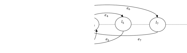
Let ${\mathbf{L}}=(l_{1},\cdots,l_{k})$ be a vector valued on $\{1,\cdots,n\}^{k}$. We define a $\Gamma$-graph as follows. Draw a horizontal line and plot the numbers $l_{1},\cdots,l_{k}$ on it. Consider the distinct numbers as vertices, and draw k edges $e_{j}$ from $l_{j}$ to $l_{j+1}$, $j=1,\cdots,k$, where $l_{k+1}=l_{1}$. Denote the number of distinct $l_{j}$’s by t. Such a graph is called a $\Gamma(k,t)$-graph. An example of $\Gamma$(8,5)-graph is shown in Figure 1.

Figure 1. A $\Gamma$-graph

Two $\Gamma(k,t)$-graphs are said to be isomorphic if one can be converted to the other by a permutation of $(1,\cdots,n)$. By the definition, all $\Gamma(k,t)$-graphs are classified into isomorphism classes.

A $\Gamma(k,t)$-graph is called canonical if it has the following properties:

1. It’s vertex set is $V=\{1,\cdots,t\}$.

2. It’s edge set is $E=\{e_{1},\cdots,e_{k}\}$.

3. There is a function $g$ from $\{1,\cdots,k\}$ onto $\{1,\cdots,t\}$ satisfying $g(1)=1$ and $g(l)\leq\max\{g(1),\cdots,g(l-1)\}+1$ for $1<l\leq k$.

4. $F(e_{l})=(g(l),g(l+1))$, for $l=1,\cdots,k$, with convention $g(k+1)=g(1)=1$.

It’s easy to see that each isomorphism class contains one and only one canonical $\Gamma(k,t)$-graph that is associated with a function $g$, and a general graph in this class can be defined by $F(e_{j})=(l_{g(j)},l_{g(j+1)})$. Therefore, we obtain each isomorphism class contains $n(n-1)\cdots(n-t+1)$ $\Gamma(k,t)$-graphs. The canonical $\Gamma(k,t)$-graphs can be classified into three categories:

Category 1 (denoted by $\Gamma_{1}(k,t)$):

A canonical $\Gamma(k,t)$-graph is said to belong to category 1 if each edge is coincident with exactly one other edge with opposite direction and the graph of noncoincident edges forms a tree (i.e., a connected graph without cycle). Obviously, there is no $\Gamma_{1}(k,t)$ if $k$ is odd. An example of $\Gamma_{1}$-graph is shown in Figure 2.

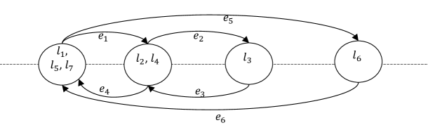
Figure 2. A $\Gamma_{1}$-graph

Category 2 ($\Gamma_{2}(k,t)$):

This category consists of all those canonical $\Gamma(k,t)$-graphs that have at least one single edge (an edge not coincident with any other edges). An example of $\Gamma_{2}$-graph is shown in Figure 3.

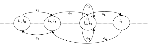
Figure 3. A $\Gamma_{2}$-graph

Category 3 ($\Gamma_{3}(k,t)$):

This category consists of all other canonical $\Gamma(k,t)$-graphs. Two examples of $\Gamma_{3}$-graph are shown in Figure 4 (one noncoincident edge has multiplicity 4) and Figure 5 (non-coincident edges form a cycle).

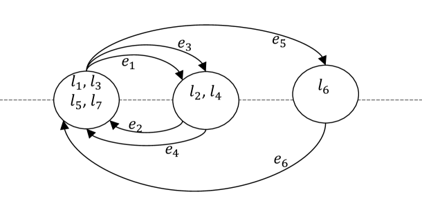
Figure 4. A $\Gamma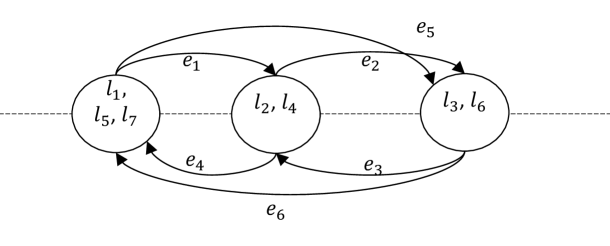_{3}$-graph

Figure 5. A $\Gamma_{3}$-graph

Obviously, in a $\Gamma_{3}(k,t)$-graph, we have $t\leq(k+1)/2$.

Now, classify the edges of a canonical $\Gamma(k,t)$-graph into several types:

1. If $g(a+1)={\rm max}(g(1),\cdots,g(a))+1$, the edge $e_{a}=(g(a),g(a+1))$ is called an innovation or a Type-1 $(T_{1})$ edge. A $T_{1}$ edge leads to a new vertex in the path $e_{1},\cdots,e_{a}$.

2. An edge is called a $T_{3}$ edge if it coincides with an innovation that is single until the $T_{3}$ edge appears. A $T_{3}$ edge $(g(a),g(a+1))$ is said to be irregular if there is only one innovation single up to $a$ (an edge $e$ is said to be single up to $a$ if it doesn’t coincide with any other edges in $\{(g(1),g(2)),\cdots,(g(a-1),g(a))\}$). All other $T_{3}$ edges are called regular $T_{3}$ edges.

3. All other edges are called $T_{4}$ edges.

4. The first appearance of a $T_{4}$ edge is called a $T_{2}$ edge. There are two cases: the first is the first appearance of a single noninnovation, and the second is that the first appearance of an edge that coincides with a $T_{3}$ edges.

Then, we shall give some lemmas without the proof.

Lemma 3.1 (Lemma 5.5 in [1]).

Let $t$ denote the number of $T_{2}$ edges and $l$ denote the number of innovations in $\{(g(1),g(2)),\cdots,(g(a-1),g(a))\}$ that are single up to $a$ and have a vertex coincident with $g(a)$. Then $l\leq t+1$.

Lemma 3.2 (Lemma 5.6 in [1]).

The number of regular $T_{3}$ edges is not greater than twice the number of $T_{2}$ edges.

3.2. Some auxiliary lemmas

Lemma 3.3.

If condition (i) of Theorem 2.1 holds, we have

$$\limsup\frac{1}{\sqrt{n}}\max_{k\leq n}a_{kk}^{+}=0.$$

Proof.

By Borel-Cantelli Lemma, it follows that

$${\rm E}(a_{11}^{+})^{2}<\infty\Rightarrow \sum_{n}{\rm P}\left((a_{11}^{+})^{2}>\varepsilon n\right)<\infty\Rightarrow\frac{(a_{nn}^{+})^{2}}{n}\to 0,\mbox{a.s.}$$

Thus, $\frac{1}{\sqrt{n}}\max\limits_{k\leq n}a_{kk}^{+}\to 0,\mbox{a.s.}$. ∎

Lemma 3.4.

Denote $\widetilde{\mathbf{Q}}_{n}=\frac{1}{\sqrt{n}}\left(\widetilde{x}_{jk}\right)$, where

$$\widetilde{x}_{jk}=\left\{\begin{array}[]{cc}\left(\begin{array}[]{cc}0&0\\ 0&0\\ \end{array}\right)&j=k\\ x_{jk}-{\rm E}x_{jk}&j\neq k\end{array}\right..$$

Then if the conditions (2.1) hold, then we have $\limsup s_{\max}\left(\mathbf{Q}_{n}\right)\leq\limsup s_{\max}(\widetilde{\mathbf{Q}}_{n})$.

Proof.

By condition (ii) and let $\mu={\rm E}a_{12}$, applying Lemma 3.3, one has

$$s_{\max}\left(\mathbf{Q}_{n}\right)=\max_{\left\|\mathbf{z}\right\|_{E}=1}\mathbf{z}^{*}\mathbf{Q}_{n}\mathbf{z}=\frac{1}{\sqrt{n}}\max_{\left\|\mathbf{z}\right\|_{E}=1}\left(\sum_{jk}z_{j}^{*}x_{jk}z_{k}\right)$$

$$= \max_{\left\|\mathbf{z}\right\|_{E}=1}\left[\frac{1}{\sqrt{n}}\sum_{j\neq k}z_{j}^{*}\left(x_{jk}-{\rm E}x_{jk}\right)z_{k}+\frac{\mu}{\sqrt{n}}\sum_{j,k}z_{j}^{*}z_{k}+\frac{1}{\sqrt{n}}\sum_{j}\left(a_{jj}-\mu\right)\left\|z_{j}\right\|_{E}^{2}\right]$$

$$\leq \max_{\left\|\mathbf{z}\right\|_{E}=1}\left[\frac{1}{\sqrt{n}}\sum_{j\neq k}z_{j}^{*}\left(x_{jk}-{\rm E}x_{jk}\right)z_{k}+\frac{1}{\sqrt{n}}\sum_{j}\left(a_{jj}^{+}-\mu\right)\left\|z_{j}\right\|_{E}^{2}\right]$$

$$\leq \max_{\left\|\mathbf{z}\right\|_{E}=1}\left[\frac{1}{\sqrt{n}}\sum_{j\neq k}z_{j}^{*}\left(x_{jk}-{\rm E}x_{jk}\right)z_{k}+\frac{1}{\sqrt{n}}\max_{j}\left(a_{jj}^{+}-\mu\right)\right]$$

$$\leq s_{\max}\left(\widetilde{\mathbf{Q}}_{n}\right)+o_{\rm a.s.}(1)$$

where  $\mathbf{z}=\left(z_{1}^{\prime},z_{2}^{\prime},\cdots,z_{n}^{\prime}\right)^{\prime},z_{j}$ is a $2\times 1$ vector for $j=1,\cdots,n$ and $\left\|\cdot\right\|_{E}$ denotes the Euclidean norm. ∎

Lemma 3.5.

If condition (iv) of Theorem 2.1 holds, we can select a sequence of constants  $\eta_{n}\downarrow 0$ satisfying

$${\rm P}(\mathbf{\widetilde{Q}_{n}}\neq\mathbf{\widehat{Q}_{n}},\ i.o.)=0,$$

where $\mathbf{\widehat{Q}_{n}}=\frac{1}{\sqrt{n}}\left(x_{jk}(1-\delta_{jk})I(\|x_{jk}\|\leq\eta_{n}\sqrt{n})\right)$, and $\delta_{jk}$ is the Kronecker delta. And the speed of $\eta_{n}\downarrow 0$ can be made arbitrarily slow.

Proof.

Note that Lemma 3.5 can be viewed as a generalization of Lemma 3.1 (Truncation Lemma) in [3], we shall omit the proof for brevity. ∎

By Lemma 3.5 and the fact that for any Hermitian matrices $A$ and $B$, $s_{\max}(A+B)\leq s_{\max}(A)+s_{\max}(B)$. Note that by the selection of $\eta_{n}$, we have $s_{\max}({\rm E}(\mathbf{\widehat{Q}_{n}}))\to 0$. We need only investigate the upper limit of $s_{\max}(\mathbf{\widehat{Q}_{n}}-{\rm E}(\mathbf{\widehat{Q}_{n}}))$. Combining Lemma 3.4 and Lemma 3.5, we shall prove the sufficiency of Theorem 2.1 under the following four assumptions:

$$\begin{split}({\rm i})\quad&x_{jj}=\left(\begin{array}[]{cc}0&0\\ 0&0\\ \end{array}\right).\\ ({\rm ii})\quad&{\rm E}a_{jk}={\rm E}b_{jk}={\rm E}c_{jk}={\rm E}d_{jk}=0,\sigma_{n}^{2}={\rm E}\left\|x_{jk}\right\|^{2}\leq 1\ {\rm for}\ j\neq k.\\ ({\rm iii})\quad&\left\|x_{jk}\right\|\leq\eta_{n}\sqrt{n}\ \ {\rm for}\ j\neq k.\\ ({\rm iv})\quad&{\rm E}\left\|x_{jk}^{l}\right\|\leq b\left(\eta_{n}\sqrt{n}\right)^{l-3}\ {\rm\ for\ some\ constant}\ b>0\ {\rm\ and\ all}\ j\neq k,l\geq 3.\end{split}$$

3.3. The proof of sufficiency of Theorem 2.1

Due to the Theorem 1.1 of [22], we have

$$\liminf_{n\to\infty}s_{\max}\left(\mathbf{Q}_{n}\right)\geq 2,{\rm a.s..}$$

Thus, it is sufficient to show that

$$\limsup_{n\to\infty}s_{\max}\left(\mathbf{Q}_{n}\right)\leq 2,{\rm a.s..}$$

For any even integer k and real number $\eta>2$, we have

(3.1) $${\rm P}\left(s_{\max}\left(\mathbf{Q}_{n}\right)\geq\eta\right)\leq{\rm P}\left({\rm tr}\left[\left(\mathbf{Q}_{n}\right)^{k}\right]\geq\eta^{k}\right)\leq\eta^{-k}{\rm E}\left({\rm tr}\left(\mathbf{Q}_{n}\right)^{k}\right).$$

To complete the proof, we shall select a sequence of $k_{n}=2m$ with the properties $k/\log\left(n\right)\to\infty$ and $k\eta_{n}^{1/3}/\log n\to 0$, and show that the right-hand side of (3.1) is summable. To this end, we will devote to estimate

$${\rm E}\left({\rm tr}\left(\mathbf{Q}_{n}\right)^{k}\right)= n^{-k/2}\sum_{j_{1},\cdots,j_{k}}{\rm Etr}\left(x_{j_{1}j_{2}}x_{j_{2}j_{3}}\cdots x_{j_{k}j_{1}}\right)$$

(3.2) $$= n^{-k/2}\sum_{G}\sum_{\mathbf{L}}{\rm Etr}\left(x_{G}(\mathbf{L})\right),$$

where the graphs G are  $\Gamma(k,t)$-graphs defined in Subsection 3.1. Note that if the graph G has a single edge, then the corresponding term is zero. So we only need to consider $\Gamma_{1}$ and $\Gamma_{3}$-graphs. Adopting the definition of types of edges in Subsection 3.1, (3.3) can be written as

(3.3) $${\rm E}\left({\rm tr}\left(\mathbf{Q}_{n}\right)^{k}\right)=n^{-k/2}{\sum}^{\prime}{\sum}^{\prime\prime}{\sum}^{\prime\prime\prime}{\rm Etr}\left(x_{j_{1}j_{2}}x_{j_{2}j_{3}}\cdots x_{j_{k}j_{1}}\right)$$

where ${\sum}^{\prime}$ is the summation for different arrangement of $T_{1},T_{3},T_{4}$-types edges, ${\sum}^{\prime\prime}$ is the summation for canonical graphs ($\Gamma_{1},\Gamma_{3}$) of the given arrangement of edges and ${\sum}^{\prime\prime\prime}$ is the summation for isomorphic graphs of the given canonical graph. Before estimating the righthand side of (3.3), we establish an inequality:

Lemma 3.6.

For $\forall\ j_{1},j_{2},\cdots,j_{k}$,

$$\left|{\rm tr}\left(x_{j_{1}j_{2}}x_{j_{2}j_{3}}\cdots x_{j_{k}j_{1}}\right)\right|\leq 2\left\|x_{j_{1}j_{2}}\right\|\left\|x_{j_{2}j_{3}}\right\|\cdots\left\|x_{j_{k}j_{1}}\right\|.$$

Proof.

Noticing that $x_{j_{1}j_{2}}x_{j_{2}j_{3}}\cdots x_{j_{k}j_{1}}$ can be written as $\left(\begin{array}[]{cc}\alpha&\beta\\ -\bar{\beta}&\bar{\alpha}\end{array}\right)$, and according to Remark 1.1, we have

$$\left|{\rm tr}\left(x_{j_{1}j_{2}}x_{j_{2}j_{3}}\cdots x_{j_{k}j_{1}}\right)\right|=\left|\alpha+\bar{\alpha}\right|\leq 2\left(\left|\alpha\right|^{2}+\left|\beta\right|^{2}\right)^{1/2}$$

$$= 2\left\{\det{\left(\begin{array}[]{cc}\alpha&\beta\\ -\bar{\beta}&\bar{\alpha}\end{array}\right)}\right\}^{1/2}$$

$$= 2\left\{\det\left(x_{j_{1}j_{2}}\right)\det\left(x_{j_{2}j_{3}}\right)\cdots\det\left(x_{j_{k}j_{1}}\right)\right\}^{1/2}$$

$$= 2\left\|x_{j_{1}j_{2}}\right\|\left\|x_{j_{2}j_{3}}\right\|\cdots\left\|x_{j_{k}j_{1}}\right\|.$$

∎

Applying Lemma 3.6 to (3.3), we have

(3.4) $${\rm E}\left({\rm tr}\left(\mathbf{Q}_{n}\right)^{k}\right)\leq 2n^{-k/2}{\sum}^{\prime}{\sum}^{\prime\prime}{\sum}^{\prime\prime\prime}{\rm E}\left\|x_{j_{1}j_{2}}\right\|\left\|x_{j_{2}j_{3}}\right\|\cdots\left\|x_{j_{k}j_{1}}\right\|.$$

For $\Gamma_{1}$ and $\Gamma_{3}$-graphs, suppose that there are $l\ (l\leq m)$ innovations and $t$ $T_{2}$ edges in the graph G. Then there are $l$ $T_{3}$ edges, $k-2l$ $T_{4}$ edges and $l+1$ noncoincident vertices. We obtain that ${\sum}^{\prime}\leq\sum_{l=1}^{k/2}{k\choose l}{k-l\choose l}$. By Lemmas 3.1 and 3.2, we know that ${\sum}^{\prime\prime}\leq\sum_{t=0}^{k-2l}\left(t+1\right)^{2(k-2l)}{k^{2}\choose t}\left(t+1\right)^{k-2l}$. Obviously, ${\sum}^{\prime\prime\prime}$ is bounded by $n^{l+1}$. Then, together with (3.4), we have

$${\rm E}\left({\rm tr}\left(\mathbf{Q}_{n}\right)^{k}\right)\leq 2n^{-k/2}\sum_{l=1}^{[k/2]}\sum_{t=0}^{k-2l}n^{l+1}\bigg{(}\begin{array}[]{cc}k\\ l\end{array}\bigg{)}\bigg{(}\begin{array}[]{cc}k-l\\ l\end{array}\bigg{)}\bigg{(}\begin{array}[]{cc}k^{2}\\ t\end{array}\bigg{)}\left(t+1\right)^{3(k-2l)}b^{t}\left(\sqrt{n}\eta_{n}\right)^{k-2l-t}$$

$$\leq 2n\sum_{l=1}^{[k/2]}\frac{k!}{l!l!(k-2l)!}\sum_{t=0}^{k-2l}k^{2t}\left(t+1\right)^{3(k-2l)}b^{t}\eta_{n}^{k-2l}\left(\sqrt{n}\eta_{n}\right)^{-t}$$

$$= 2n\sum_{l=1}^{[k/2]}\frac{k!}{l!l!(k-2l)!}\sum_{t=0}^{k-2l}\left(t+1\right)^{3(k-2l)}\left[\frac{bk^{2}}{\sqrt{n}\eta_{n}}\right]^{t+1}\eta_{n}^{k-2l}\frac{\sqrt{n}\eta_{n}}{bk^{2}}$$

$$= \frac{2\eta_{n}n^{3/2}}{bk^{2}}\sum_{l=1}^{[k/2]}\frac{k!}{l!l!(k-2l)!}\sum_{t=0}^{k-2l}\left(t+1\right)^{3(k-2l)}\left[\frac{bk^{2}}{\sqrt{n}\eta_{n}}\right]^{t+1}\eta_{n}^{k-2l}.$$

Due to the elementary inequality

$$\alpha^{-(t+1)}\left(t+1\right)^{\beta}\leq\left(\frac{\beta}{\log(\alpha)}\right)^{\beta}$$

where $\beta>0,\alpha>1$, for large $n$ we have

$${\rm E}\left({\rm tr}\left(\mathbf{Q}_{n}\right)^{k}\right)\leq \frac{2\eta_{n}n^{3/2}}{bk^{2}}\sum_{l=1}^{k/2}\frac{k!}{l!l!(k-2l)!}\sum_{t=0}^{k-2l}\eta_{n}^{k-2l}\left(\frac{3(k-2l)}{\log(\sqrt{n}\eta_{n}/bk^{2})}\right)^{3(k-2l)}$$

$$\leq 2n^{3/2}\sum_{l=1}^{k/2}\frac{k!}{l!l!(k-2l)!}\eta_{n}^{k-2l}\left(\frac{10k}{\log n}\right)^{3(k-2l)}$$

$$\leq 2n^{3/2}\left[1+1+\left(\frac{10k\eta_{n}^{1/3}}{\log n}\right)^{3}\right]^{k}$$

(3.5) $$= 2n^{3/2}\left[2+o(1)\right]^{k}$$

where the last inequality follows from $k\eta_{n}^{1/3}/\log n\to 0$ . Finally, together with (3.1) and (3.3), we have

$$\sum_{n}{\rm P}\left(s_{\max}\left(\mathbf{Q}_{n}\right)\geq\eta\right)\leq 2\sum_{n}\frac{n^{3/2}\left[2+o(1)\right]^{k}}{\eta^{k}}$$

$$\leq 2\sum_{n}n^{3/2}e^{k\log{\frac{2+o(1)}{\eta}}}$$

$$= \sum_{n}\left(2n\right)^{3/2+{\frac{k}{\log\left(2n\right)}\log{\frac{2+o(1)}{\eta}}}}<\infty$$

where the last inequality follows from the fact that $k/\log n\to\infty$. The sufficiency is proved.

4. Necessity of Conditions of Theorem 2.1

4.1. Necessity of condition (i)

Suppose that $\limsup s_{\max}\left(\mathbf{Q}_{n}\right)\leq\xi,{\rm a.s.}$. Then,

$$s_{\max}\left(\mathbf{Q}_{n}\right)= \max_{\left\|\mathbf{z}\right\|_{E}=1}\mathbf{z}^{*}\mathbf{Q}_{n}\mathbf{z}\geq\frac{1}{\sqrt{n}}\left(0,\cdots,0,1\right)\mathbf{Q}_{n}\left(0,\cdots,0,1\right)^{\prime}=\frac{a_{nn}}{\sqrt{n}}$$

which implies that $\frac{a_{nn}^{+}}{\sqrt{n}}\leq\max\left\{0,s_{\max}\left(\mathbf{Q}_{n}\right)\right\}.$
Applying Borel-Cantelli lemma, for any $\eta>\xi$, we have

$$\limsup\frac{a_{nn}^{+}}{\sqrt{n}}<\eta,{\rm a.s.}\Rightarrow{\rm P}\left(\frac{a_{nn}^{+}}{\sqrt{n}}\geq\eta,{\rm i.o.}\right)=0\Rightarrow\sum_{n=1}^{\infty}{\rm P}\left(a_{11}^{+}\geq\eta\sqrt{n}\right)<\infty,$$

which implies ${\rm E}(a_{11}^{+})^{2}<\infty$.

4.2. Necessity of condition (iv)

Assume that condition (i) holds. Let $\mathcal{N}_{l}=\left\{j;2^{l}<j\leq 2^{l+1};\left\|x_{jj}\right\|\leq 2^{l/4}\right\}$, $N_{l}={\#}\left(\mathcal{N}_{l}\right)$ and $p={\rm P}\left(\left\|x_{11}\right\|\leq 2^{l/4}\right)$. When $n\in(2^{l+1},2^{l+2}]$, for $x_{jk}\neq 0$ and $j,k\in\mathcal{N}_{l}$, construct a unit complex vector $\mathbf{z}$ by taking $z_{k}^{*}=\left(\frac{1}{\sqrt{2}},0\right),z_{j}^{*}=\left(\frac{\bar{\lambda}_{jk}}{\sqrt{2}\left\|x_{jk}\right\|},-\frac{\omega_{jk}}{\sqrt{2}\left\|x_{jk}\right\|}\right)$ and $z_{l}^{*}=\left(0,0\right)\left(l\neq j,l\neq k\right)$. Then, we obtain

$$s_{\max}(\mathbf{Q}_{n})\geq\mathbf{z^{*}Q_{n}z}=\frac{1}{\sqrt{n}}\sum_{j,k}{z_{j}^{*}}x_{jk}{z_{k}}=\frac{1}{\sqrt{n}}\left[\left\|x_{jk}\right\|+\frac{1}{2}\left(a_{jj}+{a_{kk}}\right)\right]$$

$$\Rightarrow s_{\max}({\mathbf{Q}}_{n})\geq 2^{-l/2-1}\max_{j,k\in\mathcal{N}_{l}}\left\{\left\|x_{jk}\right\|\right\}-2^{-l/4-1}.$$

Obviously, when $x_{jk}=\left(\begin{array}[]{cc}0&0\\ 0&0\\ \end{array}\right)$, the conclusion is still true. Moreover, we have known that for any $\eta>\xi$,

$${\rm P}\left(\max_{2^{l+1}<n\leq 2^{l+2}}s_{\max}\left(\mathbf{Q}_{n}\right)\geq\eta,{\rm i.o.}\right)=0.$$

Combining the above inequality and Borel-Cantelli lemma, it follows that

(4.1) $$\sum_{l=1}^{\infty}{\rm P}\left(\max_{j,k\in\mathcal{N}_{l}}\left\{\left\|x_{jk}\right\|\right\}\geq\eta 2^{l/2+1}\right)<\infty.$$

Noticing that $N_{l}$ and $x_{jk}$ are independent, we have

$${\rm P}\left(\max_{j,k\in\mathcal{N}_{l}}\left\{\left\|x_{jk}\right\|\right\}\geq\eta 2^{l/2+1}\bigg{|}N_{l}=r\right)$$

$$= {\rm P}\left(\max_{1\leq j<k\leq r}\left\{\left\|x_{jk}\right\|\right\}\geq\eta 2^{l/2+1}\right)$$

$$= 1-\left[1-{\rm P}\left(\left\|x_{12}\right\|\geq\eta 2^{l/2+1}\right)\right]^{r(r-1)/2}.$$

Denote $N_{l}\sim B\left(2^{l},p\right)$, therefore, one has

$${\rm P}\left(\max_{j,k\in\mathcal{N}_{l}}\left\{\left\|x_{jk}\right\|\right\}\geq\eta 2^{l/2+1}\right)$$

$$= \sum_{r=0}^{2^{l}}{\rm P}\left(N_{l}=r\right){\rm P}\left(\max_{j,k\in\mathcal{N}_{l}}\left\{\left\|x_{jk}\right\|\right\}\geq\eta 2^{l/2+1}\bigg{|}N_{l}=r\right)$$

(4.4) $$\geq \sum_{r=2^{l-1}+1}^{2^{l}}\left(\begin{array}[]{cc}2^{l}\\ r\end{array}\right)p^{r}\left(1-p\right)^{2^{l}-r}\left\{1-\left[1-{\rm P}\left(\left\|x_{12}\right\|\geq\eta 2^{l/2+1}\right)\right]^{r(r-1)/2}\right\}$$

(4.5) $$\geq \frac{1}{2}\left\{1-\left[1-{\rm P}\left(\left\|x_{12}\right\|\geq\eta 2^{l/2+1}\right)\right]^{2l-3}\right\}$$

where the last inequality follows from that $p$ is close to 1 for all large $l$. From (4.1) and (4.2), we acquire that

$$\sum_{l=1}^{\infty}\left\{1-\left[1-{\rm P}\left(\left\|x_{12}\right\|\geq\eta 2^{l/2+1}\right)\right]^{2l-3}\right\}<\infty$$

$$\Rightarrow \prod_{l=1}^{\infty}\left[1-{\rm P}\left(\left\|x_{12}\right\|\geq\eta 2^{l/2+1}\right)\right]^{2l-3}>0$$

$$\Rightarrow \sum_{l=1}^{\infty}2^{2l-3}{\rm P}\left(\left\|x_{12}\right\|\geq\eta 2^{l/2+1}\right)<\infty$$

$$\Rightarrow {\rm E}\left\|x_{12}\right\|^{4}<\infty.$$

4.3. Necessity of condition (ii)

Assume that conditions (i) and (iv) hold. Firstly, we will show that $a={\rm E}\left(a_{12}\right)\leq 0$. Suppose that $a>0$. Let $\mathcal{D}_{n}=\left\{j\leq n,\left\|x_{jj}\right\|<n^{1/4}\right\}$, $N=\#\left(\mathcal{D}_{n}\right)$ and $\widetilde{\mathbf{Q}}_{n}=\frac{1}{\sqrt{n}}\left(\widetilde{x}_{jk}\right)$ with $\widetilde{x}_{jk}=\left\{\begin{array}[]{cc}\left(\begin{array}[]{cc}0&0\\ 0&0\\ \end{array}\right)&j=k\\ x_{jk}&j\neq k\end{array}\right.$. Construct a unit vector $\mathbf{z}^{*}=\left(z_{1}^{*},\cdots,z_{n}^{*}\right)$ by taking $z_{j}^{*}=(\frac{1}{\sqrt{N}},0)\ {\rm if}\ j\in\mathcal{D}_{n}\ {\rm and}\ z_{j}^{*}=(0,0)\ {\rm otherwise}$, then we have

$$s_{\max}(\mathbf{Q}_{n})\geq \mathbf{z^{*}Q_{n}z}$$

$$= \mathbf{z^{*}(Q_{n}-\widetilde{Q}_{n})z}+\mathbf{z^{*}(\widetilde{Q}_{n}-{\rm E}\widetilde{Q}_{n})z}+\mathbf{z^{*}({\rm E}\widetilde{Q}_{n})z}$$

$$\geq \frac{1}{N\sqrt{n}}\sum_{j\in\mathcal{D}_{n}}a_{jj}+\mathbf{z^{*}(\widetilde{Q}_{n}-{\rm E}\widetilde{Q}_{n})z}+\frac{a(N-1)}{\sqrt{n}}$$

$$\geq -n^{-1/4}+s_{\min}\mathbf{(\widetilde{Q}_{n}-{\rm E}\widetilde{Q}_{n})}+\frac{a(N-1)}{\sqrt{n}}$$

$$\geq -n^{-1/4}-2\sigma+\frac{a(N-1)}{\sqrt{n}}\to\infty$$

which contradicts with the assumption that $\limsup s_{\max}\left(\mathbf{Q}_{n}\right)=2\sigma$ almost surely. Here, we have used a fact that $s_{\min}\mathbf{(\widetilde{Q}_{n}-{\rm E}\widetilde{Q}_{n})}\to-2\sigma$, a.s. which is an easy consequence of the sufficient part of the theorem.

Now, we proceed to show that ${\rm E}b_{12}={\rm E}c_{12}={\rm E}d_{12}=0$. To this end, we shall quote the following lemma:

Lemma 4.1 (Lemma 2.7 in [1]).

Let $\mathbf{A}_{n}$ be an $n\times n$ skew-symmetric matrix whose elements above the diagonal are 1 and those below the diagonal are -1. Then, the eigenvalues of $\mathbf{A}_{n}$ are $\lambda_{k}=-i\cot\left(\pi\left(2k-1\right)/2n\right),k=1,2,\cdots,n$. The eigenvector associated with $\lambda_{k}$ is $\mathbf{u}_{k}=\frac{1}{\sqrt{n}}\left(1,\rho_{k},\cdots,\rho_{k}^{n-1}\right)^{\prime}$, where $\rho_{k}=\left(\lambda_{k}-1\right)/\left(\lambda_{k}+1\right)=\exp\left(-i\pi\left(2k-1\right)/n\right)$.

Since we shall use matrix similarity transformation to get a similar matrix of $\mathbf{Q}_{n}$, written as:

$$\widetilde{\widetilde{\mathbf{Q}}}_{n}=\frac{1}{\sqrt{n}}\left(\begin{array}[]{cc}\Sigma_{1}&\Sigma_{2}\\ -\overline{\Sigma}_{2}&\overline{\Sigma}_{1}\end{array}\right),$$

where $\Sigma_{1}=\left(\lambda_{jk}\right)_{n\times n},\Sigma_{2}=\left(\omega_{jk}\right)_{n\times n}$, $\bar{\Sigma}_{1}=\left(\bar{\lambda}_{jk}\right)_{n\times n}$ while $\bar{\Sigma}_{2}=\left(\bar{\omega}_{jk}\right)_{n\times n}$. Of course, $\widetilde{\widetilde{\mathbf{Q}}}_{n}$ has the same eigenvalues as ${\mathbf{Q}}_{n}$. Let $\mathbf{A}_{n}$ be an $n\times n$ skew-symmetric matrix whose elements above the diagonal are 1 and those below the diagonal are -1 and let $\breve{\mathbf{Q}}_{n}$ be the matrix obtained from $\widetilde{\widetilde{\mathbf{Q}}}_{n}$ by replacing $\Sigma_{1},\Sigma_{2}$’s diagonal elements with zero. Let $\mathbf{J}$ be the $n\times n$ matrix of $1$’s and $\mathbf{I}$ be the $n\times n$ identity matrix. Suppose ${\rm E}b_{12}=b,{\rm E}c_{12}=c,{\rm E}d_{12}=d$, then write

$${\rm E}\breve{\mathbf{Q}}_{n}$$

$$= \frac{1}{\sqrt{n}}\left(a\left(\begin{array}[]{cc}\mathbf{J}-\mathbf{I}&0\\ 0&\mathbf{J}-\mathbf{I}\end{array}\right)+ib\left(\begin{array}[]{cc}\mathbf{A}_{n}&0\\ 0&-\mathbf{A}_{n}\end{array}\right)+c\left(\begin{array}[]{cc}0&\mathbf{A}_{n}\\ -\mathbf{A}_{n}&0\end{array}\right)+id\left(\begin{array}[]{cc}0&\mathbf{A}_{n}\\ \mathbf{A}_{n}&0\end{array}\right)\right)$$

$$= {\rm\mathbf{R}_{n}}+{\rm\mathbf{M}_{n}},$$

where

$${\rm\mathbf{R}_{n}}=\frac{a}{\sqrt{n}}\left(\begin{array}[]{cc}\mathbf{J}-\mathbf{I}&0\\ 0&\mathbf{J}-\mathbf{I}\end{array}\right)$$

$${\rm\mathbf{M}_{n}}=\frac{1}{\sqrt{n}}\left(ib\left(\begin{array}[]{cc}\mathbf{A}_{n}&0\\ 0&-\mathbf{A}_{n}\end{array}\right)+c\left(\begin{array}[]{cc}0&\mathbf{A}_{n}\\ -\mathbf{A}_{n}&0\end{array}\right)+id\left(\begin{array}[]{cc}0&\mathbf{A}_{n}\\ \mathbf{A}_{n}&0\end{array}\right)\right),$$

Now, we have done the preparatory work and will come to finish our proof. We shall accomplish this by three steps.

Firstly, Suppose $b\neq 0$. Define a vector $\mathbf{z}=\left(\mathbf{u}^{\prime},\mathbf{v}^{\prime}\right)^{\prime},\mathbf{u}=\left(u_{1},\cdots,u_{n}\right)^{\prime},\mathbf{v}=\left(v_{1},\cdots,v_{n}\right)^{\prime}$ with

$$\left\{u_{j},j\in\mathcal{D}_{n}\right\}=\frac{1}{\sqrt{2N}}\left\{1,e^{-i\pi{\rm sign}\left(b\right)\left(2k-1\right)/N},\cdots,e^{-i\pi{\rm sign}\left(b\right)\left(2k-1\right)\left(N-1\right)/N}\right\},$$

$$\left\{v_{j},j\in\mathcal{D}_{n}\right\}=\frac{1}{\sqrt{2N}}\left\{1,e^{i\pi{\rm sign}\left(b\right)\left(2k-1\right)/N},\cdots,e^{i\pi{\rm sign}\left(b\right)\left(2k-1\right)\left(N-1\right)/N}\right\}.$$

By Lemma 4.1,

$$\mathbf{z}^{*}{\rm\mathbf{M}_{n}}\mathbf{z}$$

$$= \frac{1}{\sqrt{n}}\left(ib\mathbf{z}^{*}\left(\begin{array}[]{cc}\mathbf{A}_{n}&0\\ 0&-\mathbf{A}_{n}\end{array}\right)\mathbf{z}+c\mathbf{z}^{*}\left(\begin{array}[]{cc}0&\mathbf{A}_{n}\\ -\mathbf{A}_{n}&0\end{array}\right)\mathbf{z}+id\mathbf{z}^{*}\left(\begin{array}[]{cc}0&\mathbf{A}_{n}\\ \mathbf{A}_{n}&0\end{array}\right)\mathbf{z}\right)$$

$$= \frac{1}{\sqrt{n}}\bigg{(}\left|b\right|\cot\frac{\left(2k-1\right)\pi}{2N}+c\left(\mathbf{u^{*}A_{n}v}-\mathbf{v^{*}A_{n}u}\right)+id\left(\mathbf{u^{*}A_{n}v}+\mathbf{v^{*}A_{n}u}\right)\bigg{)}.$$

Note that $\overline{\mathbf{u}}=\mathbf{v}$, we obtain

(4.6) $$\mathbf{u^{*}A_{n}v}=\mathbf{v^{*}A_{n}u}=0.$$

Moreover,

$$\mathbf{z}^{*}{\rm\mathbf{R}_{n}}\mathbf{z}= \frac{a}{\sqrt{n}}\mathbf{z}^{*}\left(\begin{array}[]{cc}\mathbf{J-I}&0\\ 0&\mathbf{J-I}\end{array}\right)\mathbf{z}$$

$$= \frac{a}{\sqrt{n}}\left(\mathbf{u^{*}Ju}+\mathbf{v^{*}Jv}-1\right)$$

$$= \frac{a}{2\sqrt{n}N}\left(\left|\sum_{j=0}^{N-1}e^{-i\pi{\rm sign}\left(b\right)\left(2k-1\right)j/N}\right|^{2}+\left|\sum_{j=0}^{N-1}e^{i\pi{\rm sign}\left(b\right)\left(2k-1\right)j/N}\right|^{2}\right)-\frac{a}{\sqrt{n}}$$

$$= \frac{a}{2\sqrt{n}N}\left(\left|\frac{1-e^{-i\pi{\rm sign}\left(b\right)\left(2k-1\right)}}{1-e^{-i\pi{\rm sign}\left(b\right)\left(2k-1\right)/N}}\right|^{2}+\left|\frac{1-e^{i\pi{\rm sign}\left(b\right)\left(2k-1\right)}}{1-e^{i\pi{\rm sign}\left(b\right)\left(2k-1\right)/N}}\right|^{2}\right)-\frac{a}{\sqrt{n}}$$

$$\leq \frac{a}{\sqrt{n}N\sin^{2}{\left(\pi\left(2k-1\right)/2N\right)}}-\frac{a}{\sqrt{n}}.$$

Therefore, by taking $k=[n^{1/3}]$,

$$s_{\max}\left(\widetilde{\widetilde{\mathbf{Q}}}_{n}\right)\geq \mathbf{z^{*}\widetilde{\widetilde{\mathbf{Q}}}_{n}z}=\mathbf{z^{*}\left(\widetilde{\widetilde{\mathbf{Q}}}_{n}-\breve{\mathbf{Q}}_{n}\right)z}+\mathbf{z^{*}\left(\breve{\mathbf{Q}}_{n}-{\rm E}\breve{\mathbf{Q}}_{n}\right)z}+\mathbf{z^{*}({\rm E}\breve{\mathbf{Q}}_{n})z}$$

$$\geq -n^{-1/4}+s_{\min}\left(\breve{\mathbf{Q}}_{n}-{\rm E}\breve{\mathbf{Q}}_{n}\right)+\frac{\left|b\right|}{\sqrt{n}\tan\left(\pi\left(2k-1\right)/2N\right)}$$

$$- \frac{a}{\sqrt{n}N\sin^{2}{\left(\pi\left(2k-1\right)/2N\right)}}-\frac{a}{\sqrt{n}}$$

$$\to \infty$$

where the last procedure follows from the fact $N/n\to 1,{\rm a.s.},\lim_{x\to 0}\frac{\sin x}{x}=1\ {\rm and}\ \lim_{x\to 0}\frac{\tan x}{x}=1$. Thus, combining the arguments above, we obtain $b=0$.

Secondly, suppose $c\neq 0$. Define a vector $\mathbf{z}=(\left(\left(1-i\right)/\sqrt{2})\mathbf{u}^{\prime},(\left(1+i\right)/\sqrt{2})\mathbf{u}^{\prime}\right)^{\prime},\mathbf{u}=\left(u_{1},\cdots,u_{n}\right)^{\prime}$ with

$$\left\{u_{j},j\in\mathcal{D}_{n}\right\}=\frac{1}{\sqrt{2N}}\left\{1,e^{-i\pi{\rm sign}\left(c\right)\left(2k-1\right)/N},\cdots,e^{-i\pi{\rm sign}\left(c\right)\left(2k-1\right)\left(N-1\right)/N}\right\}.$$

By Lemma 4.1,

$$\mathbf{z}^{*}{\mathbf{M}}_{n}\mathbf{z}$$

(4.13) $$= \frac{1}{\sqrt{n}}\left(ib\mathbf{z}^{*}\left(\begin{array}[]{cc}\mathbf{A}_{n}&0\\ 0&-\mathbf{A}_{n}\end{array}\right)\mathbf{z}+c\mathbf{z}^{*}\left(\begin{array}[]{cc}0&\mathbf{A}_{n}\\ -\mathbf{A}_{n}&0\end{array}\right)\mathbf{z}+id\mathbf{z}^{*}\left(\begin{array}[]{cc}0&\mathbf{A}_{n}\\ \mathbf{A}_{n}&0\end{array}\right)\mathbf{z}\right)$$

$$= \frac{1}{\sqrt{n}}\left|c\right|\cot\frac{\left(2k-1\right)\pi}{2N}.$$

Moreover,

$$\mathbf{z}^{*}{\mathbf{R}}_{n}\mathbf{z}= \frac{a}{\sqrt{n}}\mathbf{z}^{*}\left(\begin{array}[]{cc}\mathbf{J-I}&0\\ 0&\mathbf{J-I}\end{array}\right)\mathbf{z}$$

$$= \frac{a}{\sqrt{n}}\left(2\mathbf{u^{*}Ju}-1\right)$$

$$\leq \frac{a}{\sqrt{n}N\sin^{2}{\left(\pi\left(2k-1\right)/2N\right)}}-\frac{a}{\sqrt{n}}.$$

Therefore, by taking $k=[n^{1/3}]$,

$$s_{\max}\left(\widetilde{\widetilde{\mathbf{Q}}}_{n}\right)\geq \mathbf{z^{*}\widetilde{\widetilde{\mathbf{Q}}}_{n}z}=\mathbf{z^{*}\left(\widetilde{\widetilde{\mathbf{Q}}}_{n}-\breve{\mathbf{Q}}_{n}\right)z}+\mathbf{z^{*}\left(\breve{\mathbf{Q}}_{n}-{\rm E}\breve{\mathbf{Q}}_{n}\right)z}+\mathbf{z^{*}({\rm E}\breve{\mathbf{Q}}_{n})z}$$

$$\geq -n^{-1/4}+s_{\min}\left(\breve{\mathbf{Q}}_{n}-{\rm E}\breve{\mathbf{Q}}_{n}\right)+\frac{\left|c\right|}{\sqrt{n}\tan\left(\pi\left(2k-1\right)/2N\right)}$$

$$- \frac{a}{\sqrt{n}N\sin^{2}{\left(\pi\left(2k-1\right)/2N\right)}}-\frac{a}{\sqrt{n}}$$

$$\to \infty.$$

Thus, we obtain $c=0$.

Finally, suppose $d\neq 0$. Define a vector $\mathbf{z}=\left(\mathbf{u}^{\prime},\mathbf{u}^{\prime}\right)^{\prime},\mathbf{u}=\left(u_{1},\cdots,u_{n}\right)^{\prime}$ with

$$\left\{u_{j},j\in\mathcal{D}_{n}\right\}=\frac{1}{\sqrt{2N}}\left\{1,e^{-i\pi{\rm sign}\left(d\right)\left(2k-1\right)/N},\cdots,e^{-i\pi{\rm sign}\left(d\right)\left(2k-1\right)\left(N-1\right)/N}\right\}.$$

Also, by Lemma 4.1,

$$\mathbf{z}^{*}{\mathbf{M}}_{n}\mathbf{z}$$

(4.20) $$= \frac{1}{\sqrt{n}}\left(ib\mathbf{z}^{*}\left(\begin{array}[]{cc}\mathbf{A}_{n}&0\\ 0&-\mathbf{A}_{n}\end{array}\right)\mathbf{z}+c\mathbf{z}^{*}\left(\begin{array}[]{cc}0&\mathbf{A}_{n}\\ -\mathbf{A}_{n}&0\end{array}\right)\mathbf{z}+id\mathbf{z}^{*}\left(\begin{array}[]{cc}0&\mathbf{A}_{n}\\ \mathbf{A}_{n}&0\end{array}\right)\mathbf{z}\right)$$

$$= \frac{1}{\sqrt{n}}\left|d\right|\cot\frac{\left(2k-1\right)\pi}{2N}.$$

Moreover,

$$\mathbf{z}^{*}{\mathbf{R}}_{n}\mathbf{z}= \frac{a}{\sqrt{n}}\mathbf{z}^{*}\left(\begin{array}[]{cc}\mathbf{J-I}&0\\ 0&\mathbf{J-I}\end{array}\right)\mathbf{z}=\frac{a}{\sqrt{n}}\left(2\mathbf{u^{*}Ju}-1\right)$$

$$\leq \frac{a}{\sqrt{n}N\sin^{2}{\left(\pi\left(2k-1\right)/2N\right)}}-\frac{a}{\sqrt{n}}.$$

Therefore, taking $k=[n^{1/3}]$,

$$s_{\max}\left(\widetilde{\widetilde{\mathbf{Q}}}_{n}\right)\geq \mathbf{z^{*}\widetilde{\widetilde{\mathbf{Q}}}_{n}z}=\mathbf{z^{*}\left(\widetilde{\widetilde{\mathbf{Q}}}_{n}-\breve{\mathbf{Q}}_{n}\right)z}+\mathbf{z^{*}\left(\breve{\mathbf{Q}}_{n}-{\rm E}\breve{\mathbf{Q}}_{n}\right)z}+\mathbf{z^{*}({\rm E}\breve{\mathbf{Q}}_{n})z}$$

$$\geq -n^{-1/4}+s_{\min}\left(\breve{\mathbf{Q}}_{n}-{\rm E}\breve{\mathbf{Q}}_{n}\right)+\frac{\left|d\right|}{\sqrt{n}\tan\left(\pi\left(2k-1\right)/2N\right)}$$

$$- \frac{a}{2\sqrt{n}N\sin^{4}{\left(\pi\left(2k-1\right)/2N\right)}}-\frac{a}{\sqrt{n}}$$

$$\to \infty.$$

Thus, we get $d=0$.

4.4. Necessity of condition (iii)

Applying the sufficiency part, we can get condition (iii).

So far we have completed the proof of Theorem 2.1.

References

- [1] Z. D. Bai and Jack William Silverstein. Spectral analysis of large dimensional random matrices. Springer, 2010.
- [2] Z. D. Bai and Y. Q. Yin. Limit of the smallest eigenvalue of a large dimensional sample covariance matrix. The Annals of Probability, 21(3):pp. 1275–1294, 1993.
- [3] Z. D. Bai and Y. Q. Yin. Necessary and sufficient conditions for almost sure convergence of the largest eigenvalue of a wigner matrix. The Annals of Probability, 16(4):1729–1741, 1988.
- [4] C Chevalley. Lie groups. Princeton UP, 1946.
- [5] David S. Dean and Satya N. Majumdar. Extreme value statistics of eigenvalues of gaussian random matrices. Phys. Rev. E, 77:041108, Apr 2008.
- [6] C. A. Deavours. The quaternion calculus. The American Mathematical Monthly, 80(9):pp. 995–1008, 1973.
- [7] I. Dumitriu and P. Koev. Distributions of the extreme eigenvaluesof beta–jacobi random matrices. SIAM Journal on Matrix Analysis and Applications, 30(1):1–6, 2008.
- [8] Freeman J Dyson. The threefold way. algebraic structure of symmetry groups and ensembles in quantum mechanics. Journal of Mathematical Physics, 3(1199), 1962.
- [9] Z. Füredi and J. Komlós. The eigenvalues of random symmetric matrices. Combinatorica, 1(3):233–241, 1981.
- [10] Jean Ginibre. Statistical ensembles of complex, quaternion, and real matrices. Journal of Mathematical Physics, 6(3):440–449, 1965.
- [11] William Rowan Hamilton and William Edwin Hamilton. Elements of quaternions. London: Longmans, Green, & Company, 1866.
- [12] Ferenc Juhász. On the spectrum of a random graph. 25:313–316, 1978.
- [13] Madan Lal Mehta. Random matrices, volume 142. Access Online via Elsevier, 2004.
- [14] Sean O’Rourke and Van Vu. Universality of local eigenvalue statistics in random matrices with external source. arXiv preprint arXiv:1308.1057, 2013.
- [15] Terence Tao and Van Vu. The wigner-dyson-mehta bulk universality conjecture for wigner matrices. Electronic J. Probab, 16:2104–2121, 2011.
- [16] Craig A Tracy and Harold Widom. Level-spacing distributions and the airy kernel. Communications in Mathematical Physics, 159(1):151–174, 1994.
- [17] Dong Wang. The largest eigenvalue of real symmetric, hermitian and hermitian self-dual random matrix models with rank one external source, part i. Journal of Statistical Physics, 146(4):719–761, 2012.
- [18] Eugene P. Wigner. Characteristic vectors of bordered matrices with infinite dimensions. Annals of Mathematics, 62(3):pp. 548–564, 1955.
- [19] Eugene P. Wigner. Characteristics vectors of bordered matrices with infinite dimensions ii. Annals of Mathematics, 65(2):pp. 203–207, 1957.
- [20] Eugene P. Wigner. On the distribution of the roots of certain symmetric matrices. Annals of Mathematics, 67(2):pp. 325–327, 1958.
- [21] Eugene P. Wigner and PAM Dirac. On the statistical distribution of the widths and spacings of nuclear resonance levels. 47:790–798, 1951.
- [22] Yin, Y.Q. Bai, Z. D. and Hu, J. On the semicircular law of large dimensional random quaternion matrices. arXiv preprint arXiv:1309.6937, 2013.
- [23] Fuzhen Zhang. Quaternions and matrices of quaternions. Linear algebra and its applications, 251:21–57, 1997.