Don’t sit on the fence
A static analysis approach to automatic fence insertion

Abstract

Modern architectures rely on memory fences to prevent undesired weakenings of memory consistency. As the fences’ semantics may be subtle, the automation of their placement is highly desirable. But precise methods for restoring consistency do not scale to deployed systems code. We choose to trade some precision for genuine scalability: our technique is suitable for large code bases. We implement it in our new musketeer tool, and detail experiments on more than 350 executables of packages found in Debian Linux 7.1, e.g. memcached (about 10000 LoC).

1 Introduction

Concurrent programs are hard to design and implement, especially when running on multiprocessor architectures. Multiprocessors implement weak memory models, which feature e.g. instruction reordering, store buffering (both appearing on x86), or store atomicity relaxation (a particularity of Power and ARM). Hence, multiprocessors allow more behaviours than Lamport’s Sequential Consistency (SC) [Lam79], a theoretical model where the execution of a program corresponds to an interleaving of the different threads. This has a dramatic effect on programmers, most of whom learned to program with SC.

Fortunately, architectures provide special fence (or barrier) instructions to prevent certain behaviours. Yet both the questions of where and how to insert fences are contentious, as fences are architecture-specific and expensive.

Attempts at automatically placing fences include Visual Studio 2013, which offers an option to guarantee acquire/release semantics (we study the performance impact of this policy in Sec. 2). The C++11 standard provides an elaborate API for inter-thread communication, giving the programmer some control over which fences are used, and where. But the use of such APIs might be a hard task, even for expert programmers. For example, Norris and Demsky reported a bug found in a published C11 implementation of a work-stealing queue [ND13].

We address here the question of how to synthesise fences, i.e. automatically place them in a program to enforce robustness/stability [BMM11, AM11] (which implies SC). This should lighten the programmer’s burden. The fence synthesis tool needs to be based on a precise model of weak memory. In verification, models commonly adopt an operational style, where an execution is an interleaving of transitions accessing the memory (as in SC). To address weaker architectures, the models are augmented with buffers and queues that implement the features of the hardware. Similarly, a good fraction of the fence synthesis methods, e.g. [LW13, KVY10, KVY11, LNP⁺12, AAC⁺13, BDM13] (see also Fig. 3), rely on operational models to describe executions of programs.

Challenges

Thus, methods using operational models inherit the limitations of methods based on interleavings, e.g. the “severely limited scalability”, as [LNP⁺12] puts it. Indeed, none of them scale to programs with more than a few hundred lines of code, due to the very large number of executions a program can have. Another impediment to scalability is that these methods establish if there is a need for fences by exploring the executions of a program one by one.

Finally, considering models à la Power makes the problem significantly more difficult. Intel x86 offers only one fence (mfence), but Power offers a variety of synchronisation: fences (e.g. sync and lwsync), or dependencies (address, data or control). This diversity makes the optimisation more subtle: one cannot simply minimise the number of fences, but rather has to consider the costs of the different synchronisation mechanisms; it might be cheaper to use one full fence than four dependencies.

Our approach

We tackle these challenges with a static approach. Our choice of model almost mandates this approach: we rely on the axiomatic semantics of [AMSS10]. We feel that an axiomatic semantics is an invitation to build abstract objects that embrace all the executions of a program.

Previous works, e.g. [SS88, AM11, BMM11, BDM13], show that weak memory behaviours boil down to the presence of certain cycles, called critical cycles, in the executions of the program. A critical cycle essentially represents a minimal violation of SC, and thus indicates where to place fences to restore SC. We detect these cycles statically, by exploring an over-approximation of the executions of the program.

Contributions

Our method is sound for a wide range of architectures, including x86-TSO, Power and ARM; and scales for large code bases, such as memcached (about $10000$ LoC). We implemented it in our new musketeer tool. Our method is the most precise of the static analysis methods (see Sec. 2). To do this comparison, we implemented all these methods in our tool; for example, the pensieve policy [SFW⁺05] was designed for Java only, and we now provide it for x86-TSO, Power and ARM. Thus, our tool musketeer gives a comparison point for the field.

Outline

We discuss the performance impact of fences in Sec. 2, and survey related work in Sec. 3. We recall our weak memory semantics in Sec. 4. We detail how we detect critical cycles in Sec. 5, and how we place fences in Sec. 6. In Sec. 7, we compare existing tools and our new tool musketeer. We provide the sources, benchmarks and experimental reports online at http://www.cprover.org/wmm/musketeer.

2 Motivation

Before optimising the placement of fences, we investigated whether naive approaches to fence insertion indeed have a negative performance impact. To that end, we measured the overhead of different fencing methods on a stack and a queue from the liblfds lock-free data structure package (http://liblfds.org). For each data structure, we built a harness (consisting of 4 threads) that concurrently invokes its operations. We built several versions of the above two programs:

• (m) with fences inserted by our tool musketeer;

• (p) with fences following the delay set analysis of the pensieve compiler [SFW⁺05], i.e. a static over-approximation of Shasha and Snir’s eponymous (dynamic) analysis [SS88] (see also the discussion of Lee and Padua’s work [LP01] in Sec. 3);

• (v) with fences following the Visual Studio policy, i.e. guaranteeing acquire/release semantics (in the C11 sense [c1111]), but not SC, for reads and writes of volatile variables (see http://msdn.microsoft.com/en-us/library/vstudio/jj635841.aspx, accessed 04-11-2013). On x86, no fences are necessary as the model is sufficiently strong already; hence, we only provide data for ARM;

• (e) with fences after each access to a shared variable;

• (h) with an mfence (x86) or a dmb (ARM) after every assembly instruction that writes (x86) or reads or writes (ARM) static global or heap data.

We emphasise that these experiments required us to implement (P), (E) and (V) ourselves, so that they would handle the architectures that we considered. This means in particular that our tool provides the pensieve policy (P) for TSO, Power and ARM, whereas the original pensieve targeted Java only.

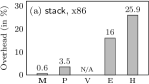
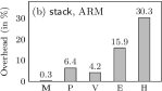
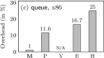
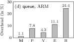
Fig. 1: Overheads for the different fencing strategies

We ran all versions $100$ times, on an x86-64 Intel Core i5-3570 with 4 cores (3.40 GHz) and 4 GB of RAM, and on an ARMv7 (32-bit) Samsung Exynos 4412 with 4 cores (1.6 GHz) and 2 GB of RAM.

For each program version, Fig. 1 shows the mean overhead w.r.t. the unfenced program. We give the overhead (in %) in user time (as given by Linux time), i.e. the time spent by the program in user mode on the CPU. Amongst the approaches that guarantee SC (i.e. all but v), the best results were achieved with our tool musketeer.

We checked the statistical significance of the execution time improvement of our method over the existing methods by computing and comparing the confidence intervals for a sample size of $N=100$ and a confidence level $1-\alpha=95\%$ in Fig. 19. If the confidence intervals for two methods are non-overlapping, we can conclude that the difference between the means is statistically significant.

	stack on x86	stack on ARM	queue on x86	queue on ARM
(o)	[9.757; 9.798]	[11.291; 11.369]	[11.947; 11.978]	[20.441; 20.634]
(m)	[9.818; 9.850]	[11.316; 11.408]	[12.067; 12.099]	[20.687; 20.857]
(p)	[10.077; 10.155]	[11.995; 12.109]	[13.339; 13.373]	[22.035; 22.240]
(v)	N/A	[11.779; 11.834]	N/A	[21.334; 21.526]
(e)	[11.316; 11.360]	[13.071; 13.200]	[13.949, 13.981]	[22.722; 22.903]
(h)	[12.286; 12.325]	[14.676; 14.844]	[14.941, 14.963]	[25.468; 25.633]

Fig. 2: Confidence intervals for data structure experiments.

3 Related work

authors	tool	model style	objective
Abdulla et al. [AAC+13]	memorax	operational	reachability
Alglave et al. [AMSS10]	offence	axiomatic	SC
Bouajjani et al. [BDM13]	trencher	operational	SC
Fang et al. [FLM03]	pensieve	axiomatic	SC
Kuperstein et al. [KVY10]	fender	operational	reachability
Kuperstein et al. [KVY11]	blender	operational	reachability
Linden et al. [LW13]	remmex	operational	reachability
Liu et al. [LNP+12]	dfence	operational	specification
Sura et al. [SFW+05]	pensieve	axiomatic	SC

Fig. 3: Fence synthesis tools

The work of Shasha and Snir [SS88] is a foundation for the field of fence synthesis. Most of the work cited below inherits their notions of delay and critical cycle. A delay is a pair of instructions in a thread that can be reordered by the underlying architecture. A critical cycle essentially represents a minimal violation of SC. Fig. 3 classifies the methods mentioned in this section w.r.t. their style of model (operational or axiomatic). We report our experimental comparison of these tools in Sec. 7. Below, we detail fence synthesis methods per style. We write TSO for Total Store Order, implemented in Sparc TSO [spa94] and Intel x86 [OSS09]. We write PSO for Partial Store Order and RMO for Relaxed Memory Order, two other Sparc architectures. We write Power for IBM Power [ppc09].

Operational models

Linden and Wolper [LW13] explore all executions (using what they call automata acceleration) to simulate the reorderings occuring under TSO and PSO. Abdulla et al. [AAC⁺13] couple predicate abstraction for TSO with a counterexample-guided strategy. They check if an error state is reachable; if so, they calculate what they call the maximal permissive sets of fences that forbid this error state. Their method guarantees that the fences they find are necessary, i.e., removing a fence from the set would make the error state reachable again.

Kuperstein et al. [KVY10] explore all executions for TSO, PSO and a subset of RMO, and along the way build constraints encoding reorderings leading to error states. The fences can be derived from the set of constraints at the error states. The same authors [KVY11] improve this exploration under TSO and PSO using an abstract interpretation they call partial coherence abstraction, relaxing the order in the write buffers after a certain bound, thus reducing the state space to explore. Liu et al. [LNP⁺12] offer a dynamic synthesis approach for TSO and PSO, enumerating the possible sets of fences to prevent an execution picked dynamically from reaching an error state.

Bouajjani et al. [BDM13] build on an operational model of TSO. They look for minimum violations (viz. critical cycles) by enumerating attackers (viz. delays). Like us, they use linear programming. However, they first enumerate all the solutions, then encode them as an ILP, and finally ask the solver to pick the least expensive one. Our method directly encodes the whole decision problem as an ILP. The solver thus both constructs the solution (avoiding the exponential-size ILP problem) and ensures its optimality.

All the approaches above focus on TSO and its siblings PSO and RMO, whereas we also handle the significantly weaker Power, including quite subtle barriers (e.g. lwsync) compared to the simpler mfence of x86.

Axiomatic models

Krishnamurthy et al. [KY96] apply Shasha and Snir’s method to single program multiple data systems. Their abstraction is similar to ours, except that they do not handle pointers.

Lee and Padua [LP01] propose an algorithm based on Shasha and Snir’s work. They use dominators in graphs to determine which fences are redundant. This approach was later implemented by Fang et al. [FLM03] in pensieve, a compiler for Java. Sura et al. later implemented a more precise approach in pensieve [SFW⁺05] (see (p) in Sec. 2). They pair the cycle detection with an analysis to detect synchronisation that could prevent cycles.

Alglave and Maranget [AMSS10] revisit Shasha and Snir for contemporary memory models and insert fences following a refinement of [LP01]. Their offence tool handles snippets of assembly code only, where the memory locations need to be explicitly given.

Others

We cite the work of Vafeiadis and Zappa Nardelli [VZN11], who present an optimisation of the certified CompCert-TSO compiler to remove redundant fences on TSO. Marino et al. [MSM⁺11] experiment with an SC-preserving compiler, showing overheads of no more than $34\,\%$. Nevertheless, they emphasise that “the overheads, however small, might be unacceptable for certain applications”.

4 Axiomatic memory model

mp $T_{0}$ $T_{1}$  $(a)$ $\texttt{x}\leftarrow\texttt{1}$  $(c)$ $\texttt{r1}\leftarrow\texttt{y}$   $(b)$ $\texttt{y}\leftarrow\texttt{1}$  $(d)$ $\texttt{r2}\leftarrow\texttt{x}$    Final state? r1=1 $\wedge$ r2=0

Fig. 4: Message Passing (mp)

Weak memory can occur as follows: a thread sends a write to a store buffer, then a cache, and finally to memory. While the write transits through buffers and caches, a read can occur before the value is available to all threads in memory.

To describe such situations, we use the framework of [AMSS10], embracing in particular SC, Sun TSO (i.e. the x86 model [OSS09]), and a fragment of Power. The core of this framework consists of relations over memory events.

We illustrate this framework using a litmus test (Fig. 4). The top shows a multi-threaded program. The shared variables x and y are assumed to be initialised to zero. A store instruction (e.g. $\texttt{x}\leftarrow\texttt{1}$ on $T_{0}$) gives rise to a write event ($(a)$Wx$1$), and a load instruction (e.g. $\texttt{r1}\leftarrow\texttt{y}$ on $T_{1}$) to a read event ($(c)$Ry1). The bottom of Fig. 4 shows one particular execution of the program (also called event graph), corresponding to the final state r1=1 and r2=0.

In the framework of [AMSS10], an execution that is not possible on SC has a cyclic event graph (as the one shown in Fig. 4). A weaker architecture may relax some of the relations contributing to a cycle. If the removal of the relaxed edges from the event graph makes it acyclic, the architecture allows the execution. For example, Power relaxes the program order po (amongst other things), thereby making the graph in Fig. 4 acyclic. Hence, the given execution is allowed on Power.

Formalisation

An event is a memory read or a write to memory, composed of a unique identifier, a direction (R for read or W for write), a memory address, and a value. We represent each instruction by the events it issues. In Fig. 4, we associate the store instruction $\texttt{$x$}\leftarrow\texttt{1}$ in thread $T_{0}$ with the event $(a)$W$x$$1$.

A set of events $\mathbb{E}$ and their program order po form an event structure ${E}\triangleq{(\mathbb{E},\textsf{po})}$. The program order po is a per-thread total order over $\mathbb{E}$. We write dp (with $\textsf{dp}\subseteq\textsf{po}$) for the relation that models dependencies between instructions. For instance, there is a data dependency between a load and a store when the value written by the store was computed from the value obtained by the load.

We represent the communication between threads via an execution witness ${X}\triangleq{(\textsf{co},\textsf{rf})}$, which consists of two relations over the events. First, the coherence co is a per-address total order on write events which models the memory coherence widely assumed by modern architectures. It links a write $w$ to any write $w^{\prime}$ to the same address that hits the memory after $w$. Second, the read-from relation rf links a write $w$ to a read $r$ such that $r$ reads the value written by $w$. Finally, we derive the from-read relation fr from co and rf. A read $r$ is in fr with a write $w$ if the write $w^{\prime}$ from which $r$ reads hits the memory before $w$. Formally, we have: ${(r,w)\in\textsf{fr}}\triangleq{\exists w^{\prime}.(w^{\prime},r)\in\textsf{rf}\wedge(w^{\prime},w)\in\textsf{co}}$.

In Fig. 4, the specified outcome corresponds to the execution below if each location initially holds $0$. If r1=1 in the end, the read $(c)$ on $T_{1}$ took its value from the write $(b)$ on $T_{0}$, hence $(b,c)\in\textsf{rf}$. If r2=0 in the end, the read $(d)$ took its value from the initial state, thus before the write $(a)$ on $T_{0}$, hence $(d,a)\in\textsf{fr}$. In the following, we write rfe (resp. $\textsf{coe},\textsf{fre}$) for the external read-from (resp. coherence, from-read), i.e. when the source and target belong to different threads.

	SC	x86	Power
poWR	yes	mfence	sync
poWW	yes	yes	sync, lwsync
poRW	yes	yes	sync, lwsync, dp
poRR	yes	yes	sync, lwsync, dp, branch;isync

Fig. 5: ppo and fences per architecture

Relaxed or safe

We model the scenario of reads occurring in advance, as described at the beginning of this section, by some subrelation of the read-from rf being relaxed, i.e. not included in global happens before. When a thread can read from its own store buffer [AG95] (the typical TSO/x86 scenario), we relax the internal read-from, that is, rf where source and target belong to the same thread. When two threads $T_{0}$ and $T_{1}$ can communicate privately via a cache (a case of write atomicity relaxation [AG95]), we relax the external read-from rfe, and call the corresponding write non-atomic. This is the main particularity of Power and ARM, and cannot happen on TSO/x86. Some program-order pairs may be relaxed (e.g. write-read pairs on x86, and all but dp ones on Power), i.e. only a subset of po is guaranteed to occur in order. This subset constitutes the preserved program order, ppo. When a relation must not be relaxed on a given architecture, we call it safe.

Fig. 5 summarises ppo per architecture. The columns are architectures, e.g. x86, and the lines are relations, e.g. poWR. We write e.g. poWR for the program order between a write and a read. We write “yes” when the relation is in the ppo of the architecture: e.g. poWR is in the ppo of SC. When we write something else, typically the name of a fence, e.g. mfence, the relation is not in the ppo of the architecture (e.g. poWR is not in the ppo of x86), and the fence can restore the ordering: e.g. mfence maintains write-read pairs in program order.

Following [AMSS10], the relation fence (with $\textsf{fence}\subseteq{\textsf{po}}$) induced by a fence is non-cumulative when it only orders certain pairs of events surrounding the fence. The relation fence is cumulative when it additionally makes writes atomic, e.g. by flushing caches. In our model, this amounts to making sequences of external read-from and fences ($\textsf{rfe};\textsf{fence}$ or $\textsf{fence};\textsf{rfe}$) safe, even though rfe alone would not be safe. In Fig. 4, placing a cumulative fence between the two writes on $T_{0}$ will not only prevent their reordering, but also enforce an ordering between the write $(a)$ on $T_{0}$ and the read $(c)$ on $T_{1}$, which reads from $T_{0}$.

Architectures

An architecture $A$ determines the set $\operatorname{safe}_{A}$ of relations safe on $A$. Following [AMSS10], we always consider the coherence co, the from-read relation fr and the fences to be safe. SC relaxes nothing, i.e. rf and po are safe. TSO authorises the reordering of write-read pairs and store buffering but nothing else.

Critical cycles

Following [SS88, AM11], for an architecture $A$, a delay is a po or rf edge that is not safe (i.e. is relaxed) on $A$. An execution $(E,X)$ is valid on $A$ yet not on SC iff it contains critical cycles [AM11]. Formally, a critical cycle w.r.t. $A$ is a cycle in ${\textsf{po}{}}\cup{\textsf{com}{}}$, where ${\textsf{com}}\leavevmode\nobreak\ \triangleq\leavevmode\nobreak\ {\textsf{co}\cup\textsf{rf}\cup\textsf{fr}}$ is the communication relation, which has the following characteristics (the last two ensure the minimality of the critical cycles): (1) the cycle contains at least one delay for $A$; (2) per thread, (i) there are at most two accesses $a$ and $b$, and (ii) they access distinct memory locations; and (3) for a memory location $\ell$, there are at most three accesses to $\ell$ along the cycle, which belong to distinct threads.

Fig. 4 shows a critical cycle w.r.t. Power. The po edge on $T_{0}$, the po edge on $T_{1}$, and the rf edge between $T_{0}$ and $T_{1}$, are all unsafe on Power. On the other hand, the cycle in Fig. 4 does not contain a delay w.r.t. TSO, and is thus not a critical cycle on TSO.

To forbid executions containing critical cycles, one can insert fences into the program to prevent delays. To prevent a po delay, a fence can be inserted between the two accesses forming the delay, following Fig. 5. To prevent an rf delay, a cumulative fence must be used (see Sec. 6 for details). For the example in Fig. 4, for Power, we need to place a cumulative fence between the two writes on $T_{0}$, preventing both the po and the adjacent rf edge from being relaxed, and use a dependency or fence to prevent the po edge on $T_{1}$ from being relaxed.

5 Static detection of critical cycles

We want to synthesise fences to prevent weak behaviours and thus restore SC. We explained in Sec. 4 that we should place fences along the critical cycles of the program executions. To find the critical cycles, we look for cycles in an over-approximation of all the executions of the program. We hence avoid enumeration of all traces, which would hinder scalability, and get all the critical cycles of all program executions at once. Thus we can find all fences preventing the critical cycles corresponding to two executions in one step, instead of examining the two executions separately.

⬇ void thread_1(int input) { int r1; x = input; if(rand()%2) y = 1; else r1 = z; x = 1; } void thread_2() { int r2, r3, r4; r2 = y; r3 = z; r4 = x; } . . .

⬇ thread_1 int r1; x = input; _Bool tmp; tmp = rand(); [!tmp%2] goto 1; y = 1; goto 2; 1: r1 = z; 2: x = 1; end_function thread_2 int r2, r3, r4; r2 = y; r3 = z; r4 = x; end_function . . . . .

Fig. 6: A C program (left) and its goto-program (right)

To analyse a C program, e.g. on the left-hand side of Fig. 6, we convert it to a goto-program (right-hand side of Fig. 6), the internal representation of the CProver framework; we refer to http://www.cprover.org/goto-cc for details. The pointer analysis we use is a standard concurrent points-to analysis that we have shown to be sound for our weak memory models in earlier work [AKL⁺11]. We explain in details how we handle pointers at the end of this section. The C program in Fig. 6 features two threads which can interfere. The first thread writes the argument “input” to $x$, then randomly writes $1$ to $y$ or reads $z$, and then writes $1$ to $x$. The second thread successively reads $y$, $z$ and $x$. In the corresponding goto-program, the if-else structure has been transformed into a guard with the condition of the if followed by a goto construct. From the goto-program, we then compute an abstract event graph (aeg), shown in Fig. 7(a). The events $a,b_{1},b_{2}$ and $c$ (resp. $d,e$ and $f$) correspond to thread₁ (resp. thread₂) in Fig. 6. We only consider accesses to shared variables, and ignore the local variables. We finally explore the aeg to find the potential critical cycles.

An aeg represents all the executions of a program (in the sense of Sec. 4). Fig. 7(b) and (c) give two executions associated with the aeg shown in Fig. 7(a). For readability, the transitive po edges have been omitted (e.g. between the two events $d^{\prime}$ and $f^{\prime}$). The concrete events that occur in an execution are shown in bold. In an aeg, the events do not have concrete values, whereas in an execution they do. Also, an aeg merely indicates that two accesses to the same variable could form a data race (see the competing pairs ($\operatorname{\textsf{cmp}}$) relation in Fig. 7(a), which is a symmetric relation), whereas an execution has oriented relations (e.g. indicating the write that a read takes its value from, see e.g. the rf arrow in Fig. 7(b) and (c)). The execution in Fig. 7(b) has a critical cycle (with respect to e.g. Power) between the events $a^{\prime}$, $b_{2}^{\prime}$, $d^{\prime}$, and $f^{\prime}$. The execution in Fig. 7(c) does not have a critical cycle.

We build an aeg essentially as in [AKNT13]. However, our goal and theirs are not the same: they instrument an input program to reuse SC verification tools to perform weak memory verification, whereas we are interested in automatic fence placement. Moreover, the work of [AKNT13] did not present a semantics of goto-programs in terms of aegs, which we do in this section.

(a) aeg of Fig. 6	(b) ex. with critical cycle	(c) ex. without critical cycle

Fig. 7: The aeg of Fig. 6 and two executions corresponding to it

(1) assignment: $lhs$=$rhs$; $i$
$\tau[lhs=rhs;i](aeg)=\tau[i]((aeg.\mathbb{E}_{s}\cup\text{evts}(lhs)\cup\text{evts}(rhs),aeg.\text{{po}${}_{s}${}}\cup\text{end}(aeg.\text{{po}${}_{s}${}})\times(\text{evts}(rhs)\cup\text{evts}(lhs)\backslash\text{trg}(lhs))\cup(\text{evts}(rhs)\cup\text{evts}(lhs)\backslash\text{trg}(lhs))\times\text{trg}(lhs),aeg.\operatorname{\textsf{cmp}}))$
(2) function call: $fun$(); $i$
$\tau[fun();i]=\tau[i]\circ\tau[\text{body}(fun)]$
(3) guard: [$expr$] $i_{1}$; $i_{2}$
$\tau[[guard]i_{1};i_{2}](aeg)=$ let guarded$=\tau[i_{1}](aeg)$ in $\tau[i_{2}]((aeg.\mathbb{E}_{s}\cup\text{guarded}.\mathbb{E}_{s},aeg.\text{{po}${}_{s}${}}\cup\text{guarded}.\text{{po}${}_{s}${}},aeg.\operatorname{\textsf{cmp}}))$
(4) forward jump:  goto $l$;
$\tau[goto\,\,l;i]=\tau[\text{follow}(l)]$
(5) backward jump: $l$: $i_{1}$; [$cond$] goto $l$; $i_{2}$
$\tau[l:i_{1};[cond]\text{goto}\,\,l;i_{2}](aeg)=$ let local$=\tau[i_{1}](aeg)$ in $\tau[i_{2}]((aeg.\mathbb{E}_{s}\cup\text{local}.\mathbb{E}_{s},aeg.\text{{po}${}_{s}${}}\cup\text{local}.\text{{po}${}_{s}${}}\cup\text{end}(\text{local}.\text{{po}${}_{s}${}})\times\text{begin}(\text{local}.\text{{po}${}_{s}${}}),aeg.\operatorname{\textsf{cmp}}))$
(6) assume / assert / skip:  assume($\phi$); $i$ / assert($\phi$); $i$ / skip; $i$
$\tau[assume(\phi);i]=\tau[i]$
(7) atomic section: atomic_begin; $i_{1};$ atomic_end; $i_{2}$
$\tau[atomic\_start;i_{1};atomic\_end;i_{2}](aeg)=$ let section=$\tau[i_{1}]((aeg.\mathbb{E}_{s},aeg.\text{{po}${}_{s}${}}\cup\text{end}(aeg.\text{{po}${}_{s}${}})\times\{\textsf{f}\},aeg.\operatorname{\textsf{cmp}}))$ in $\tau[i_{2}]((\text{section}.\mathbb{E}_{s},\text{section}.\text{{po}${}_{s}${}}\cup\text{end}(\text{section}.\text{{po}${}_{s}${}})\times\{\textsf{f}\},\text{section}.\operatorname{\textsf{cmp}}))$
(8) new thread: start_thread $th$; $i$
$\tau[start\_thread\,\,th;i](aeg)=$ let local=$\tau[\text{body}(th)](\bar{\emptyset})$ and main=$\tau[i](aeg)$ and inter=$\tau[i](\bar{\emptyset})$ in $(\text{local}.\mathbb{E}_{s}\cup\text{main}.\mathbb{E}_{s},\text{local}.\text{{po}${}_{s}${}}\cup\text{main}.\text{{po}${}_{s}${}},\text{local}.\mathbb{E}_{s}\otimes\text{inter}.\mathbb{E}_{s})$
(9) end of thread: end_thread;
$\tau[end\_thread](aeg)=aeg$	$\emptyset$

Fig. 8: Operations to create the aeg of a goto-program

Constructing aegs

For each goto-program(e.g. bottom of Fig. 6),we build an aeg $\triangleq({\mathbb{E}}_{s},\text{{po}${}_{s}$},\operatorname{\textsf{cmp}})$ as follows (see Fig. 7(a)), with the abstract events ${\mathbb{E}}_{s}$, the static program order po_s and the competing pairs $\operatorname{\textsf{cmp}}$. Given an aeg $G$, we write respectively $G.{\mathbb{E}}_{s}$, $G.$po_s and $G.\operatorname{\textsf{cmp}}{}$ for the abstract events, the static program order and the competing pairs of $G$.

An abstract event ​​​

represents all events with same program point, memory location and direction (write or read). In Fig. 7(a), ($a$)Wx abstracts the events ($a^{\prime}$)Wx1 and ($a^{\prime\prime}$)Wx2 in the executions of Fig. 7(b) and (c).

The static program order po_s ​​​

abstracts all the (dynamic) po edges that connect two events in program order and that cannot be decomposed as a succession of po edges in this execution. We write po${}_{s}^{+}$ (resp. po${}_{s}^{*}$) for the transitive (resp. reflexive transitive) closure of this relation.

The competing pairs ​​​

$\operatorname{\textsf{cmp}}$ over-approximate the external communications ${\textsf{coe}}\cup{\textsf{rfe}}\cup{\textsf{fre}}$. In Fig. 7(a), the $\operatorname{\textsf{cmp}}$ edges $(a,f)$, $(b_{1},d)$, and $(c,f)$ abstract in particular the fre edges $(f^{\prime},c^{\prime})$ and $(f^{\prime},a^{\prime})$, and the rfe edge $(b_{1}^{\prime},d^{\prime})$ in Fig. 7(b). We do not need to represent internal communications as they are already covered by po${}_{s}^{+}$. The cmp construction is similar to the first steps of static data race detections (see [KSKZ09, Sec. 5]), where shared variables involved in write-read or write-write communications are collected.

To build the aeg​​​​

, we define a semantics of goto-programs in terms of abstract events, static program order and competing pairs. We detail below this semantics for each goto-statement. Each of these cases is accompanied in Fig. 8 by a graphical representation summarising the aeg construction on the right-hand side, and a formal definition of the semantics on the left-hand side. In Fig. 8, we write $\tau[i]$ to represent the semantics of a goto-instruction $i$. Other notations, e.g. follow(f) or body(f), are explained below. We do not compute the values of our variables, and thus do not interpret the expressions. In Fig. 7(a), ($a$)Wx represents the assignment “x = input” in thread 1 in Fig. 6 (since “input” is a local variable). This abstracts the values that “input” could hold, e.g. 1 (see ($a^{\prime}$)Wx1 in Fig. 7(b)) or 2 (see ($a^{\prime\prime}$)Wx2 in Fig. 7(c)). Prior to building the aeg, we copy expressions of conditions or function arguments into local variables. Thus all the work over shared variables is handled in the assignment case.

We now present the construction of the aeg starting with the intra-thread instructions (e.g. assignments, function calls), creating po_s edges, then the thread constructor, creating $\operatorname{\textsf{cmp}}{}$ edges.

Assignments lhs=rhs We decompose this statement into sets of abstract events: the reads from shared variables in rhs and lhs, denoted by evts(rhs) and evts(lhs), and the writes to the potential target objects trg(lhs) (determined from lhs as explained below). We do not assume any order in the evaluation of the variables in an expression. Hence, we connect to the incoming po_s all the reads of rhs and all the reads of lhs except trg(lhs). We then connect each of them to the potential target writes to trg(lhs). This is the set of objects (in the C sense [c1111]) that could be written to, according to our pointer analysis. They are either fields of structures, structures, arrays (independent of their offsets) or variables. If we have e.g. *(&t+y+r)=z+3 (where t, y and z are shared), t is our target variable, and we obtain $(R\texttt{y},W\texttt{t})\in$ po_s and $(R\texttt{z},W\texttt{t})\in$ po_s. We also maintain a map from local to shared variables, to record the data and address dependencies between abstract events.

Procedure calls fun() We build the po_s corresponding to the function’s body (written body(fun)) once and for all. We then replace the call to a function fun() by its body. This ensures a better precision, in the sense that a function can be fenced in a given context and unfenced in another.

Guarded statement We do not keep track of the values of the variables at each program point. Thus we cannot evaluate the guard of a statement. Hence, we abstract the guard and make this statement non-deterministically reachable, by adding a second po_s edge, bypassing the statement.

Forward jump to a label $L$ We connect the previous abstract events to the next abstract events that we generate from the program point $L$. In Fig. 8, we write follow($L$) for the sequence of statements following the label $L$.

Backward jump (unbounded loops), i.e., a jump to a label already visited. We connect the last abstract event of the copy to the first abstract event of the original body with a po_s edge. In Fig. 8, begin($S$) and end($S$) are respectively the sets of the first and last abstract events of the po_s sub-graph $S$.

Assumption Similarly to the guarded statement, as we cannot evaluate the condition, we abstract the assumptions by bypassing them.

Atomic sections ​ are special goto-instructions, for modelling idealised atomic sections without having to rely on the correctness of their implementation. These are used in many theoretical concurrency and verification works. For example, we use them (see Sec. 7) for copying data to atomic structures, as in e.g. our implementation of the Chase-Lev queue [CL05]. Reorderings cannot happen across an atomic section, thus we place two full fences f right after the beginning of the section and just before the end of section.

Construction of cmp During the construction of po_s, we also compute the competing pairs that abstract external communications between threads. For each write $w$ to a memory location $x$, we augment the $\operatorname{\textsf{cmp}}$ relation with pairs made of this write and any write to $x$ from an interfering thread: this abstracts the coherence coe. Similarly, we augment $\operatorname{\textsf{cmp}}$ with pairs made of $w$ and any read of $x$ from an interfering thread. Symmetrically, for each read $r$ of $y$, we add pairs made of $r$ and any write to $y$ from an interfering thread to $\operatorname{\textsf{cmp}}$. This abstracts the from-read fre and read-from rfe relations. In Fig. 8, we use $\otimes$ to construct the $\operatorname{\textsf{cmp}}$ edges when encountering a new interfering thread spawned, that is, when the goto-instruction start_thread is met. We define $\otimes$ as $A\otimes B=\{(x,y)|(x,y)\in A\times B\text{ s.t. }write(x)\lor write(y)\}$. $\bar{\emptyset}$ stands for the triplet $(\emptyset,\emptyset,\emptyset)$.

Interplay with pointer analyses

We explain how to deal with the varying imprecision of pointer analyses in a sound way. We want to find all critical cycles in the static aeg. Yet, some cycles might reveal themselves only dynamically, e.g., across several iterations of a same loop. Fig. 9a gives an aeg for a two-thread program, where the first thread loops and writes to a shared array t and the second thread reads from this array.

This program could exhibit a message passing pattern (see Fig. 4), where writes in the loop could be reordered. If we build our aeg following the cfg, we obtain one abstract event for all writes of the loop. How we address this depends on the precision of our pointer analysis.

If we have a precise pointer analysis, we insert as many abstract events as required for the objects pointed to, as in Fig. 9b. Otherwise, we underspecify the abstract event: in Fig. 9c, we abstract Wt[i] by Wt[*]. We then replicate the body of the loop, hence the two Wt[*] in po_s. They abstract any two writes to distinct places in t that could occur across the iterations, as required by (2.i) and (2.ii) above. Our tool musketeer implements this method.

If the analysis cannot determine the location of an access, we insert an abstract event accessing any shared variable, as in Fig. 9d. This event can communicate with any variable accessed in other threads.

(a) aeg following directly the cfg		(b) aeg with a precise p.a.
(c) aeg with an index-insensitive p.a.		(d) aeg with an imprecise p.a.

Fig. 9: Construction of aeg for dynamic cycles w.r.t. pointer analysis (p.a.) precision

Cycle detection

Once we have the aeg, we enumerate (using Tarjan’s algorithm [Tar73]) its potential critical cycles by searching for cycles that contain at least one edge that is a delay, as defined in Sec. 4.

6 Synthesis

$\begin{array}[]{l l l}\text{{min} }&\lx@intercol\text{\tt dp}_{(e,g)}+\text{\tt dp}_{(f,h)}+\text{\tt dp}_{(f,g)}+3\cdot(\text{\tt f}_{(e,f)}+\text{\tt f}_{(f,g)}+\text{\tt f}_{(g,h)})+2\cdot(\text{\tt lwf}_{(e,f)}+\text{\tt lwf}_{(f,g)}+\text{\tt lwf}_{(g,h)})\hfil\lx@intercol\\ \text{{s.t.}}&\text{cycle 1, delay $(e,g)$:}&\text{\tt dp}_{(e,g)}+\text{\tt f}_{(e,f)}+\text{\tt f}_{(f,g)}+\text{\tt lwf}_{(e,f)}+\text{\tt lwf}_{(f,g)}\geq 1\\ &\text{cycle 2, delay $(f,g)$:}&\text{\tt dp}_{(f,g)}+\text{\tt f}_{(f,g)}+\text{\tt lwf}_{(f,g)}\geq 1\\ &\text{cycle 3, delay $(f,h)$:}&\text{\tt dp}_{(f,h)}+\text{\tt f}_{(f,g)}+\text{\tt f}_{(g,h)}+\text{\tt lwf}_{(f,g)}+\text{\tt lwf}_{(g,h)}\geq 1\\ &\text{cycle 4, delay $(g,h)$:}&\text{\tt f}_{(g,h)}\geq 1\end{array}$

Fig. 10: Example of resolution with $\operatorname{\textsf{between}}$

In Fig. 10, we have an aeg with five threads: $\{a,b\},\{c,d\}$, $\{e,f,g,h\}$, $\{i,j\}$ and $\{k,l\}$. Each node is an abstract event computed as in the previous section. The dashed edges represent the po_s between abstract events in the same thread. The full lines represent the edges involved in a cycle. Thus the aeg of Fig. 10 has four potential critical cycles. We derive the set of constraints in a process we define later in this section. We now have a set of cycles to forbid by placing fences. Moreover, we want to optimise the placement of the fences.

Challenges

If there is only one type of fence (as in TSO, which only features mfence), optimising only consists of placing a minimal amount of fences to forbid as many cycles as possible. For example, placing a full fence sync between $f$ and $g$ in Fig. 10 might forbid cycles 1, 2 and 3 under Power, whereas placing it somewhere else might forbid at best two amongst them.

Since we handle several types of fences for a given architecture (e.g. dependencies, lwsync and sync on Power), we can also assign some cost to each of them. For example, following the folklore, a dependency is less costly than an lwsync, which is itself less costly than a sync. Given these costs, one might want to minimise their sum along different executions: to forbid cycles 1, 2 and 3 in Fig. 10, a single lwsync between $f$ and $g$ can be cheaper at runtime than three dependencies respectively between $e$ and $g$, $f$ and $g$, and $f$ and $h$. However, if we had only cycles 1 and 2, the dependencies would be cheaper. We see that we have to optimise both the placement and the type of fences at the same time.

Input: aeg ($\mathbbm{E}_{s}$,po_s,$\operatorname{\textsf{cmp}}$) and potential critical cycles   $C=\{C_{1},...,C_{n}\}$ Problem: minimise $\sum_{(l,\textsf{t})\in\operatorname{\textsf{potential-places}}(C)}\textsf{t}_{l}\times\operatorname{\textsf{cost}}(\textsf{t})$ Constraints: for all $d\in\text{delays}(C)$ (* for TSO, PSO, RMO, Power *) if $d\in\textsf{poWR}$ then $\sum_{e\in\operatorname{\textsf{between}}(d)}{\textsf{f}}_{e}\geq 1$ if $d\in\textsf{poWW}$ then $\sum_{e\in\operatorname{\textsf{between}}(d)}{\textsf{f}}_{e}+\textsf{lwf}_{e}\geq 1$ if $d\in\textsf{poRW}$ then $\textsf{dp}_{d}+\sum_{e\in\operatorname{\textsf{between}}(d)}{\textsf{f}}_{e}+\textsf{lwf}_{e}\geq 1$ if $d\in\textsf{poRR}$ then $\textsf{dp}_{d}+\sum_{e\in\operatorname{\textsf{between}}(d)}{\textsf{f}}_{e}+\textsf{lwf}_{e}\quad+\sum_{e\in\operatorname{\textsf{ctrl}}(d)}\textsf{cf}_{e}\geq 1$ (* for Power *) if $d\in\operatorname{\textsf{cmp}}$ then $\sum_{e\in\operatorname{\textsf{cumul}}(d)}{\textsf{f}}_{e}+\sum_{e\in\operatorname{\textsf{cumul}}(d)\cap\neg\textsf{poWR}\cap\neg\textsf{poRW}}\textsf{lwf}_{e}\geq 1$ Output: the set $\operatorname{\textsf{actual-places}}(C)$ of pairs $(l,\textsf{t})$ s.t. $\textsf{t}_{l}$ is set to 1 in the ILP solution

Fig. 11: ILP for inferring fence placements

We model our problem as an integer linear program (ILP) (see Fig. 11), which we explain in this section. Solving our ILP gives us a set of fences to insert to forbid the cycles. This set of fences is optimal in that it minimises the cost function. More precisely, the constraints are the cycles to forbid, each variable represents a fence to insert, and the cost function sums the cost of all fences.

6.1 Cost function of the ILP

We handle several types of fences: full (f), lightweight (lwf), control fences (cf), and dependencies (dp). On Power, the full fence is sync, the lightweight one lwsync. We write $\mathbb{T}$ for the set $\{\textsf{dp},\textsf{f},\textsf{cf},\textsf{lwf}\}$. We assume that each type of fence has an a priori cost (e.g. a dependency is cheaper than a full fence), regardless of its location in the code. We write $\operatorname{\textsf{cost}}(\textsf{t})$ for $\textsf{t}\in\mathbb{T}$ for this cost.

We take as input the aeg of our program and the potential critical cycles to fence. We define two sets of pairs $(l,\textsf{t})$ where $l$ is a po_s edge of the aeg and t a type of fence. We introduce an ILP variable $\mathsf{t}_{l}$ (in $\{0,1\}$) for each pair $(l,\textsf{t})$.

The set $\operatorname{\textsf{potential-places}}$ is the set of such pairs that can be inserted into the program to forbid the cycles. The set $\operatorname{\textsf{actual-places}}$ is the set of such pairs that have been set to $1$ by our ILP. We output this set, as it represents the locations in the code in need of a fence and the type of fence to insert for each of them. We also output the total cost of all these insertions, i.e. $\sum_{(l,\textsf{t})\in\operatorname{\textsf{potential-places}}(C)}\textsf{t}_{l}\times\operatorname{\textsf{cost}}(\textsf{t})$. The solver should minimise this sum whilst satisfying the constraints.

6.2 Constraints in the ILP

We want to forbid all the cycles in the set that we are given after filtering, as explained in the preamble of this section. This requires placing an appropriate fence on each delay for each cycle in this set. Different delay pairs might need different fences, depending e.g. on the directions (write or read) of their extremities. Essentially, we follow the table in Fig. 5. For example, a write-read pair needs a full fence (e.g. mfence on x86, or sync on Power). A read-read pair can use anything amongst dependencies and fences. Our constraints ensure that we use the right type of fence for each delay pair.

Inequalities as constraints

We first assume that all the program order delays are in po_s and we ignore Power and ARM special features (dependencies, control fences and communication delays). This case deals with relatively strong models, ranging from TSO to RMO. We relax these assumptions below.

In this setting, $\operatorname{\textsf{potential-places}}(C)$ is the set of all the po_s delays of the cycles in $C$. We ensure that every delay pair for every execution is fenced, by placing a fence on the static po_s edge for this pair, and this for each cycle given as input. Thus, we need at least one constraint per static delay pair $d$ in each cycle.

If $d$ is of the form poWR, as $(g,h)$ in Fig. 10 (cycle 4), only a full fence can fix it (cf. Fig. 5), thus we impose $\textsf{f}_{d}\geq 1$. If $d$ is of the form poRR, as $(f,h)$ in Fig. 10 (cycle 3), we can choose any type of fence, i.e. $\textsf{dp}_{d}+\textsf{cf}_{d}+\textsf{lwf}_{d}+\textsf{f}_{d}\geq 1$.

Our constraints cannot be equalities because it is not certain that the resulting system would be satisfiable. To see this, suppose our constraints were equalities, and consider Fig. 10 limited to cycles 2, 3 and 4. Using only full fences, lightweight fences, and dependencies (i.e. ignoring control fences for now), we would generate the constraints (i) $\textsf{lwf}_{(f,g)}+\textsf{f}_{(f,g)}=1$ for the delay $(f,g)$ in cycle 2, (ii) $\textsf{dp}_{(f,h)}+\textsf{lwf}_{(f,h)}+\textsf{f}_{(f,h)}+\textsf{lwf}_{(g,h)}+\textsf{f}_{(g,h)}=1$ for the delay $(f,h)$ in cycle 3, and (iii) $\textsf{f}_{(g,h)}=1$ for the delay $(g,h)$ in cycle 4.

Preventing the delay $(g,h)$ in cycle 4 requires a full fence, thus $\textsf{f}_{(g,h)}=1$. By the constraint (ii), and since $\textsf{f}_{(g,h)}=1$, we derive $\textsf{f}_{(f,g)}=0$ and $\textsf{lwf}_{(f,g)}=0$. But these two equalities are not possible given the constraint (i). By using inequalities, we allow several fences to live on the same edge. In fact, the constraints only ensure the soundness; the optimality is fully determined by the cost function to minimise.

Delays ​​​

are in fact in po${}_{s}^{+}$, not always in po_s: in Fig. 10, the delay $(e,g)$ in cycle 1 does not belong to po_s but to po${}_{s}^{+}$. Thus given a po${}_{s}^{+}$ delay $(x,y)$, we consider all the po_s pairs which appear between $x$ and $y$, i.e.: $\operatorname{\textsf{between}}(x,y)\triangleq\{(e_{1},e_{2})\in\text{{po}${}_{s}${}}\mid(x,e_{1})\in\text{{po}${}_{s}^{*}$}\land(e_{2},y)\in\text{{po}${}_{s}^{*}$}\}.$ For example in Fig. 10, we have $\operatorname{\textsf{between}}(e,g)=\{(e,f),\,(f,g)\}$. Thus, ignoring the use of dependencies and control fences for now, for the delay $(e,g)$ in Fig. 10, we will not impose $\textsf{f}_{(e,g)}+\textsf{lwf}_{(e,g)}\geq 1$ but rather $\textsf{f}_{(e,f)}+\textsf{lwf}_{(e,f)}+\textsf{f}_{(f,g)}+\textsf{lwf}_{(f,g)}\geq 1$. Indeed, a full fence or a lightweight fence in $(e,f)$ or $(f,g)$ will prevent the delay in $(e,g)$.

Dependencies ​​​​

need more care, as they cannot necessarily be placed anywhere between $e$ and $g$ (in the formal sense of $\operatorname{\textsf{between}}(e,g)$): $\textsf{dp}_{(e,f)}$ or $\textsf{dp}_{(f,g)}$ would not fix the delay $(e,g)$, but simply maintain the pairs $(e,f)$ or $(f,g)$, leaving the pair $(e,g)$ free to be reordered. Thus if we choose to synchronise $(e,g)$ using dependencies, we actually need a dependency from $e$ to $g$: $\textsf{dp}_{(e,g)}$. Dependencies only apply to pairs that start with a read; thus for each such pair (see the poRW and poRR cases in Fig. 11), we add a variable for the dependency: $(e,g)$ will be fixed with the constraint $\textsf{dp}_{(e,g)}+\textsf{f}_{(e,f)}+\textsf{lwf}_{(e,f)}+\textsf{f}_{(f,g)}+\textsf{lwf}_{(f,g)}\geq 1$.

Control fences ​​

placed after a conditional branch (e.g. bne on Power) prevent speculative reads after this branch (see Fig. 5). Thus, when building the aeg, we built a set poC for each branch, which gathers all the pairs of abstract events such that the first one is the last event before a branch, and the second is the first event after that branch. We can place a control fence before the second component of each such pair, if the second component is a read. Thus, we add $\textsf{cf}_{e}$ as a possible variable to the constraint for read-read pairs (see poRR case in Fig. 11, where $\operatorname{\textsf{ctrl}}(d)=\operatorname{\textsf{between}}(d)\cap\textsf{poC}{}$).

Cumulativity

For architectures like Power, where stores are non-atomic, we need to look for program order pairs that are connected to an external read-from (e.g. $(c,d)$ in Fig. 4 has an rf connected to it via event $c$). In such cases, we need to use a cumulative fence, e.g. lwsync or sync, and not, for example, a dependency.

The locations to consider in such cases are: before (in po_s) the write $w$ of the rfe, or after (in po_s) the read $r$ of the rfe, i.e. $\operatorname{\textsf{cumul}}(w,r)=\{(e_{1},e_{2})\mid(e_{1},e_{2})\in\text{{po}${}_{s}$}\land((e_{2},w)\in\text{{po}${}_{s}^{*}$}\lor(r,e_{1})\in\text{{po}${}_{s}^{*}$})\}$. In Fig. 10 (cycle 2), $(g,i)$ over-approximates an rfe edge, and the edges where we can insert fences are in $\operatorname{\textsf{cumul}}(g,i)=\{(f,g),\,(i,j)\}$.

We need a cumulative fence as soon as there is a potential rfe, even if the adjacent po_s pairs do not form a delay. For example in Fig. 4, suppose there is a dependency between the reads on $T_{1}$, and a fence maintaining write-write pairs on $T_{0}$. In that case we need to place a cumulative fence to fix the rfe, even if the two po_s pairs are themselves fixed. Thus, we quantify over all po_s pairs when we need to place cumulative fences. As only f and lwf are cumulative, we have $\operatorname{\textsf{potential-places}}(C)\triangleq$ $\left\{(l,t)\mid(t\in\{\textsf{dp}\}\right.$ $\land\leavevmode\nobreak\ l\in\text{delays}(C))$ $\lor(t\in\mathbb{T}\backslash\{\textsf{dp}\}$ $\land\leavevmode\nobreak\ l\in\bigcup_{d\in\text{delays}(C)}\operatorname{\textsf{between}}(d))$ $\lor(t\in\{\textsf{f},\textsf{lwf}\}$ $\left.\land\leavevmode\nobreak\ l\in\text{{po}${}_{s}$}(C))\right\}$.

6.3 Comparison with trencher

Fig. 12: Cycles sharing the edge $(a,b)$

We illustrate the difference between trencher [BDM13] and our approach using Fig. 12. There are three cycles that share the edge $(a,b)$. They differ in the path taken between nodes $c$ and $g$. Suppose that the user has inserted a full fence between $a$ and $b$. To forbid the three cycles, we need to fence the thread on the right.

The trencher algorithm first calculates which pairs can be reordered: in our example, these are $(c,g)$ via $d$, $(c,g)$ via $e$ and $(c,g)$ via $f$. It then determines at which locations a fence could be placed. In our example, there are $6$ options: $(c,d)$, $(d,g)$, $(c,e)$, $(e,g)$, $(c,f)$, and $(f,g)$. The encoding thus uses $6$ variables for the fence locations. The algorithm then gathers all the irreducible sets of locations to be fenced to forbid the delay between $c$ and $g$, where “irreducible” means that removing any of the fences would prevent this set from fully fixing the delay. As all the paths that connect $c$ and $g$ have to be covered, trencher needs to collect all the combinations of one fence per path. There are $2$ locations per path, leading to $2^{3}$ sets. Consequently, as stated in [BDM13], trencher needs to construct an exponential number of sets.

Each set is encoded in the ILP with one variable. For this example, trencher thus uses $6+8$ variables. It also generates one constraint per delay (here, $1$) to force the solver to pick a set, and $8$ constraints to enforce that all the location variables are set to $1$ if the set containing these locations is picked.

By contrast, musketeer only needs $6$ variables: the possible locations for fences. We detect three cycles, and generate only three constraints to fix the delay. Thus, on a parametric version of the example, trencher’s ILP grows exponentially whereas musketeer’s is linear-sized.

7 Implementation, Experiments and Impact

	classic										fast
	Dek		Pet		Lam		Szy		Par		Cil		CL		Fif		Lif		Anc		Har
LoC	50		37		72		54		96		97		111		150		152		188		179
dfence	–	–	–	–	–	–	–	–	–	–	7.8	3	6.2	3	$\sim$	0	$\sim$	0	$\sim$	0	$\sim$	0
memorax	0.4	2	1.4	2	79.1	4	–	–	–	–	–	–	–	–	–	–	–	–	–	–	–	–
musketeer	0.0	5	0.0	3	0.0	8	0.0	8	0.0	3	0.0	3	0.0	1	0.1	1	0.0	1	0.1	1	0.6	4
offence	0.0	2	0.0	2	0.0	8	0.0	8	–	–	–	–	–	–	–	–	–	–	–	–	–	–
pensieve	0.0	16	0.0	6	0.0	24	0.0	22	0.0	7	0.0	14	0.0	8	0.1	33	0.0	29	0.0	44	0.1	72
remmex	0.5	2	0.5	2	2.0	4	1.8	5	–	–	–	–	–	–	–	–	–	–	–	–	–	–
trencher	1.6	2	1.3	2	1.7	4	–	–	0.5	1	8.6	3	–	–	–	–	–	–	–	–	–	–

Fig. 13: All tools on the classic and fast series for TSO

We implemented our new method, in addition to all the methods described in Sec. 2, in our tool musketeer, using glpk (http://www.gnu.org/software/glpk) as the ILP solver. musketeer is a completely automated source-to-source transformation for concurrent C program. Once the locations and types of fences have been inferred, the insertion in the source itself is performed by a script. This step is relatively straightforward for memory fences. Inserting dependencies in C is more challenging, due to the multiple optimisations that the compiler will perform. We explain how we address this issue in Sec. 7.1.
We compare our method and the methods we reimplemented to the existing tools listed in Sec. 3 on classic examples from literature and some Debian executables in Sec. 7.2. We finally check the impact on runtime of the fences inferred and inserted in memcached, a Debian executable of about 10000 lines of code.

7.1 Inserting synchronisation in practice

r1 = x;

r2 = r1+2;

r3 = y;

r1 = x;

__asm__ (”mfence”);

r2 = r1+2;

r3 = y;

r1 = x;

r2 = r1+2;

__asm__ (”mfence”);

r3 = y;

Fig. 14: Choices for placing a fence.

⬇ void* t0(void* arg) { int r1; while(x); asm volatile (”isb”); r1 = y; }

⬇ t0: ldr r2,.L5 .L2: ldr r3,[r2,#0] cmp r3,#0 bne .L2 isb ldr r3,.L5+4 ldr r3,[r3,#0] bx lr .L5:

Fig. 15: isb.c and isb-O3.s.

Given an aeg, we return the static program order edges where we should place a fence to forbid the critical cycles. Then we have some freedom for the fence placement in the actual code. Consider e.g. the program on the left of Fig. 14. The corresponding aeg is $(Rx,Ry)\in\text{{po}${}_{s}${}}$. To fence this edge, we can place a fence either as in the middle or as on the right of Fig. 14, namely just after the first component of a delay pair, or just before the last. Our tool offers these two options. We next illustrate how we concretely insert fences and dependencies in a piece of C code.

Fences

are all handled the same way; we simply inline an assembly fence. For example, for a read-read pair separated by a branch (lines 3 and 5 in Fig. 7.1 on the left), we can insert a control fence, e.g. isb on ARM. The compiler keeps the fence in place, as one can see in the compiled code in Fig. 7.1 on the right. The while loop (including the read of $x$) is implemented by lines 3 to 6, then comes the isb (line 7), and the read of $y$ corresponds to lines 8 and 9.

Dependencies

require us to rewrite the code. Consider a read-read pair, corresponding to lines 3 and 9 on the left of Fig. 7.1. We enforce an address dependency from the read of x to the read of y, by using a register (r3) to perform some computation which always returns $0$ (in this case XOR-ing a register with itself), then add this result to the address of y. Again, the compiler does not optimise this dependency (see lines 4 to 8 on the right of Fig. 7.1).

⬇ void* t0(void* arg) { int r1, r2; r1=x; int r3; asm volatile ( ”eors␣%0,␣%1,␣%1” :”=r”(r3) :”r”(r1)); r2=*(&y+r3); }

⬇ t0: movw r3,#:lower16:x movt r3,#:upper16:x ldr r2,[r3, #0] eors r2, r2,r2 movw r3,#:lower16:y movt r3,#:upper16:y ldr r3,[r3,r2,lsl #2] bx lr

Fig. 16: addr.c and addr-O3.s.

7.2 Experiments and benchmarks

Our tool analyses C programs. dfence also handles C code, but requires some high-level specification for each program, which was not available to us. memorax works on a process-based language that is specific to the tool. offence works on a subset of assembler for x86, ARM and Power. pensieve originally handled Java, but we did not have access to it and have therefore re-implemented the method. remmex handles Promela-like programs. trencher analyses transition systems. Most of the tools come with some of the benchmarks in their own languages; not all benchmarks were however available for each tool. We have re-implemented some of the benchmarks for offence.

We now detail our experiments. classic and fast gather examples from the literature and related work. The debian benchmarks are packages of Debian Linux 7.1. classic and fast were run on a x86-64 Intel Core2 Quad Q9550 machine with 4 cores (2.83 GHz) and 4 GB of RAM. debian was run on a x86-64 Intel Core i5-3570 machine with 4 cores (3.40 GHz) and 4 GB of RAM.

classic ​​​

consists of Dekker’s mutex (Dek) [Dij65]; Peterson’s mutex (Pet) [Pet81]; Lamport’s fast mutex (Lam) [Lam87]; Szymanski’s mutex (Szy) [Szy88]; and Parker’s bug (Par) [Dic09]. We ran all tools in this series for TSO (the model common to all). For each example, Fig. 13 gives the number of fences inserted, and the time (in sec) needed. When an example is not available in the input language of a tool, we write “–”. The first four tools place fences to enforce stability/robustness [AM11, BMM11]; the last three to satisfy a given safety property. We used memorax with the option -o1, to compute one maximal permissive set and not all. For remmex on Szymanski, we give the number of fences found by default (which may be non-optimal). Its “maximal permissive” option lowers the number to $2$, at the cost of a slow enumeration. As expected, musketeer is less precise than most tools, but outperforms all of them.

fast ​​​

gathers Cil, Cilk 5 Work Stealing Queue (WSQ) [FLR98]; CL, Chase-Lev WSQ [CL05]; Fif, Michael et al.’s FIFO WSQ [MVS09]; Lif, Michael et al.’s LIFO WSQ [MVS09]; Anc, Michael et al.’s Anchor WSQ [MVS09]; Har, Harris’ set [DFG⁺00]. For each example and tool, Fig. 13 gives the number of fences inserted (under TSO) and the time needed to do so. For dfence, we used the setting of [LNP⁺12]: the tool has up to $20$ attempts to find fences. We were unable to apply dfence on some of the fast examples: we thus reproduce the number of fences given in [LNP⁺12], and write $\sim$ for the time. We applied musketeer to this series, for all architectures. The fencing times for TSO and Power are almost identical, except for the largest example, namely Har ($0.1\,s$ vs $0.6\,s$).

			TSO		Power
	LoC	nodes	fences	time	fences	time
memcached	9944	694	3	13.9s	70	89.9s
lingot	2894	183	0	5.3s	5	5.3s
weborf	2097	73	0	0.7s	0	0.7s
timemachine	1336	129	2	0.8s	16	0.8s
see	2626	171	0	1.4s	0	1.5s
blktrace	1567	615	0	6.5s	–	timeout
ptunnel	1249	1867	2	95.0s	–	timeout
proxsmtpd	2024	10	0	0.1s	0	0.1s
ghostess	2684	1106	0	25.9s	0	25.9s
dnshistory	1516	1466	1	29.4s	9	64.9s

Fig. 17: musketeer on selected benchmarks in debian series for TSO and Power

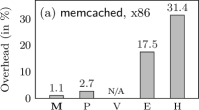
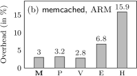
Fig. 18: Runtime overheads due to inserted fences in memcached for each strategy

debian ​​​

gathers $374$ executables. These are a subset of the goto-programs that have been built from packages of Debian Linux 7.1 by Michael Tautschnig. A small excerpt of our results is given in Fig. 17. The full data set, including a comparison with the methods from Sec. 2, is provided at http://www.cprover.org/wmm/musketeer. For each program, we give the lines of code and number of nodes in the aeg. We used musketeer on these programs to demonstrate its scalability and its ability to handle deployed code. Most programs already contain fences or operations that imply them, such as compare-and-swaps or locks. Our tool musketeer takes these fences into account and infers a set of additional fences sufficient to guarantee SC. The largest program we handle is memcached ($\sim 10000$ LoC). Our tool needs $13.9\,s$ to place fences for TSO, and $89.9\,s$ for Power. A more meaningful measure for the hardness of an instance is the number of nodes in the aeg. For example, ptunnel has 1867 nodes and 1249 LoC. The fencing takes $95.0\,s$ for TSO, but times out for Power due to the number of cycles. Not all fences inferred by musketeer are necessary to enforce SC, due to the imprecision introduced by the aeg abstraction. However, as Section 2 shows, the execution time overhead of the program versions with fences inserted by musketeer is still very low.

7.3 Impact on runtime

We finally measure the impact of fences for the program memcached, running experiments that are similar to those in Sec. 2. We built new versions of memcached according to the fencing strategies described in Sec. 2. We used in particular the memtier benchmarking tool to generate a workload for the memcached daemon, and killed the daemon after $60\,s$. Fig. 1 shows the mean overhead w.r.t. the original, unmodified program.

Unsurprisingly, adding a fence after every access to static or heap data has a significant performance effect. Similarly, adding fences via an escape analysis is expensive, yielding overheads of up to 17.5 %. Amongst the approaches guaranteeing SC (i.e. all but v), the best results were achieved with our tool musketeer. We again computed the confidence intervals to check the statistical significance in Fig. 19.

	stack on x86	stack on ARM	queue on x86	queue on ARM
(o)	[9.757; 9.798]	[11.291; 11.369]	[11.947; 11.978]	[20.441; 20.634]
(m)	[9.818; 9.850]	[11.316; 11.408]	[12.067; 12.099]	[20.687; 20.857]
(p)	[10.077; 10.155]	[11.995; 12.109]	[13.339; 13.373]	[22.035; 22.240]
(v)	N/A	[11.779; 11.834]	N/A	[21.334; 21.526]
(e)	[11.316; 11.360]	[13.071; 13.200]	[13.949, 13.981]	[22.722; 22.903]
(h)	[12.286; 12.325]	[14.676; 14.844]	[14.941, 14.963]	[25.468; 25.633]

Fig. 19: Confidence intervals for data structure experiments

8 Conclusion

We introduced a novel method for deriving a set of fences, which we implemented in a new tool called musketeer. We compared it to existing tools and observed that it outperforms them. We demonstrated on our debian series that musketeer can handle deployed code, with a large potential for scalability.

Acknowledgements

We thank Michael Tautschnig for the Debian binaries, Mohamed Faouzi Atig, Egor Derevenetc, Carsten Fuhs, Alexander Linden, Roland Meyer, Tyler Sorensen, Martin Vechev, Eran Yahav and our reviewers for their feedback. We thank Alexander Linden and Martin Vechev again for giving us access to their tools.

References

- [AAC+13] Parosh Aziz Abdulla, Mohamed Faouzi Atig, Yu-Fang Chen, Carl Leonardsson, and Ahmed Rezine, Memorax, a precise and sound tool for automatic fence insertion under TSO, Tools and Algorithms for the Construction and Analysis of Systems (TACAS), LNCS, Springer, 2013, pp. 530–536.
- [AG95] S. V. Adve and K. Gharachorloo, Shared memory consistency models: A tutorial, IEEE Computer 29 (1995), no. 12, 66–76.
- [AKL+11] Jade Alglave, Daniel Kroening, John Lugton, Vincent Nimal, and Michael Tautschnig, Soundness of data flow analyses for weak memory models, Programming Languages and Systems (APLAS), LNCS, vol. 7078, Springer, 2011, pp. 272–288.
- [AKNT13] Jade Alglave, Daniel Kroening, Vincent Nimal, and Michael Tautschnig, Software verification for weak memory via program transformation, European Symposium on Programming (ESOP), 2013.
- [AM11] J. Alglave and L. Maranget, Stability in weak memory models, Computer Aided Verification (CAV), LNCS, vol. 6806, Springer, 2011, pp. 50–66.
- [AMSS10] J. Alglave, L. Maranget, S. Sarkar, and P. Sewell, Fences in weak memory models, Computer Aided Verification (CAV), LNCS, vol. 6174, Springer, 2010, pp. 258–272.
- [BDM13] Ahmed Bouajjani, Egor Derevenetc, and Roland Meyer, Checking and enforcing robustness against TSO, European Symposium on Programming (ESOP), LNCS, vol. 7792, Springer, 2013, pp. 533–553.
- [BMM11] A. Bouajjani, R. Meyer, and E. Moehlmann, Deciding robustness against total store ordering, Automata, Languages and Programming (ICALP), LNCS, vol. 6756, Springer, 2011, pp. 428–440.
- [c1111] Information technology – Programming languages – C, BS ISO/IEC 9899:2011, 2011.
- [CL05] David Chase and Yossi Lev, Dynamic circular work-stealing deque, SPAA, ACM, 2005, pp. 21–28.
- [DFG+00] David Detlefs, Christine H. Flood, Alex Garthwaite, Paul A. Martin, Nir Shavit, and Guy L. Steele Jr., Even better DCAS-based concurrent deques, Distributed Computing (DISC), LNCS, vol. 1914, Springer, 2000, pp. 59–73.
- [Dic09] David Dice, November 2009.
- [Dij65] Edsger W. Dijkstra, Solution of a problem in concurrent programming control, Commun. ACM 8 (1965), no. 9, 569.
- [FLM03] Xing Fang, Jaejin Lee, and Samuel P. Midkiff, Automatic fence insertion for shared memory multiprocessing, International Conference on Supercomputing (ICS), ACM, 2003, pp. 285–294.
- [FLR98] Matteo Frigo, Charles E. Leiserson, and Keith H. Randall, The implementation of the Cilk-5 multithreaded language, PLDI, ACM, 1998, pp. 212–223.
- [KSKZ09] Vineet Kahlon, Nishant Sinha, Erik Kruus, and Yun Zhang, Static data race detection for concurrent programs with asynchronous calls, FSE, 2009.
- [KVY10] Michael Kuperstein, Martin T. Vechev, and Eran Yahav, Automatic inference of memory fences, Formal Methods in Computer-Aided Design (FMCAD), IEEE, 2010, pp. 111–119.
- [KVY11] , Partial-coherence abstractions for relaxed memory models, PLDI, 2011, pp. 187–198.
- [KY96] Arvind Krishnamurthy and Katherine A. Yelick, Analyses and optimizations for shared address space programs, J. Par. Dist. Comp. 38 (1996), no. 2.
- [Lam79] L. Lamport, How to Make a Correct Multiprocess Program Execute Correctly on a Multiprocessor, IEEE Trans. Comput. 46 (1979), no. 7.
- [Lam87] Leslie Lamport, A fast mutual exclusion algorithm, ACM Trans. Comput. Syst. 5 (1987), no. 1.
- [LNP+12] Feng Liu, Nayden Nedev, Nedyalko Prisadnikov, Martin T. Vechev, and Eran Yahav, Dynamic synthesis for relaxed memory models, PLDI, ACM, 2012, pp. 429–440.
- [LP01] J. Lee and D.A. Padua, Hiding relaxed memory consistency with a compiler, IEEE Transactions on Computers 50 (2001), 824–833.
- [LW13] Alexander Linden and Pierre Wolper, A verification-based approach to memory fence insertion in PSO memory systems, Tools and Algorithms for the Construction and Analysis of Systems (TACAS), LNCS, vol. 7795, Springer, 2013, pp. 339–353.
- [MSM+11] Daniel Marino, Abhayendra Singh, Todd D. Millstein, Madanlal Musuvathi, and Satish Narayanasamy, A case for an SC-preserving compiler, PLDI, ACM, 2011, pp. 199–210.
- [MVS09] Maged M. Michael, Martin T. Vechev, and Vijay A. Saraswat, Idempotent work stealing, Principles and Practice of Parallel Programming (PPOPP), ACM, 2009, pp. 45–54.
- [ND13] Brian Norris and Brian Demsky, CDSchecker: checking concurrent data structures written with C/C++ atomics, Object Oriented Programming Systems Languages & Applications (OOPSLA), 2013, pp. 131–150.
- [OSS09] S. Owens, S. Sarkar, and P. Sewell, A better x86 memory model: x86-TSO, Theorem Proving in Higher Order Logics (TPHOLs), LNCS, vol. 5674, Springer, 2009, pp. 391–407.
- [Pet81] Gary L. Peterson, Myths about the mutual exclusion problem, Inf. Process. Lett. 12 (1981), no. 3, 115–116.
- [ppc09] Power isa version 2.06, 2009.
- [SFW+05] Zehra Sura, Xing Fang, Chi-Leung Wong, Samuel P. Midkiff, Jaejin Lee, and David A. Padua, Compiler techniques for high performance sequentially consistent Java programs, PPOPP, ACM, 2005, pp. 2–13.
- [spa94] Sparc Architecture Manual Version 9, 1994.
- [SS88] D. Shasha and M. Snir, Efficient and correct execution of parallel programs that share memory, TOPLAS 10 (1988), no. 2, 282–312.
- [Szy88] Boleslaw K. Szymanski, A simple solution to Lamport’s concurrent programming problem with linear wait, ICS, 1988, pp. 621–626.
- [Tar73] R. Tarjan, Enumeration of the elementary circuits of a directed graph, SIAM J. Comput. 2 (1973), no. 3, 211–216.
- [VZN11] Viktor Vafeiadis and Francesco Zappa Nardelli, Verifying fence elimination optimisations, Static Analysis (SAS), LNCS, vol. 6887, Springer, 2011, pp. 146–162.