Absolute properties of the eclipsing binary system AQ Serpentis: A stringent test of convective core overshooting in stellar evolution models

Abstract

We report differential photometric observations and radial-velocity measurements of the detached, 1.69-day period, double-lined eclipsing binary AQ Ser. Accurate masses and radii for the components are determined to better than 1.8% and 1.1%, respectively, and are $M_{1}=1.417\pm 0.021\,M_{\sun}$, $M_{2}=1.346\pm 0.024\,M_{\sun}$, $R_{1}=2.451\pm 0.027\,R_{\sun}$, and $R_{2}=2.281\pm 0.014\,R_{\sun}$. The temperatures are $6340\pm 100$ K (spectral type F6) and $6430\pm 100$ K (F5), respectively. Both stars are considerably evolved, such that predictions from stellar evolution theory are particularly sensitive to the degree of extra mixing above the convective core (overshoot). The component masses are different enough to exclude a location in the H-R diagram past the point of central hydrogen exhaustion, which implies the need for extra mixing. Moreover, we find that current main-sequence models are unable to match the observed properties at a single age even when allowing the unknown metallicity, mixing length parameter, and convective overshooting parameter to vary freely and independently for the two components. The age of the more massive star appears systematically younger. AQ Ser and other similarly evolved eclipsing binaries showing the same discrepancy highlight an outstanding and largely overlooked problem with the description of overshooting in current stellar theory.

1. Introduction

The eclipsing binary AQ Ser (GSC 00340-00588, BD+03 3015, $V=10.58$) was discovered as a variable star by Hoffmeister (1935). Its correct period of 1.6874 days and eclipse ephemeris were determined much later by Soloviev (1951). The light curve shows relatively deep (0.6 mag) and nearly identical primary and secondary eclipses, and the spectral types of the stars have been reported as F5 and A2 (Hill et al., 1975), although the latter classification for the less massive star is probably too early. The system has been little studied since its discovery, other than the occasional measurement of times of eclipse.

The main motivation for this work is to present new photometric and spectroscopic observations of AQ Ser, with which we determine for the first time accurate absolute dimensions for the system and establish the evolutionary status of the stars. Both components appear to be at the very end of their hydrogen-burning phase, a location of the H-R diagram in which only a few other well-measured eclipsing binaries are found. The predicted properties of such stars from stellar evolution theory are especially sensitive to the degree of convective core overshooting adopted in the models, and a previous study by Clausen et al. (2010) has highlighted the difficulties that current models appear to have in reproducing the stellar properties of both components at a single age. The newly determined absolute dimensions for AQ Ser allow us an opportunity to revisit this problem here.

2. Observations and Reductions

2.1. Differential photometry

Photometric measurements of AQ Ser were determined by two different and independent robotic observatories: the URSA WebScope, and the NFO WebScope. The URSA WebScope uses a 10-inch Meade LX200 SCT telescope with an SBIG ST8 CCD camera, housed in a Technical Innovations RoboDome on the roof of the Kimpel Hall on the University of Arkansas campus at Fayetteville, and is controlled by an Apple Macintosh G4 computer in a nearby control room. The field of view is about 20$\times$30 arc minutes. Observations with a Bessel $V$ filter were carried out from 2003 June to 2011 July, producing a total of 8642 science frames from 80-second exposures. The two comparison stars for AQ Ser (‘var’), both within 8 arc minutes of the variable star, were GSC 00340-00252 (‘comp’; $V=10.99$, G5 V) and GSC 00341-00211 (‘ck’; $V=11.60$, G2 V). It was eventually found that the ck star is a low-amplitude variable with a sinusoidal variation of half-amplitude 0.017 mag and a period of about four years. Differential magnitudes in this study were therefore based on the var$-$comp magnitudes only.

The NFO WebScope is located near Silver City (NM) in a roll-off roof structure, and consists of a 24-inch Cassegrain reflector with a field-widening correcting lens near the focus (see Grauer et al., 2008). At the focus is a camera based on the Kodak KAF-4301E CCD chip, with a field of view of about 27$\times$27 arc minutes. AQ Ser was observed at the NFO between 2005 January and 2007 June, producing a total of 6694 observations from 80-second exposures with a Bessel $V$ filter.

All images were measured using a computer application (Measure) that matched a pattern file with the image, and then determined the differential magnitude after correction for dark current, sky brightness, and responsivity variations across the field of view.

As we have noted in the past (e.g., Sandberg Lacy et al., 2008), the telescopes we used in this study produce systematic shifts of a few hundredths of a magnitude in the photometric zero point from night to night, and in the case of the NFO WebScope, from one side of the German equatorial mount axis to the other. The shifts are very much less for the URSA WebScope than for the NFO, which shows that this is an effect of the optical system being used, and is not intrinsic to the stars themselves. The offsets are due to a non-uniform responsivity across the field of view, combined with imprecise centering from night to night. In the case of the NFO, we removed most of this effect by using dithered exposures of open clusters to fit a 2-D polynomial function to the responsivity variations, resulting in a photometric flat that is included in the initial data reduction procedures. Residual offsets remaining after this process were then removed by using an initial photometric orbital fit model (see Sect. 4) to determine the values of the nightly offsets and to remove them from the data. In this case, 130 nightly shifts were removed from the URSA data, and 197 shifts were removed from the NFO data. The typical precision of the final AQ Ser data sets is about 9 mmag for URSA and 5 mmag for NFO. The measurements including nightly corrections are listed in Table 1 (URSA) and Table 2 (NFO).

Table 1Differential $V$-band measurements of AQ Ser from the URSA WebScope.

HJD	Orbital	$\Delta V$
($2,\!400,\!000+$)	phase	(mag)
52814.60641	0.0963	$-$0.366
52814.60833	0.0975	$-$0.396
52814.61022	0.0986	$-$0.365
52814.61212	0.0997	$-$0.366
52814.61399	0.1008	$-$0.375

Note. — Orbital phase is computed with the ephemeris in Sect. 3. Table 1 is published in its entirety in the electronic edition of the journal. A portion is shown here for guidance regarding its form and content.

Table 2Differential $V$-band measurements of AQ Ser from the NFO WebScope.

HJD	Orbital	$\Delta V$
($2,\!400,\!000+$)	phase	(mag)
53377.03321	0.4000	$-$0.390
53377.03484	0.4010	$-$0.390
53377.03647	0.4019	$-$0.390
53377.03806	0.4029	$-$0.390
53377.03970	0.4038	$-$0.386

Note. — Orbital phase is computed with the ephemeris in Sect. 3. Table 2 is published in its entirety in the electronic edition of the journal. A portion is shown here for guidance regarding its form and content.

2.2. Spectroscopy

Spectroscopic observations of AQ Ser were carried out at the Harvard-Smithsonian Center for Astrophysics using an echelle spectrograph on the 1.5-m Tillinghast reflector at the F.L. Whipple Observatory (Mount Hopkins, AZ). A single echelle order 45 Å wide was recorded with an intensified photon-counting Reticon detector, at a central wavelength near 5190 Å that includes the Mg I b triplet. The resolving power of these observations is $\lambda/\Delta\lambda\approx 35,\!000$. We gathered 39 spectra between 2004 March and 2008 June, with signal-to-noise ratios ranging between 22 and 41 per resolution element of 8.5 km s^-1.

All our spectra appear double-lined. Radial velocities were obtained using the two-dimensional cross-correlation technique TODCOR (Zucker & Mazeh, 1994), with templates chosen from a large library of calculated spectra based on model atmospheres by R. L. Kurucz (see Nordström et al., 1994; Latham et al., 2002). The four main parameters of the templates are the effective temperature $T_{\rm eff}$, rotational velocity ($v\sin i$ when seen in projection), metallicity [m/H], and surface gravity $\log g$. The ones affecting the velocities the most are $T_{\rm eff}$ and $v\sin i$. Consequently, we held $\log g$ fixed at values of 4.0 for both stars, which is near the final values reported below in Sect. 5, and we assumed solar metallicity. The optimum $T_{\rm eff}$ and $v\sin i$ values were determined by running grids of cross-correlations, seeking the maximum of the correlation coefficient averaged over all exposures and weighted by the strength of each spectrum (see Torres et al., 2002). The rotational velocities we obtained are $v\sin i=59\pm 10\,{\rm km\thinspace s^{-1}}$ for the hotter and less massive star (hereafter star A) and $v\sin i=73\pm 10\,{\rm km\thinspace s^{-1}}$ for the cooler one (star B). The significant rotational line broadening in both stars and the relatively low signal-to-noise ratios cause the uncertainties above to be fairly large, and also prevent us from establishing the temperatures accurately. Only a rough estimate of $T_{\rm eff}$ could be obtained. The values adopted from our analysis in Sect. 5 are $T_{\rm eff}=6430$ K for the less massive component and $T_{\rm eff}=6340$ K for the other. The uncertainty in these values has little effect on the velocities.

We also determined the light ratio at the mean wavelength of our observations (which is close to the $V$ band), following the prescription by Zucker & Mazeh (1994). We obtained $\ell_{\rm B}/\ell_{\rm A}=1.05\pm 0.04$, formally indicating that the cooler and more massive star of the system is visually the brightest.

As in previous studies using similar spectroscopic material, we made an assessment of potential systematic errors in our radial velocities that may result from residual line blending as well as lines shifting in and out of our narrow spectral window as a function of orbital phase (see Latham et al., 1996). We did this by performing numerical simulations analogous to those described by Torres et al. (1997), and we applied corrections to the raw velocities based on these simulations to mitigate the effect. The corrections were typically less than 2.5 km s^-1 for the hotter star and less than 2 km s^-1 for the cooler star, which are smaller than our internal velocity errors ($\sim$5 km s^-1). The effect of these corrections on the absolute masses is minimal.

Finally, the stability of the zero-point of our velocity system was monitored by taking nightly exposures of the dusk and dawn sky, and small run-to-run corrections (typically under 1 km s^-1) were applied to the velocities as described by Latham (1992). The adopted heliocentric velocities including all corrections are listed in Table 3, together with their uncertainties and the residuals from our adopted orbital solution described below.

Table 3Heliocentric radial velocities for AQ Ser.

HJD	Orbital	RVA	RVB	$(O\!-\!C)_{\rm A}$	$(O\!-\!C)_{\rm B}$
($2,\!400,\!000+$)	phase	(km s-1)	(km s-1)	(km s-1)	(km s-1)
53073.9118	0.7651	$158.1\pm 4.6$	$-106.9\pm 5.9$	$10.8$	$-7.2$
53096.9083	0.3932	$-62.0\pm 4.2$	$90.6\pm 5.3$	$-3.4$	$-5.0$
53103.9912	0.5907	$87.1\pm 4.8$	$-36.6\pm 6.2$	$-2.2$	$8.0$
53126.9531	0.1983	$-103.8\pm 3.8$	$128.5\pm 4.8$	$-3.8$	$-6.6$
53133.8183	0.2667	$-110.8\pm 4.2$	$153.4\pm 5.4$	$-4.8$	$12.7$
53154.8085	0.7059	$142.7\pm 3.5$	$-101.2\pm 4.4$	$-0.2$	$-5.6$
53155.7765	0.2795	$-105.8\pm 3.3$	$135.4\pm 4.2$	$-1.2$	$-4.0$
53160.7788	0.2440	$-104.6\pm 4.8$	$147.3\pm 6.0$	$2.0$	$6.0$
53161.7409	0.8141	$141.8\pm 4.6$	$-97.0\pm 5.9$	$4.1$	$-6.4$
53182.7419	0.2597	$-109.3\pm 5.2$	$141.0\pm 6.6$	$-2.9$	$-0.2$
53188.6973	0.7889	$140.4\pm 3.1$	$-90.3\pm 3.9$	$-3.7$	$6.4$
53192.7251	0.1759	$-88.6\pm 5.0$	$137.3\pm 6.4$	$4.5$	$8.8$
53452.8657	0.3396	$-84.2\pm 4.8$	$126.3\pm 6.0$	$2.9$	$3.6$
53455.9574	0.1718	$-96.9\pm 5.2$	$122.6\pm 6.6$	$-5.2$	$-4.5$
53456.9539	0.7624	$152.4\pm 5.1$	$-101.0\pm 6.5$	$4.9$	$-1.2$
53483.8617	0.7084	$136.2\pm 4.6$	$-100.5\pm 5.9$	$-7.3$	$-4.4$
53488.8435	0.6607	$127.1\pm 3.8$	$-72.0\pm 4.8$	$-1.2$	$9.7$
53543.7496	0.1990	$-105.0\pm 4.8$	$133.5\pm 6.1$	$-4.8$	$-1.7$
53576.7161	0.7355	$152.8\pm 5.0$	$-97.1\pm 6.4$	$5.5$	$2.6$
53866.8395	0.6675	$129.1\pm 5.1$	$-85.0\pm 6.4$	$-2.1$	$-0.6$
53872.8047	0.2026	$-87.0\pm 5.0$	$125.4\pm 6.4$	$14.1$	$-10.7$
53873.7141	0.7415	$145.0\pm 4.6$	$-99.6\pm 5.9$	$-2.6$	$0.5$
53895.7489	0.7997	$138.6\pm 4.6$	$-91.5\pm 5.8$	$-3.0$	$2.9$
53901.6867	0.3186	$-94.6\pm 5.3$	$127.6\pm 6.7$	$0.4$	$-2.7$
54137.0002	0.7693	$150.5\pm 5.1$	$-97.7\pm 6.4$	$3.6$	$1.7$
54158.9724	0.7904	$139.8\pm 5.7$	$-94.1\pm 7.2$	$-4.0$	$2.3$
54162.9989	0.1766	$-93.7\pm 5.2$	$138.2\pm 6.6$	$-0.3$	$9.5$
54191.9366	0.3256	$-100.9\pm 4.8$	$126.6\pm 6.1$	$-8.3$	$-1.4$
54217.8096	0.6584	$126.1\pm 5.2$	$-84.3\pm 6.6$	$-1.2$	$-3.5$
54224.8170	0.8111	$142.7\pm 4.9$	$-90.4\pm 6.2$	$4.1$	$1.1$
54250.7786	0.1963	$-98.8\pm 5.2$	$132.0\pm 6.6$	$0.7$	$-2.6$
54514.0334	0.2056	$-99.5\pm 5.2$	$139.2\pm 6.6$	$2.3$	$2.4$
54520.9910	0.3288	$-88.4\pm 4.8$	$123.2\pm 6.1$	$3.0$	$-3.7$
54546.9391	0.7061	$142.6\pm 5.0$	$-102.2\pm 6.4$	$-0.5$	$-6.6$
54574.9033	0.2781	$-99.5\pm 4.7$	$145.1\pm 6.0$	$5.2$	$5.6$
54578.8906	0.6411	$114.6\pm 4.4$	$-78.2\pm 5.6$	$-4.6$	$-5.2$
54579.8440	0.2061	$-96.5\pm 4.7$	$140.3\pm 5.9$	$5.4$	$3.5$
54602.7922	0.8056	$142.7\pm 4.9$	$-85.6\pm 6.2$	$2.6$	$7.3$
54633.7734	0.1656	$-91.6\pm 5.2$	$124.1\pm 6.6$	$-2.4$	$-0.6$

A spectroscopic orbit was derived from these measurements with the orbital period and epoch of the photometric primary eclipse held fixed at their values determined in Sect. 3. Fits allowing for a non-zero eccentricity resulted in a value not significantly different from zero. Consequently for the final solution we adopted a circular orbit. The elements we obtained are listed in Table 4, and the observations along with this fit are displayed in Figure 1.

Table 4Spectroscopic orbital solution for AQ Ser.

Parameter	Value
Orbital elements
$P$ (days)	1.68743059
${\rm Min~{}I}$ (HJD$-$2,400,000)	53,399.982270
$\gamma$ (km s-1)	+20.58 $\pm$ 0.58+0
$K_{\rm A}$ (km s-1)	127.27 $\pm$ 0.8000
$K_{\rm B}$ (km s-1)	120.8 $\pm$ 1.000
$e$	0.0 (fixed)
Derived quantities
$M_{\rm A}\sin^{3}i$ ($M_{\sun}$)	1.300 $\pm$ 0.023
$M_{\rm B}\sin^{3}i$ ($M_{\sun}$)	1.369 $\pm$ 0.021
$q\equiv M_{\rm B}/M_{\rm A}$	1.054 $\pm$ 0.011
$a_{\rm A}\sin i$ (106 km)	2.953 $\pm$ 0.018
$a_{\rm B}\sin i$ (106 km)	2.803 $\pm$ 0.023
$a\sin i$ ($R_{\sun}$)	8.274 $\pm$ 0.043
Other quantities pertaining to the fit
$N_{\rm obs}$	39
Time span (days)	1559.9
$\sigma_{\rm A}$ (km s-1)	4.6
$\sigma_{\rm B}$ (km s-1)	5.9

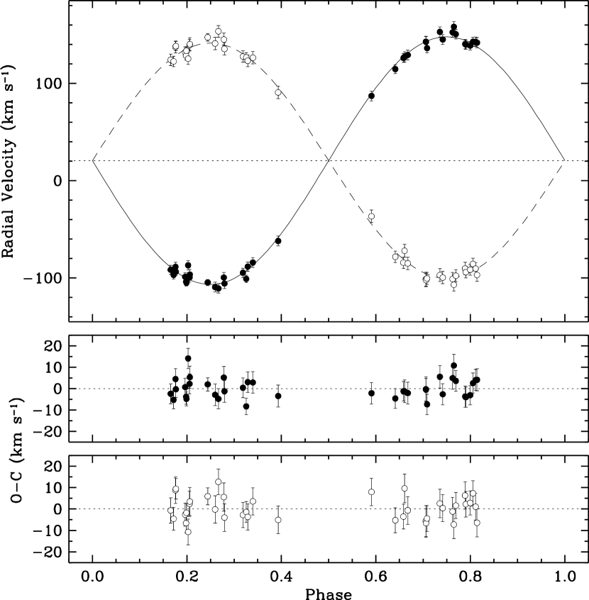
Figure 1.— Top: Measured radial velocities for AQ Ser along with our best-fit orbit model. Solid circles correspond to the photometric primary (hotter and less massive star), and open circles to the secondary. The horizontal dotted line represents the center-of-mass velocity. Phase 0.0 corresponds to the eclipse of the hotter component. Bottom: $O-C$ residuals from the best orbital fit (same symbols as above).

3. Ephemeris

A total of 48 times of eclipse for AQ Ser were gathered from the literature, and were obtained by photographic, visual, photoelectric, or CCD techniques. From the 27 photoelectric/CCD measurements we determined a preliminary ephemeris, and detected no significant trends indicative of any period changes in the $O\!-\!C$ residuals. A large number of additional timing measurements (167 in total) were derived from our own URSA and NFO differential photometry described previously. Of these, 39 timings are based on eclipse events with reasonably good coverage, i.e., with observations on both the ascending and descending branches of the primary or secondary minima. These were measured using either the traditional Kwee & van Woerden (1956) method (KvW) or a parabolic fit, or with an alternate technique relying on fitting a synthetic light-curve model to the observations, with the model being computed using the Wilson-Devinney code (WD; Wilson & Devinney, 1971) and subsequent improvements by Vaz et al. (2007) pertaining to the ephemeris determination. For the latter method we held all light-curve parameters fixed to values close to our final solutions reported later, and adjusted only the time of eclipse. The results from these three procedures were then weight-averaged (see below). We considered measurements from URSA and NFO separately. For the 128 URSA/NFO eclipses with only partial coverage, many having observations on only one of the branches, we first predicted the approximate center of the event using the preliminary ephemeris above, and then adjusted this value using the WD modeling just described.

Realistic uncertainties for these eclipse timings are not easy to establish, and can depend not only on the quality of the measurements, but also in our case on the method used to determine them. We proceeded as follows. We initially considered the uncertainties from our own measurements to be equal to the internal errors from each method, and solved for a linear ephemeris adjusting (scaling) these uncertainties by iterations so as to achieve reduced $\chi^{2}$ values near unity. This was done separately by method (KvW, parabolic, or WD fits), telescope (URSA, NFO), and binary component (primary, secondary), twelve groups in all. Similarly, for the measurements from the literature we considered the photographic and visual timings together as a group, and the CCD and photoelectric timings as another, separately for the primary and secondary. For the final fit, minima measured from our URSA or NFO data by more than one method were merged together into weighted averages with corresponding uncertainties. All 215 timings (124 for the primary eclipse, 91 for the secondary) are reported in Table 5 along with their final, rescaled errors. The resulting linear ephemeris (HJD) is

$${\rm Min~{}I}=2,\!453,\!399.982270(47)+1.68743059(17)E~{},$$ (1)

with the figures in parentheses representing uncertainties in units of the last significant digit. Residuals from the above fit are listed in Table 5, and show no obvious pattern as a function of time. Using only the secondary timings we find a mean phase for the secondary eclipse of $0.50010\pm 0.00008$. This is consistent with 0.5, supporting our assumption of a circular orbit in our analysis below.

Table 5Eclipse timing measurements for AQ Ser.

HJD	Type	Source	$O\!-\!C$
($2,\!400,\!000+$)			(days)
28333.220(35)	p	P	$0.0192$
28371.154(19)	s	P	$-0.0140$
28655.561(35)	p	P	$0.0609$
28661.408(19)	s	P	$0.0019$
28679.129(105)	p	P	$0.0049$

Note. — Table 5 is published in its entirety in the electronic edition of the journal. A portion is shown here for guidance regarding its form and content.

4. Light curve solutions

The light curves of AQ Ser show moderate proximity effects, with the curvature between the minima being mostly due to the deformation of the components and, to a smaller degree, to the mutual illumination. The small but significant difference in depth between the primary and secondary eclipses indicates a slightly cooler temperature for the secondary star, which in this case corresponds to the more massive and presumably more evolved component.

The analysis of the differential photometry of AQ Ser was carried out using a version of the WD model (Wilson & Devinney, 1971; Wilson, 1979, 1993) extensively improved as described by Vaz et al. (2007) and references therein. The URSA and NFO light curves were modeled both separately and together, adopting the ephemeris in Eq.(1). The orbit was assumed to be circular, based on the evidence from the eclipse timings presented above and from the spectroscopic analysis. The main quantities we adjusted are the orbital inclination angle, $i$, the temperature of the secondary, $T_{\rm eff}^{\rm B}$, the gravitational pseudo-potentials, $\Omega$, an arbitrary phase shift, $\Delta\phi$, and a luminosity normalization factor. The primary temperature was held fixed at the value $T_{\rm eff}^{\rm A}=6430$ K described in Sect. 5, and the mass ratio was fixed at the value listed in Table 4. Because the orbital period is short, we assumed both components have their rotation synchronized with the orbital motion. For the bolometric reflection albedos, $A$, we explored two different treatments: in one we held them fixed at the value of 0.5 appropriate for stars with convective envelopes such as these, and in the other we allowed them to vary freely as the iterations proceeded. The gravity-brightening exponents $\beta$ were computed using the local value of $T_{\rm eff}$ for each point on the stellar surfaces, taking into account mutual illumination following Alencar & Vaz (1997) and Alencar et al. (1999). The radiated flux of both components was described using the PHOENIX atmosphere models (Allard & Hauschildt, 1995; Allard et al., 1997; Hauschildt et al., 1997a, b). The luminosity of the secondary was calculated internally from its size and $T_{\rm eff}$. All solutions were performed by alternating between the least-squares and simplex methods to improve convergence (see, e.g., Press et al., 1992), with equal weights for all measurements. Iterations were stopped when the corrections to the individual elements were at least one order of magnitude smaller than the formal errors, and they oscillated between positive and negative in consecutive iterations.

Table 6Light-curve solutions for AQ Ser to explore different limb-darkening laws and different treatments of the reflection albedos.

$i~{}(^{\circ})$	$T_{\rm eff}^{\rm{B}}$ (K)	$A_{\rm A}$	$A_{\rm B}$	$\Omega_{\rm A}$	$\Omega_{\rm B}$	$\Delta\phi$	${\sigma{\rm(mmag)}}\atop{\scriptscriptstyle\mathrm{URSA\,{\displaystyle/}\,NFO}}$
LINEAR limb darkening law
81.2553	6347.78	0.5000	0.5000	4.7765	4.6224	1.18	9.015 / 5.487
$\pm 52$	$\pm 66$	fixed	fixed	$\pm 14$	$\pm 11$	$\pm 10$
81.3235	6343.17	0.4216	0.3972	4.7777	4.6358	1.21	9.010 / 5.460
$\pm 76$	$\pm 72$	$\pm 79$	$\pm 73$	$\pm 16$	$\pm 13$	$\pm 12$
LOGARITHMIC limb darkening law
81.3498	6346.82	0.5000	0.5000	4.7659	4.6307	1.15	9.034 / 5.507
$\pm 51$	$\pm 66$	fixed	fixed	$\pm 14$	$\pm 12$	$\pm 10$
81.4415	6341.77	0.4028	0.3762	4.7664	4.6496	1.19	9.016 / 5.482
$\pm 77$	$\pm 71$	$\pm 82$	$\pm 75$	$\pm 15$	$\pm 15$	$\pm 10$
SQUARE ROOT limb darkening law
81.3362	6342.54	0.5000	0.5000	4.7665	4.6291	1.14	9.033 / 5.508
$\pm 51$	$\pm 66$	fixed	fixed	$\pm 14$	$\pm 12$	$\pm 10$
81.4319	6337.35	0.4006	0.3722	4.7673	4.6482	1.20	9.017 / 5.477
$\pm 79$	$\pm 71$	$\pm 82$	$\pm 74$	$\pm 16$	$\pm 14$	$\pm 10$
QUADRATIC limb darkening law
81.3352	6341.43	0.5000	0.5000	4.7663	4.6301	1.15	9.026 / 5.498
$\pm 51$	$\pm 66$	fixed	fixed	$\pm 14$	$\pm 12$	$\pm 10$
81.4231	6336.75	0.4119	0.3855	4.7671	4.6479	1.20	9.016 / 5.474
$\pm 79$	$\pm 71$	$\pm 81$	$\pm 74$	$\pm 16$	$\pm 15$	$\pm 10$

Note. — Test solutions for a fixed mass ratio of $q\equiv M_{\rm B}/M_{\rm A}=1.054\pm 0.011$ (Sect. 2.2). Phase shifts $\Delta\phi$ are in units of $10^{-4}P$. Uncertainties are given in units of the last significant digit and represent internal errors from the WD code.

Four different limb-darkening laws were investigated: linear, quadratic, square-root, and logarithmic (see Claret, 2000). The coefficients for these laws were interpolated from the tables by the above author using a bilinear scheme for the current values of $T_{\rm eff}$ and $\log g$ at each iteration. The results of our initial exploration of the limb-darkening laws are presented in Table 6, in which we used the URSA and NFO data simultaneously. These tests were run both holding the reflection albedos fixed, and allowing them to vary.

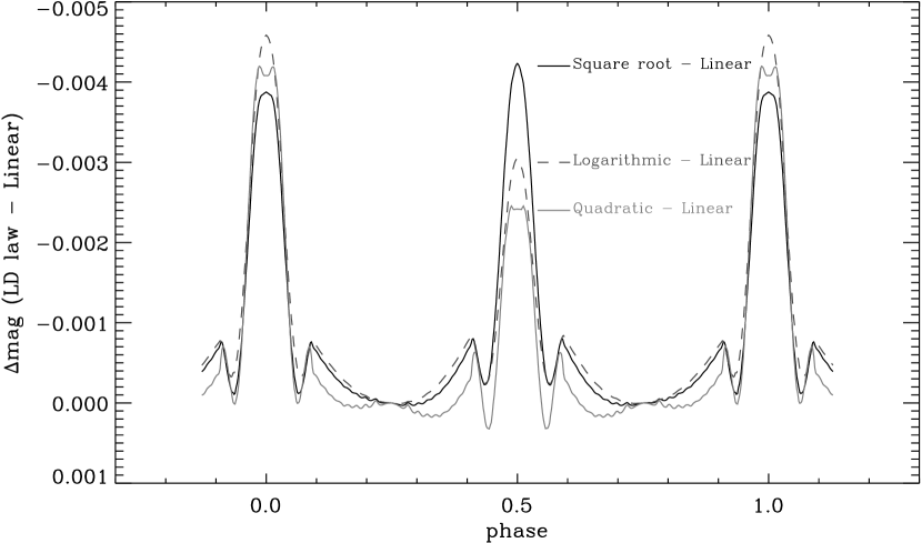
Figure 2.— Differences between light curve models that use a non-linear limb darkening law and one that adopts the linear law. The linear law results in brighter stars (deeper minima). The logarithmic and quadratic laws are the most similar to each other. The maximum amplitude of the differences compared to the linear law is only $\sim$5 mmag.

Despite the larger freedom of the model when using non-linear limb-darkening laws, we found that there is relatively little difference in the quality of the fits, and that the linear law gives marginally better solutions. Figure 2 illustrates the effect that the non-linear limb-darkening laws have on the light curves, relative to the effect of the linear law. The maximum difference for a system such as AQ Ser turns out to be quite small ($\sim$5 mmag), which explains why the resulting light elements in Table 6 are rather similar for the various laws. We also note a modest improvement in the solutions when adjusting the bolometric albedos, as opposed to leaving them fixed. The resulting values of $\beta$ are somewhat smaller than the canonical values. Based on these tests, for the final solutions we chose to adopt the linear limb-darkening law and to allow the albedos to be adjusted.

Figure 3.— Differential photometry of AQ Ser from the URSA and NFO telescopes, along with the fitted model. Phase 0.0 corresponds to the eclipse of the hotter, smaller, and less massive component. The light curves are shifted vertically for clarity. The lower panels show the $O\!-\!C$ residuals, with the typical error of a single measurement indicated in the top left corner of each panel. Remaining systematic effects in the fits are very small, as shown by a boxcar smoothing of the residuals represented in the lower panels with gray lines. The box size adopted was 220 points for URSA and 180 points for NFO.

Our final results are presented in Table 7, for the individual solutions to the URSA and NFO data and also for the combined fit. The uncertainties for the individual solutions are the internal errors reported by the WD code. For the combined fit that we adopt for the remainder of the analysis we have conservatively increased the internal errors by adding in quadrature half of the difference between the parameters for the individual solutions. Also included in Table 7 are the “volume” radii $r_{\rm vol,A}$ and $r_{\rm vol,B}$, which are used in the next section to compute the absolute radii of the components.

Table 7Final light curve solutions for AQ Ser.

Parameter	URSA	NFO	Combined	Parameter	URSA	NFO	Combined
$i$ ($\arcdeg$)	81.282	81.3418	81.323	$T_{\rm eff}^{\rm B}$ (K)	6344.5	6342.46	6343.2
	$\pm 12$	$\pm 91$	$\pm 31$		$\pm 1.2$	$\pm 97$	$\pm 1.2$
$A_{\rm A}$	0.447	0.4142	0.422	$A_{\rm B}$	0.427	0.3867	0.397
	$\pm 14$	$\pm 97$	$\pm 81$		$\pm 13$	$\pm 88$	$\pm 21$
$\Omega_{\rm A}$	4.7781	4.7783	4.7777	$\Omega_{\rm B}$	4.6282	4.6389	4.6358
	$\pm 25$	$\pm 20$	$\pm 13$		$\pm 20$	$\pm 17$	$\pm 58$
$r_{\rm A,pole}$	0.26599	0.26598	0.26602	$r_{\rm B,pole}$	0.2854	0.2846	0.2848
	$\pm 91$	$\pm 88$	$\pm 85$		$\pm 27$	$\pm 26$	$\pm 26$
$r_{\rm A,point}$	0.2839	0.2838	0.2839	$r_{\rm B,point}$	0.3082	0.3070	0.3073
	$\pm 10$	$\pm 10$	$\pm 10$		$\pm 14$	$\pm 14$	$\pm 15$
$r_{\rm A,side}$	0.2714	0.27134	0.27138	$r_{\rm B,side}$	0.2922	0.2913	0.2915
	$\pm 10$	$\pm 98$	$\pm 95$		$\pm 29$	$\pm 28$	$\pm 29$
$r_{\rm A,back}$	0.2794	0.2793	0.2794	$r_{\rm B,back}$	0.3019	0.3008	0.3011
	$\pm 12$	$\pm 12$	$\pm 12$		$\pm 32$	$\pm 31$	$\pm 31$
$r_{\rm A,vol}$	0.2725	0.2725	0.27251	$r_{\rm B,vol}$	0.2934	0.2925	0.2928
	$\pm 11$	$\pm 10$	$\pm 99$		$\pm 29$	$\pm 29$	$\pm 29$
$\Delta\phi$ ($10^{-4}P$)	1.41	1.10	1.21	$\ell_{\rm B}/\ell_{\rm A}(V)$	1.094	1.086	1.088
	$\pm 18$	$\pm 13$	$\pm 10$		$\cdots$	$\cdots$	$\cdots$
$\beta_{\rm A}$	0.312	0.312	0.312	$\beta_{\rm B}$	0.320	0.320	0.320
$x_{\rm bolo,A}$	0.3887	0.3887	0.3887	$x_{\rm bolo,B}$	0.3916	0.3916	0.3916
$x_{\rm V,A}$ (URSA)	0.6748	$\cdots$	0.6748	$x_{\rm V,B}$ (URSA)	0.6772	$\cdots$	0.6773
$x_{\rm V,A}$ (NFO)	$\cdots$	0.6748	0.6748	$x_{\rm V,B}$ (NFO)	$\cdots$	0.6774	0.6773
$\sigma_{\rm URSA}$ (mmag)	9.006	$\cdots$	9.010	$\sigma_{\rm NFO}$ (mmag)	$\cdots$	5.458	5.460

Note. — The mass ratio was held fixed at its spectroscopically determined value of $q\equiv M_{\rm B}/M_{\rm A}=1.054\pm 0.011$. The uncertainties in the relative radii $r$ account for those in the pseudo-potentials and in the mass ratio. The $V$-band light ratio $\ell_{\rm B}/\ell_{\rm A}$ is calculated at phase 0.25. The bolometric and passband-specific limb darkening coefficients $x$ were adjusted during the iterations to follow the evolution of $T_{\rm eff}$ and $\log g$. The gravity-brightening coefficients $\beta$ varied over the mutually illuminated stellar surfaces, following Alencar & Vaz (1997) and Alencar et al. (1999), and the values reported above are those for the non-illuminated hemispheres. Uncertainties in the last column include a contribution from the difference between the URSA and NFO solutions.

The observations along with the fitted model are shown in Figure 3, and residuals are displayed in the lower panels. The remaining systematic effects in the light curve are very small, as illustrated by the gray curves in the lower panels representing a running mean of the residuals. There is good agreement between the $V$-band light ratio from our final combined fit ($\ell_{\rm B}/\ell_{\rm A}=1.088$) and the spectroscopic value of $\ell_{\rm B}/\ell_{\rm A}=1.05\pm 0.04$ that we reported in Sect. 2.2, which is in a passband similar to $V$. This supports the accuracy of our solution, and in particular that of the relative radii.

5. Absolute dimensions

Our spectroscopic and photometric analyses lead to the absolute masses and radii for AQ Ser reported in Table 9 below, which have relative uncertainties smaller than 1.8% and 1.1%, respectively. Given the short orbital period of the system we have assumed that each star’s rotation is synchronized with the orbital motion. Our measured $v\sin i$ values from Sect. 2.2 are indeed consistent with the expected synchronous rotational velocities listed in the table, although they do have fairly large uncertainties.

No spectroscopic determination of the metallicity is available for AQ Ser. A rough photometric estimate was derived by means of the calibration for F stars by Crawford (1975) along with the $uvby$ observations in the Strömgren system by Hilditch & Hill (1975), which, however, lack the necessary measurement of the reddening-free index $\beta$. We circumvented this by using an estimate of the interstellar reddening from dust maps following Hakkila et al. (1997), Schlegel et al. (1998), and Drimmel et al. (2003), and an approximate distance of 580 pc (see below). These three sources give $E(B-V)$ values of 0.011, 0.039, and 0.036 mag, which are insensitive to distance changes of $\pm$100 pc. We adopt the straight average of $E(B-V)=0.029\pm 0.010$. With this value and the $uvby$ photometry the metallicity inferred for AQ Ser is ${\rm[Fe/H]}\approx-0.19$.

As indicated in Sect. 2.2, the severe line broadening does not permit us to obtain reliable spectroscopic estimates of the effective temperatures of the components. A mean temperature for the system may be derived from standard photometry available in the literature, including $JH\!K_{s}$ measurements from 2MASS (Cutri et al., 2003), $V_{\rm T}$ and $B_{\rm T}$ from the Tycho-2 catalog (Høg et al., 2000), $V$ and Strömgren $b-y$ as reported by Hilditch & Hill (1975), Johnson $B$ and $V$ from the APASS catalog (Henden et al., 2012), and Johnson-Cousins $VI_{\rm C}$ photometry from the TASS catalog (Droege et al., 2006). A total of eleven, non-independent color indices were formed for which color/temperature calibrations have been established by Casagrande et al. (2010). Appropriate reddening corrections for each of the indices were applied following Cardelli et al. (1989), using the $E(B-V)$ value established above. The resulting temperatures for a metallicity of ${\rm[Fe/H]}=-0.19$ are given in Table 8, and their weighted average is $T_{\rm eff}=6380\pm 40$ K. We adopt a more conservative error for this analysis of 100 K. The metallicity dependence of the average temperature is very small: assuming solar metallicity would lower it by only 16 K. Based on this mean photometric temperature for the system and a preliminary temperature ratio from our light curve solutions, we inferred a temperature for the hotter star of $T_{\rm eff}^{\rm A}=6430\pm 100$ K, corresponding to spectral type F5. This is the value employed in our final fits described in Sect. 4. The temperature derived for the cooler star from our solutions is $T_{\rm eff}^{\rm B}=6340\pm 100$ K, which corresponds approximately to an F6 star. The two temperatures are of course highly correlated with each other, and the temperature difference is much better determined than the absolute values, as it is directly related to the well-measured difference in eclipse depths. We estimate the difference as $\Delta T_{\rm eff}=90\pm 20$ K.

Table 8Color indices and mean effective temperatures for AQ Ser.

Index	Value (mag)	$T_{\rm eff}$ (K)	Source
Johnson $B-V$	$0.481\pm 0.057$	$6388\pm 241$	1
Johnson-Cousins $V-I_{\rm C}$	$0.632\pm 0.215$	$6153\pm 542$	2
2MASS $V-J$	$0.949\pm 0.026$	$6475\pm 103$	3 , 4
2MASS $V-H$	$1.176\pm 0.025$	$6392\pm\phantom{0}77$	3 , 4
2MASS $V-K_{s}$	$1.235\pm 0.021$	$6426\pm\phantom{0}71$	3 , 4
2MASS $J-K_{s}$	$0.286\pm 0.031$	$6239\pm 210$	4
Tycho $B_{\rm T}-V_{\rm T}$	$0.556\pm 0.081$	$6288\pm 267$	5
Tycho-2MASS $V_{\rm T}-J$	$1.084\pm 0.062$	$6296\pm 169$	4 , 5
Tycho-2MASS $V_{\rm T}-H$	$1.311\pm 0.061$	$6264\pm 118$	4 , 5
Tycho-2MASS $V_{\rm T}-K_{s}$	$1.370\pm 0.060$	$6307\pm 120$	4 , 5
Strömgren $b-y$	$0.327\pm 0.030$	$6401\pm 208$	3

Note. — Sources are: 1. Henden et al. (2012); 2. Droege et al. (2006); 3. Hilditch & Hill (1975); 4. Cutri et al. (2003); 5. Høg et al. (2000). Temperature uncertainties include contributions from the photometry, reddening, and estimated systematic errors as well as the scatter in the calibrations following Casagrande et al. (2010). The metallicity adopted is ${\rm[Fe/H]}=-0.19$. In computing the temperatures all photometric indices were corrected for reddening following Cardelli et al. (1989), using $E(B-V)=0.029\pm 0.010$.

Table 9Physical properties of AQ Ser.

Parameter	Star A	Star B
Absolute dimensions
Mass ($M_{\sun}$)	1.346 $\pm$ 0.024	1.417 $\pm$ 0.022
Radius ($R_{\sun}$)	2.281 $\pm$ 0.014	2.451 $\pm$ 0.027
$\log g$ (cgs)	3.8504 $\pm$ 0.0094	3.810 $\pm$ 0.012
$v_{\rm sync}\sin i$ (km s-1)	67.6 $\pm$ 0.40	72.6 $\pm$ 0.80
$v\sin i$ (km s-1)	59 $\pm$ 10	73 $\pm$ 10
$a$ ($R_{\sun}$)	8.370 $\pm$ 0.044
Radiative and other properties
$T_{\rm eff}$ (K)	6430 $\pm$ 1000	6340 $\pm$ 1000
$\log L/L_{\sun}$	0.901 $\pm$ 0.027	0.939 $\pm$ 0.042
$M_{\rm bol}$ (mag)	2.479 $\pm$ 0.069	2.38 $\pm$ 0.10
${\rm BC}_{V}$ (mag)	0.00 $\pm$ 0.10	$-$0.01 $\pm$ 0.10+
$M_{V}$ (mag)	2.48 $\pm$ 0.12	2.39 $\pm$ 0.14
$L_{\rm B}/L_{\rm A}$	1.09 $\pm$ 0.13
$(L_{\rm B}/L_{\rm A})_{V}$	1.08 $\pm$ 0.19
$E(B-V)$ (mag)	0.029 $\pm$ 0.010
Distance (pc)	577 $\pm$ 270

Note. — Star A (photometric primary) corresponds to the hotter and less massive star of the pair.

Additional quantities listed in Table 9 include the luminosities and the absolute visual magnitudes, for which we adopted bolometric corrections from Flower (1996) with conservative uncertainties of 0.10 mag. Alternate bolometric correction tables such as those of Popper (1980) or Schmidt-Kaler (1982) give very similar results when used with consistent bolometric magnitudes for the Sun (see Torres, 2010b). The distance to AQ Ser is estimated to be $577\pm 27$ pc, based on the combined out-of-eclipse magnitude of $V=10.575\pm 0.010$ (Hilditch & Hill, 1975) and the extinction computed as $A_{V}=3.1\times E(B-V)$. Separate distances calculated for the individual components using the measured light ratio agree with the above value within 1 pc, indicating a high degree of internal consistency in the parameters.

6. Comparison with stellar evolution models

The masses of the AQ Ser components are both in the regime in which stars develop convective cores, and offer a valuable opportunity for a comparison with stellar evolution theory regarding the importance of extra mixing beyond the core, which has been found to be necessary in order to reproduce observations of binary stars and star clusters (see, e.g., Andersen et al., 1990; Chiosi et al., 1992; Chiosi, 1999, and references therein). This extended mixing can result from turbulent flows moving across the standard convective boundary defined by the classical Schwarzschild (1906) criterion, usually referred to as “overshooting”, or it can also be generated in part by differential rotation and the associated shear layer that develops at the edge of the convective core (see, e.g., Pinsonneault et al., 1991). Here we will assume that the extra mixing comes only from overshooting from the core, which is the way the effect is most commonly described in current models. The prescriptions for this vary from model to model, and in general the treatment is still very much ad hoc.

We begin by considering the Granada evolutionary models of Claret (2004), in which the overshoot length is taken to be $d_{\rm ov}=\alpha_{\rm ov}H_{p}$, where $H_{p}$ is the local pressure scale height at or across the formal edge of the convective core. Figure 4 shows the evolutionary tracks for the measured masses of AQ Ser, and a range of overshooting parameters (assumed to be the same for the two stars) from $\alpha_{\rm ov}=0.00$ (no overshooting) to 0.30. For models with no overshooting the best match to the temperatures was found for a metallicity of $Z=0.012$. This corresponds to ${\rm[Fe/H]}=-0.20$ in these models, which is very close to our photometric estimate for the system. However, the fit places both stars in the Hertzprung gap, which is a very rapid and a priori unlikely state of evolution. Furthermore, the models predict the more massive star (filled circle) to be the hotter one, which is the opposite of what we observe. Better agreement with the measured temperature difference would require nearly identical masses (to well within 1%; see below), while our spectroscopic analysis shows them to differ by about 5% (Table 4). The measured mass ratio is therefore inconsistent with a post-main-sequence status for AQ Ser, and this argues for a significant amount of extra mixing. Indeed, only when the overshooting parameter reaches a value near $\alpha_{\rm ov}=0.30$ is it possible to obtain a better match to the temperature difference at this metallicity (Figure 4, bottom panel), and this places the stars at the very end of the main-sequence phase. Even this fit is unsatisfactory, however, as the models predict different ages for stars of these masses and radii, with the more massive one appearing younger.

Figure 4.— Evolutionary tracks for the measured masses of the components of AQ Ser from the Granada models of Claret (2004). The more massive star is represented with a filled circle, and the other with a triangle. The best-fit metallicity for $\alpha_{\rm ov}=0.00$ (no overshooting) is $Z=0.012$, corresponding to ${\rm[Fe/H]}=-0.20$ ($Z_{\sun}=0.0189$; Grevesse & Sauval, 1998). The lower panels show the effect of increasing $\alpha_{\rm ov}$ at the same metallicity. An asterisk on the track for the more massive star (left) indicates the best-fit location, and the asterisk on the other track is the expected location of the less massive star at the same age as the other. This illustrates the age discrepancy mentioned in the text.

We explored this further by considering other published series of stellar evolution calculations, although in this case the overshooting parameter is generally fixed at a value chosen by the modelers and cannot be changed by the user. In the Yonsei-Yale calculations by Yi et al. (2001) overshooting is treated in the same way as the Granada models, and the multiplicative factor $\alpha_{\rm ov}$ ramps up gradually from zero for stars with no convective core to a maximum of 0.20 as the mass increases (see Demarque et al., 2004), and is a function of metallicity. For models with solar metallicity the mass interval over which the overshooting parameter rises from $\alpha_{\rm ov}=0.00$ to 0.20 is 1.2–1.4 $M_{\sun}$. The $\log g$ vs. $T_{\rm eff}$ diagram in the top panel of Figure 5 shows the measurements of AQ Ser compared against Yonsei-Yale evolutionary tracks (solid lines) for the measured masses of the components. The metallicity in the models has been adjusted to a value of $Z=0.0113$ (or ${\rm[Fe/H]}=-0.22$, similar to the value inferred using the Granada models) that gives the best fit with the stars just past the point of hydrogen exhaustion. The corresponding $\alpha_{\rm ov}$ values for these masses are approximately 0.20 for the cooler and more massive star and 0.12 for the other. The best-fit isochrone has an age of 3.0 Gyr, and as before, the fit places the stars in the Hertzprung gap. However, once again there is a problem with the masses. Evolution is such a strong function of mass at these phases that in order to be so close together in this part of the diagram the Yonsei-Yale models require stars of this average mass to have virtually identical masses ($q=1.0028$). This is in strong disagreement with the measured mass ratio ($q=1.054\pm 0.011$) at the 4.6$\sigma$ level, and excludes such an evolved state. Instead the stars must still be on the main sequence if they are to have the same age, and this implies there must be a significant degree of extra mixing. We illustrate the mass disagreement in the figure in another way by marking the expected location of the two stars on the best-fit isochrone at their measured masses. Theory predicts them to be much farther apart in $T_{\rm eff}$ and $\log g$ than observed.

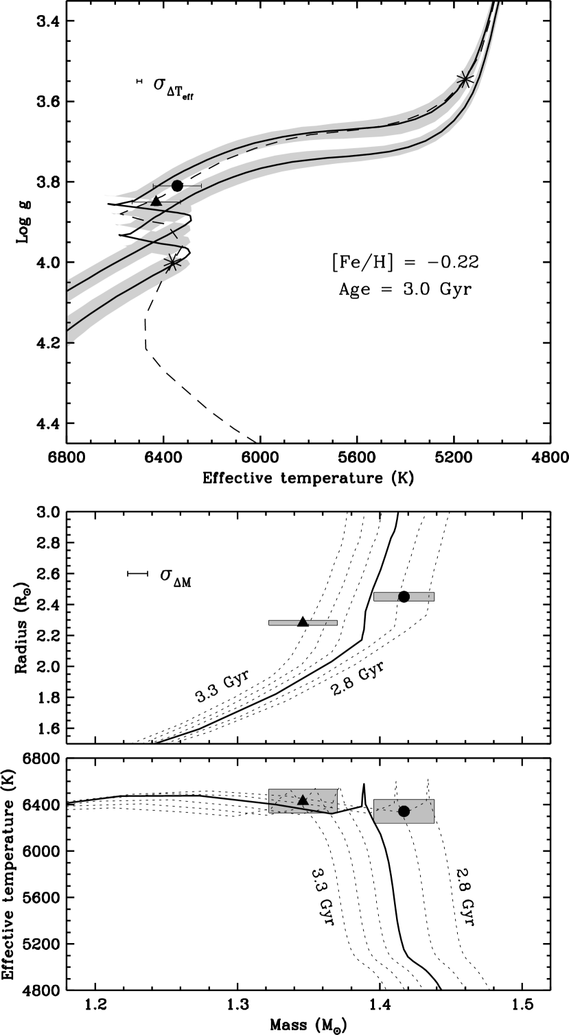
Figure 5.— Measurements for AQ Ser compared against the Yonsei-Yale stellar evolution models (Yi et al., 2001; Demarque et al., 2004) for $Z=0.0113$, corresponding to ${\rm[Fe/H]}=-0.22$ for these calculations ($Z_{\sun}=0.0181$; Grevesse & Noels, 1993a). Interpolations in mass, metallicity, and age were performed with routines provided by the modelers. The $\alpha$-element enhancement is assumed to be [$\alpha$/Fe] = 0.0. Top: Evolutionary tracks for the measured masses are shown with solid lines, the shaded area indicating the uncertainty in the location of the tracks stemming from the mass errors. The filled circle and triangle correspond to the more massive and less massive star, respectively. The best-fit isochrone for an age of 3.0 Gyr is shown with a dashed line. The predicted mass ratio for two evolved stars of this age so near each other in this part of the diagram is $q=1.0028$, which is significantly closer to unity than measured. This is illustrated with the asterisks, which mark the stars’ location on the isochrone for their measured masses. Bottom: Mass/radius and mass/temperature diagrams showing isochrones in steps of 0.1 Gyr from 2.8 to 3.3 Gyr. The solid line represents the best-fit isochrone from the top panel, and we indicate also the uncertainty in the mass difference.

An equivalent way of interpreting the discrepancy is in terms of age, as noted earlier. The lower panels of Figure 5 show the predictions from the Yonsei-Yale models for the radius and temperature as a function of mass, along with isochrones for a range of ages. The more massive star is better fit at a younger age than the secondary, the difference being about 0.45 Gyr (or 15%), as seen more clearly in the mass/radius plane. Isochrones in this diagram are mostly vertical for stars of this size, so the significance of the age difference depends largely on the mass separation. The mass uncertainties shown by the shaded boxes represent total errors; the error in the mass difference, $\sigma_{\Delta M}$, is considerably smaller and is also indicated in the figure. Therefore, the age discrepancy is highly significant.

As mentioned in Sect. 5, AQ Ser lacks a spectroscopic determination of [Fe/H] and only a photometric estimate is available. While the model comparisons above suggest a metallicity fairly close to that estimate, the solutions are not unique. We find that it is possible to obtain similarly good fits for somewhat lower values of [Fe/H], with the stars being at the end of the main-sequence phase rather than past the “blue hook”. We illustrate this with a third set of models from the Victoria-Regina series (VandenBerg et al., 2006). These calculations use a different description of overshooting based on a parametrized version of the Roxburgh criterion (Roxburgh, 1978; Baker & Kuhfuß, 1987; Roxburgh, 1989), in which the effect is assumed to ramp up between masses of 1.15 and 1.70 $M_{\sun}$ for compositions near solar. Figure 6 (top) shows a best-fit isochrone in the $\log g$ vs. $T_{\rm eff}$ diagram that places the stars in the Hertzprung gap, but as before it requires a mass ratio very near unity ($q=1.0008$) at odds with the measured value at the 4.8$\sigma$ level. This best fit corresponds to an age of 2.9 Gyr and ${\rm[Fe/H]}=-0.20$. In the bottom panel an equally good fit is achieved for an age of 2.3 Gyr and ${\rm[Fe/H]}=-0.30$ that accommodates the stars on the main sequence with the degree of overshooting prescribed in the models. However, even here theory would require the masses to be nearly the same ($q=1.0169$) to satisfy the age constraint, which is still in disagreement with the spectroscopic value at the 3.4$\sigma$ level. Perhaps as importantly, the measured radii or temperatures are not reproduced at the measured masses (see Figure 6). The ages required to match them are again younger for the more massive component, by about the same amount as in the post-main-sequence solution.

Figure 6.— Similar to the top panel of Figure 5, showing the comparison of the measurements for AQ Ser against the Victoria-Regina models (VandenBerg et al., 2006). Age interpolation was performed with the routines provided by the modelers. Top: Isochrones are shown for ages of 2.7 to 3.1 Gyr, with the best-fit model represented with the solid line for an age of 2.9 Gyr. This fit has $Z=0.0125$ (or ${\rm[Fe/H]}=-0.20$ with $Z_{\sun}=0.0188$; Grevesse & Noels, 1993b), and places the stars beyond the point of hydrogen exhaustion. The predicted mass ratio matching the measured radii and temperatures is $q=1.0008$, much smaller than observed. Bottom: Alternate solution in which the best-fit metallicity and age ($Z=0.0100$ or ${\rm[Fe/H]}=-0.30$, and 2.3 Gyr) were adjusted in such a way as to permit the stars to be in a more likely evolutionary state just prior to the blue hook. The mass ratio predicted by theory ($q=1.0169$) is still significantly smaller than measured. Isochrones are shown for ages of 2.1 to 2.5 Gyr. In both panels the asterisks mark the location of the stars on the best-fit isochrone according to their measured mass.

A similar exercise with the PARSEC models from the Padova group (Bressan et al., 2013), which employ yet another prescription for overshooting, again allows two qualitatively different solutions. The post-main-sequence scenario strongly disagrees with the measured mass ratio, and a lower metallicity scenario ($Z=0.0085$, or ${\rm[Fe/H]}=-0.25$ for $Z_{\sun}=0.01524$; Caffau et al., 2011) with the stars at the end of the main-sequence still requires a mass ratio of $q=1.0153$ that is lower than our spectroscopic result at the 3.5$\sigma$ level. Thus, all models seem to fail to match the observations for AQ Ser at a single age, pointing to a fundamental problem with theory likely related to overshooting.

7. Discussion

The most common way in which the degree of overshooting has been calibrated in stellar evolution models is by means of star clusters, and in particular through the comparison of isochrones to the blue-hook region in the color-magnitude diagram (CMD). The drawbacks are that this can be affected by contamination of the CMD by field stars, unresolved binary systems, or variable stars, by uncertainties in the chemical composition of the cluster, and even by systematics from the color/temperature transformations. Furthermore, the main property of stars — their absolute mass — is generally not known for any object along the CMD of the clusters most frequently used for this type of comparison. An alternate way of calibrating $\alpha_{\rm ov}$ is by means of eclipsing binary systems, where masses and radii are precisely known (see, e.g., Ribas et al., 2000). With this method the latter authors found a relatively strong mass (and possibly metallicity) dependence of overshooting for stars in the 2–12 $M_{\sun}$ range, although subsequent studies reported the mass dependence to be less pronounced and more uncertain (Claret, 2007).

The special location of AQ Ser in the H-R diagram makes it a uniquely sensitive test of convective core overshooting in current models of stellar evolution. As shown above, the measured mass ratio is different enough from unity that stars with radii and temperatures as similar as they are in this system cannot possibly be in the post-main-sequence phase. This constitutes clear evidence that mixing beyond the core (overshooting) is required. While early support for the need of extra mixing was shown nearly 25 years ago by Andersen et al. (1990) from the inordinately large number of B- and A-type eclipsing systems that appeared to be in the Hertzprung gap, the present system represents a particularly compelling demonstration. However, AQ Ser shows an additional problem, which is that even with the inclusion of overshooting and the freedom to adjust the metallicity in the models so as to accommodate the stars at the very end of the main-sequence phase, current calculations are still unable to match the well measured radius and temperature difference at the measured masses. Theory requires the stars to have masses much more similar to each other ($q\approx 1.016$) than they are observed to be ($q=1.054\pm 0.011$), a difference that seems beyond reasonable observational uncertainties.

This problem manifests itself also as an age discrepancy when attempting to fit models to each component separately: the more massive star appears systematically younger. Our comparisons in the previous section indicate that this difficulty is common to all models (and the age difference does not change much compared to the alternate post-main-sequence fit): the age difference is about 0.5 Gyr for the Granada models, 0.45 Gyr for the Yonsei-Yale models, 0.30 Gyr for the Victoria-Regina models, and 0.40 Gyr for the Padova models, all corresponding to 10–15% of the mean evolutionary age of the binary. Experiments with the Granada models in which we varied not only $\alpha_{\rm ov}$ but also the mixing length parameter $\alpha_{\rm ML}$ independently for each star, for different trial values of $Z$, gave mean ages ranging from 3.1 to 3.5 Gyr, but did not improve the situation regarding the age difference. We consistently found the predicted age for the more massive star to be younger than the other component.

Figure 7.— Masses and radii for all eclipsing binaries with accurately known parameters (relative uncertainties in $M$ and $R$ less than 3%) from Torres et al. (2010a), supplemented with measurements for CO And (Lacy et al., 2010), BF Dra (Lacy et al., 2012), and AQ Ser from the present work. The primary and secondary stars in each system are connected with a line. The shaded area corresponds to the blue hook region for solar metallicity, according to the Yonsei-Yale models. The dashed line represents the upper envelope of this region for a different metallicity of ${\rm Fe/H]}=-0.20$ near that of AQ Ser, and the dotted line at the bottom corresponds to the zero-age main sequence (ZAMS).

Similar age discrepancies in the same direction as we see were pointed out by Clausen et al. (2010) for several other well-measured F-type eclipsing systems with unequal masses in the range from 1.15 to 1.70 $M_{\sun}$. This is roughly the interval in which the models ramp up the strength of the overshooting, and is also approximately the mass range in which stars transition from having their energy production dominated by the p-p chain to the CNO cycle. The four systems studied by Clausen et al. (2010) for which age differences were noted are GX Gem, BW Aqr, V442 Cyg, and BK Peg. Of these, the first is the most similar to AQ Ser in terms of its evolutionary state. It is located just prior to the blue hook in the H-R diagram according to the models, although the component masses are more similar to each other than those in the AQ Ser system, so the age difference is less significant. Two other systems studied by us more recently are also quite near the end of the main sequence: CO And (Lacy et al., 2010) and BF Dra (Lacy et al., 2012). Although age anomalies were not mentioned in the original investigations of these binaries, a closer examination shows that both systems display age discrepancies similar to those seen previously, with the more massive component appearing younger. For CO And the age difference is about 0.3 Gyr (8%), and for BF Dra it is only $\sim$0.1 Gyr (4%), but still in the same direction. It is clear from these observations that a serious deficiency has been uncovered in current stellar evolution models for this mass range, which has not previously received much attention beyond the work of Clausen et al. (2010).

Figure 7 shows the location in the mass/radius diagram of all well-measured eclipsing binary systems studied by Clausen et al. (2010), as well as others from Torres et al. (2010a) having both components in the 1.15–1.70 $M_{\sun}$ range. To these we added CO And, BF Dra, and AQ Ser. The shaded area represents the region of the blue hook for solar composition, according to the Yonsei-Yale models, and an increase in the overshooting parameter would shift this region upward. AQ Ser is seen to be the most evolved system in this mass range, which perhaps explains the larger age discrepancy noted earlier.

Given that overshooting has a direct impact on evolution timescales, particularly for main-sequence stars in the more advanced stages, it is natural to suspect that the simplified treatment of this phenomenon in current models has something to do with their difficulty in matching the measured properties of binaries at a single age. However, from our tests with AQ Ser the explanation does not appear to be a simple difference in $\alpha_{\rm ov}$ for the two components, and may be more complex, involving, e.g., a dependence of overshooting on the state of evolution, in addition to mass and metallicity. To our knowledge the discrepancies highlighted by AQ Ser and the other systems mentioned above have not been investigated in detail for more massive stars. Although such a study is beyond the scope of the present work, it could well provide important clues about the nature of what we consider one of the outstanding problems of stellar evolution theory.

References

- Alencar & Vaz (1997) Alencar, S. H. P., & Vaz, L. P. R. 1997, A&A, 326, 257
- Alencar et al. (1999) Alencar, S. H. P., Vaz, L. P. R., & Nordlund, Å. 1999, A&A, 346, 556
- Allard & Hauschildt (1995) Allard, F., & Hauschildt, P. H. 1995, ApJ, 445, 433
- Allard et al. (1997) Allard, F., Hauschildt, P. H., Alexander, D. R., & Starrfield, S. 1997, ARA&A, 35, 137
- Andersen et al. (1990) Andersen, J., Clausen, J. V., & Nordström, B., 1990, ApJ, 363, L33
- Baker & Kuhfuß (1987) Baker, N. H., & Kuhfuß, R. 1987, A&A, 185, 117
- Bressan et al. (2013) Bressan, A., Marigo, P., Girardi, L., Salasnich, B., Dal Cero, C., Rubele, S., & Nanni, A. 2013, MNRAS, in press (arXiv:1208.4498)
- Caffau et al. (2011) Caffau, E., Ludwig, H.-G., Steffen, M., Freytag, B., & Bonifacio, P. 2011, Sol. Phys., 268, 255
- Cardelli et al. (1989) Cardelli, J. A., Clayton, G. C., & Mathis, J. S. 1989, ApJ, 345, 245
- Casagrande et al. (2010) Casagrande, L., Ramírez, I., Meléndez, J., Bessell, M., & Asplund, M. 2010, A&A, 512, 54
- Chiosi et al. (1992) Chiosi, C., Bertelli, G., & Bressan, A. 1992, ARA&A, 30, 235
- Chiosi (1999) Chiosi, C. 1999, in ASP Conf. Ser. 173, Theory and Tests of Convection in Stellar Structure, eds. A. Giménez, E. P. Guinan & B. Montesinos (San Francisco: ASP), 9
- Claret (2000) Claret, A. 2000, A&A, 363, 1081
- Claret (2004) Claret, A. 2004, A&A, 424, 919
- Claret (2007) Claret, A. 2007, A&A, 475, 1019
- Clausen et al. (2010) Clausen, J. V., Frandsen, S., Bruntt, H., Olsen, E. H., Helt, B. E., Gregersen, K., Juncher, D., & Krogstrup, P. 2010, A&A, 516, A42
- Crawford (1975) Crawford, D. L. 1975, AJ, 80, 955
- Cutri et al. (2003) Cutri, R. M. et al. 2003, The 2MASS All-Sky Catalog of Point Sources, Univ. of Massachusetts and Infrared Processing and Analysis Center (IPAC/California Institute of Technology)
- Demarque et al. (2004) Demarque, P., Woo, J.-H., Kin, Y.-C., & Yi, S. K. 2004, ApJS, 155, 667
- Drimmel et al. (2003) Drimmel, R., Cabrera-Lavers, A., & López-Corredoira, M. 2003, A&A, 409, 205
- Droege et al. (2006) Droege, T. F., Richmond, M. W., & Sallman, M. 2006, PASP, 118, 1666
- Flower (1996) Flower, P. J. 1996, ApJ, 469, 355
- Grauer et al. (2008) Grauer, A. D., Neely, A. W., & Lacy, C. H. S. 2008, PASP, 120, 992
- Grevesse & Sauval (1998) Grevesse, N., & Sauval, A. J. 1998, Space Sci. Rev., 85, 161
- Grevesse & Noels (1993a) Grevesse, N., & Noels, A. 1993a, in Origin and Evolution of the elements, ed. N. Prantzos, E. Vangioni-Flam, & M. Cassé (Cambridge: Cambridge Univ. Press), 14
- Grevesse & Noels (1993b) Grevesse, N., & Noels, A. 1993b, Phys. Scr., T47, 133
- Hakkila et al. (1997) Hakkila, J., Myers, J. M., Stidham, B. J., & Hardmann, D. H. 1997, AJ, 114, 2043
- Henden et al. (2012) Henden, A. A., Levine, S. E., Terrell, D., Smith, T. C., & Welch, D. 2012, J. American Association of Variable Star Observers, 40, 430
- Høg et al. (2000) Høg, E., Fabricius, C., Makarov, V. V., Urban, S., Corbin, T., Wycoff, G., Bastian, U., Schwekendiek, P., & Wicenec, A. 2000, A&A, 355, L27
- Hauschildt et al. (1997a) Hauschildt, P. H., Baron, E., & Allard, F. 1997a, ApJ, 483, 390
- Hauschildt et al. (1997b) Hauschildt, P. H., Allard, F., Alexander, D.R., & Baron, E. 1997b, ApJ, 488, 428
- Hilditch & Hill (1975) Hilditch, R. W., & Hill, G. 1975, MmRAS, 79, 101
- Hill et al. (1975) Hill, G., Hilditch, R. W., Younger, F., & Ficher, W. A. 1975, MmRAS, 79, 131
- Hoffmeister (1935) Hoffmeister, C. 1935, Astron. Nachr., 255, 401
- Høg et al. (2000) Høg, E., Fabricus, C., Makarov, V.V., Urban, S., Corbin, T., Wycoff, G., Bastian, U., Schwekendick, P., & Wicenec, A. 2000, A&A, 355, 27
- Kwee & van Woerden (1956) Kwee, K.K. & van Woerden, H. 1956, BAN, 12, 327
- Lacy et al. (2010) Lacy, C. H. S., Torres, G., Claret, A., Charbonneau, D., & O’Donovan, F. T. 2010, AJ, 139, 2347
- Lacy et al. (2012) Lacy, C. H. S., Torres, G., Fekel, F. C., Sabby, J. A., & Claret, A. 2012, AJ, 143, 129
- Latham (1992) Latham, D. W. 1992, in IAU Coll. 135, Complementary Approaches to Double and Multiple Star Research, ASP Conf. Ser. 32, eds. H. A. McAlister & W. I. Hartkopf (San Francisco: ASP), 110
- Latham et al. (2002) Latham, D. W., Stefanik, R. P., Torres, G., Davis, R. J., Mazeh, T., Carney, B. W., Laird, J. B., & Morse, J. A. 2002, AJ, 124, 1144
- Latham et al. (1996) Latham, D. W., Nordström, B., Andersen, J., Torres, G., Stefanik, R. P., Thaller, M., & Bester, M. 1996, A&A, 314, 864
- Nordström et al. (1994) Nordström, B., Latham, D. W., Morse, J. A., Milone, A. A. E., Kurucz, R. L., Andersen, J., & Stefanik, R. P. 1994, A&A, 287, 338
- Pinsonneault et al. (1991) Pinsonneault, M. H., Deliyannis, C. P., & Demarque, P. 1991, ApJ, 367, 239
- Popper (1980) Popper, D. M. 1980, ARA&A, 18, 115
- Press et al. (1992) Press, W. H., Teukolsky, S. A., Vetterling, W. T., & Flannery, B. P. 1992, Numerical Recipes, (2nd. Ed.; Cambridge: Cambridge Univ. Press), 650
- Ribas et al. (2000) Ribas, I., Jordi, C., & Giménez, Á. 2000,, MNRAS, 318, L55
- Roxburgh (1978) Roxburgh, I. W. 1978, A&A, 65, 281
- Roxburgh (1989) Roxburgh, I. W. 1989, A&A, 211, 361
- Sandberg Lacy et al. (2008) Sandberg Lacy, C. H., Torres, G., & Claret, A. 2008, AJ, 135, 1757
- Schlegel et al. (1998) Schlegel, D. J., Finkbeiner, D. P., & Davis, M. 1998, ApJ, 500, 525
- Schmidt-Kaler (1982) Schmidt-Kaler, Th. 1982, in Landolt-Börnstein, Numerical Data and Functional Relationships in Science and Technology, Vol. 2, eds. K. Schaifers & H. H. Voigt (Berlin: Springer)
- Schwarzschild (1906) Schwarzschild, K. 1906, Göttingen Nachr., 13, 41
- Soloviev (1951) Soloviev, A . V. 1951, Perem. Zvezdy, 7, No. 6, 325
- Torres et al. (2010a) Torres, G., Andersen, J., Giménez, A. 2010a, A&A Rev., 18, 67
- Torres (2010b) Torres, G. 2010b, AJ, 140, 1158
- Torres et al. (1997) Torres, G., Stefanik, R. P., Andersen, J., Nordström, B., Latham, D. W., & Clausen, J. V. 1997, AJ, 114, 2764
- Torres et al. (2002) Torres, G., Neuhäuser, R., & Guenther, E. W. 2002, AJ, 123, 1701
- VandenBerg et al. (2006) VandenBerg, D. A., Bergbusch, P. A., & Dowler, P. D. 2006, ApJS, 162, 375
- Vaz et al. (2007) Vaz, L. P. R., Andersen, J., & Claret, A. 2007, A&A, 469, 285
- Wilson (1979) Wilson, R. E. 1979, ApJ, 234, 1054
- Wilson (1993) Wilson, R. E. 1993, in New Frontiers in Binary Star Research, eds. K.C. Leung and L.-S. Nha, APS Conf. Series, 38, 91
- Wilson & Devinney (1971) Wilson, R. E., & Devinney, E. J. 1971, ApJ, 166, 605
- Yi et al. (2001) Yi, S., Demarque, P., Kin, Y.-C., Lee, Y.-W., Ree, C. H., Lejeune, T., & Barnes, S. 2001, ApJS, 136, 417
- Zucker & Mazeh (1994) Zucker, S., & Mazeh, T. 1994, ApJ, 420, 806