Non-Gaussianity of the Cosmic Infrared Background anisotropies I : Diagrammatic formalism and application to the angular bispectrum

Abstract

We present the first halo model based description of the Cosmic Infrared Background (CIB) non-Gaussianity (NG) that is fully parametric. To this end, we introduce, for the first time, a diagrammatic method to compute high order polyspectra of the 3D galaxy density field. It allows an easy derivation and visualisation of the different terms of the polyspectrum. We apply this framework to the power spectrum and bispectrum, and we show how to project them on the celestial sphere in the purpose of the application to the CIB angular anisotropies. Furthermore, we show how to take into account the particular case of the shot noise terms in that framework. Eventually, we compute the CIB angular bispectrum at 857 GHz and study its scale and configuration dependencies, as well as its variations with the halo occupation distribution parameters. Compared to a previously proposed empirical prescription, such physically motivated model is required to describe fully the CIB anisotropies bispectrum. Finally, we compare the CIB bispectrum with the bispectra of other signals potentially present at microwave frequencies, which hints that detection of CIB NG should be possible above 220 GHz.

1 Introduction

The structuration of the large scale structures and galaxies in the Universe is a long-standing field of research in cosmology, theoretically as well as observationally. Of particular interest is the clustering of galaxies as the latter are biased tracers of the underlying dark matter field. Although perturbation theory (see Bernardeau et al., 2002, for a review) may describe the clustering of dark matter up to mildly non-linear scales and epochs, it breaks down in the regime of highly non-linear gravitational infall and does not prescribe the behaviour of galaxies and baryonic physics with respect to dark matter. Neyman & Scott (1952) pioneered the description of galaxies as distributed in clusters, which were later identified as dark matter halos as the dark matter paradigm became popular. This latter description has become a fruitful tool, assuming that galaxy properties are determined by the physical characteristics of the host halo, as dark matter simulations have become available. Indeed these simulations have permitted to prescribe the distribution of mass inside halos (a.k.a. the density profile), their abundance and spatial distribution (e.g. Navarro et al., 1997). Then analytic or semi-analytic models prescribing the distribution and properties of different galaxy populations may be built (e.g. De Lucia & Blaizot, 2007). A common analytical tool is the halo model. In this framework, all dark matter is assumed to be bound up in halos which are populated with galaxies thanks to the halo occupation distribution (HOD). The standard HOD rules the mean number of galaxies in a halo depending on its mass (Berlind et al., 2003; Kravtsov et al., 2004). Such models have been widely used to reproduce the 2-point correlation function of optically-selected galaxies, see e.g. Tinker et al. (2010); Coupon et al. (2012) and references therein for the most recent analyses. Most applications to date have concentrated on 2-point statistics, i.e. real-space 2-point correlation function or –auto and cross– power spectrum of tracers.
One tracer of galaxies and dark matter that has been studied thanks to the halo model is the Cosmic Infrared Background (CIB). It was first discovered by Puget et al. (1996), and it stems from the cumulative emission of dusty star-forming galaxies (DSFG). The UV emission from young stars heats up the surrounding dust which consequently reemits in the infrared (from 8 $\mu$m  to 1 mm) with a typical greybody law. The CIB is consequently a tracer of star formation, with lower frequencies ($\nu<220$ GHz) tracing star formation at high redshifts (see e.g. Pénin et al., 2012), as their emission is redshifted into the Far-IR/sub-millimeter domain. Resolutions of current instruments permit to resolve directly only a small fraction of the CIB into individual sources, in particular at far-IR frequencies ($<$857 GHz) where most of the CIB is unresolved so that sources produce brightness fluctuations generating the CIB anisotropies. The CIB fluctuations trace the clustering of the underlying DSFG and their angular power spectra have been measured, in the last few years, over a wide range of wavelengths and scales (Lagache et al., 2007; Viero et al., 2009; Planck Collaboration et al., 2011a; Amblard et al., 2011; Thacker et al., 2012; Pénin et al., 2012; Planck Collaboration et al., 2013). These measurements are usually modeled in the context of the halo model associated to a model of evolution of galaxies (Cooray et al., 2010; Pénin et al., 2012). Until recently, only the power spectrum of the CIB anisotropies had been measured, however statistical information is contained in the higher order moments.

The hierarchy of n-point correlation functions, for n up to infinity, characterises statistically a field, univoquely under some regularity conditions. In particular beyond n=2 it probes the non-Gaussianity of the field. Non-Gaussianity (NG) studies have emerged as a research field of interest, as they bring information complementary to power spectrum (or 2-point correlation function) analyses. They are of particular interest for the Cosmic Microwave Background (CMB), for instance, the study of primordial NG discriminates inflation models which are degenerate at the power spectrum level. Lately, the Planck NG constraints have ruled out several primordial models, in particular the possibility of ekpyrotic/cyclic Universe (Planck Collaboration XXIV, 2013).

Nevertheless, such measurements are delicate as millimeter observations dedicated to the CMB are contaminated by foregrounds which are non-Gaussian. Extragalactic point-sources are of particular importance because they are present all over the sky and the fainter ones cannot be detected nor masked. At CMB frequencies, two types of extragalactic point-sources are present : radio-loud sources powered by an Active Galactic Nucleus (Toffolatti et al., 1999) and DSFG constituting the Cosmic Infrared Background (Lagache et al., 2005). NG of these point-sources has first been looked for at radio frequencies with WMAP, focusing on radio sources which can be considered unclustered (Toffolatti et al., 1998). Bispectrum predictions based on number counts and measurement on WMAP data have been found in agreement (Komatsu et al., 2003) and have permitted to quantify the level of unresolved sources in WMAP maps. At higher frequencies, non-Gaussianity of DSFG has been pioneered by Argüeso et al. (2003); González-Nuevo et al. (2005), and lately Lacasa et al. (2012) with a phenomenological prescription based on the clustered power spectrum. Prior to the present study, no physically-based model of the CIB NG was proposed.

This article builds a halo model description of galaxy clustering at high orders that we apply to predict the NG of CIB anisotropies. This allows for a full model for the CIB anisotropies which, given a galaxy emission model and HOD parameters, computes the power spectrum as well as the bispectrum, and possibly higher order moments. The clustering part of the model is fully parametric which will, at longer term, allow us to constrain these parameters using as much statistical information from the data as possible. In a companion article (Pénin et al., 2013), referred to as Paper2 hereafter, we carry out a Fisher analysis forecast of how the degeneracies of these parameters are broken when combining power spectra and bispectra constraints. In addition, we study in details, amongst others, the variation of the CIB angular bispectrum with respect to the models of evolution of galaxies, and the frequency evolution of the redshift-halo mass contributions to the bispectrum.

The present article is organised as follows. Section 2 details the halo model formalism, accounting for the shot-noise due to the discreteness of galaxies, the occupation statistics (HOD) and shows the resulting 3D power spectrum. In Sect.3, we derive the galaxy bispectrum and describe a diagrammatic method to carry the derivation to higher orders. Sect.4 introduces harmonic transform of correlation functions on the sky and shows how the 3D polyspectra of a signal project onto the sphere. Taking the example of the CIB, we discuss how the shot-noise terms must be accounted for and the necessary regularisation at low redshift. The resulting CIB angular bispectrum is shown with its different terms in Sect.5 as well as their dependencies on the HOD parameters. We also investigate the halo-mass contributions to the galaxy bispectrum. Eventually, in Sect.6, we compare the obtained CIB angular bispectrum to a previously proposed prescription and to the bispectra of other signals present at microwave frequencies, namely radio sources and CMB. We finally conclude in Sect.7.

2 Galaxy clustering with the halo model

The most common tool to measure the clustering of galaxies is the two-point correlation function. At first, such measurements were well reproduced by a simple power law (Davis & Peebles, 1983; Madgwick et al., 2003; Le Fèvre et al., 2005). Nevertheless, the progress in the field of large scale surveys enabled more accurate measurements that rule out such simple modeling (e.g. Zehavi et al., 2004) as they display a cut-off at intermediate scales. A more complex modeling was required leading to the wide use of the halo model (e.g. Cooray & Sheth, 2002). In that framework, dark matter is assumed to be bound up in halos which are virialised spherical objects $\Delta_{\mathrm{vir}}$ times denser than the background. The introduction of the galaxies within the halos is done through the Halo Occupation Distribution (Kravtsov et al., 2004; Tinker & Wetzel, 2010). This modeling has proven to be a very convenient analytical tool to reproduce and interpret the non-linear clustering of dark matter halos as well as that of galaxies (e.g. Coupon et al., 2012). This section summarizes the ingredient of the halo model necessary to predict the galaxy distribution, and we show how to treat self-consistently the discreteness of galaxies.

2.1 Halo framework

In the halo model framework, galaxies reside in dark matter halos that are assumed spherical. Hence the galaxy density field at a given point $\mathbf{x}$ reads (redshift dependencies are implicit throughout this article, we state them explicitly when needed) :

$$n_{\mathrm{gal}}(\mathbf{x})=\sum_{i}n_{\mathrm{gal}}(\mathbf{x}|i)$$ (1)

with $i$ being the halo index. In the literature, $n_{\mathrm{gal}}(\mathbf{x}|i)$ is assumed, implicitly or explicitly, to be a smooth distribution following the halo density profile. However, galaxies are discrete objects ; hence we write :

$$n_{\mathrm{gal}}(\mathbf{x}|i)=\sum_{j=1}^{N_{\mathrm{gal}}(i)}\theta(\mathbf{x}-\mathbf{x}_{j})$$ (2)

with $j$ being the index of the random galaxies, $N_{\mathrm{gal}}(i)$ being the –random– number of galaxies in the halo $i$, $x_{j}$ is the –random– position of the $j$th galaxy, and $\theta(x)$ is the galaxy profile. We assume here after that galaxies are drawn independently in the halo.
Equation 1 can then be rewritten as:

$$n_{\mathrm{gal}}(\mathbf{x}) = \int\mathrm{d}M\,\mathrm{d}^{3}\mathbf{x}_{\mathrm{h}}\sum_{i}\delta(M-M_{i})\,\delta^{(3)}(\mathbf{x}_{\mathrm{h}}-\mathbf{x}_{i})$$ (3)

$$\times\int\mathrm{d}^{3}\mathbf{x}_{\mathrm{g}}\sum_{j=1}^{N_{\mathrm{gal}}(i)}\delta^{(3)}(\mathbf{x}_{\mathrm{g}}-\mathbf{x}_{j})\,\theta(\mathbf{x}-\mathbf{x}_{j})$$

with $M_{i}$ and $\mathbf{x}_{i}$ the mass and position of the dark matter halo $i$. This equation serves as the basis for the computation of the galaxy clustering throughout this article.
Furthermore, we make the following set of assumptions for the galaxy distribution :

• halos are spherical. This is a common assumption in halo models ; inclusion of halo shapes was shown to have a 5-10% effect on the 3D bispectrum by Smith et al. (2006).

• the number of galaxies $N_{\mathrm{gal}}(i)$ ($=N_{\mathrm{gal}}(M_{i})$) is drawn from the HOD and depends on the mass $M_{i}$ of the halo (see Sect.2.2).

• the galaxy positions follow the dark matter halo profile. They are drawn from a distribution whose pdf is the normalised halo profile $u(\mathbf{x}|M)$ centered on the halo center :

  $$p(\mathbf{x}_{j}|i)=u(\mathbf{x}_{j}-\mathbf{x}_{i}|M_{i})$$ (4)

• the galaxy profile $\theta(x)$ is a Dirac $\delta^{(3)}(x)$. This assumption holds since the scales probed are larger than the galaxy size.

The galaxy density field may then be characterised with a hierarchy of n-point correlation functions of $n_{\mathrm{gal}}$. At first order (n=1), the mean number of galaxies per comoving volume, is :

$$\overline{n}_{\mathrm{gal}}=\int\mathrm{d}M\,\langle N_{\mathrm{gal}}(M)\rangle\,\frac{\mathrm{d}n_{\mathrm{h}}}{\mathrm{d}M}$$ (5)

where $\frac{\mathrm{d}n_{\mathrm{h}}}{\mathrm{d}M}$ is the number of halos with mass $M$ per comoving volume, i.e., the halo mass function. It is convenient to define the galaxy density contrast as :

$$\delta_{\mathrm{gal}}(\mathbf{x})=\frac{n_{\mathrm{gal}}(\mathbf{x})-\overline{n}_{\mathrm{gal}}}{\overline{n}_{\mathrm{gal}}}$$ (6)

In the following, we will derive the correlation functions of $\delta_{\mathrm{gal}}$ and their Fourier transform. To this end we need to explicit the behaviour of the number of galaxies occupying a halo.

2.2 Occupation statistics

High resolution dissipationless simulations as well as semi-analytic and $N$-body+gas dynamics studies show that the number of galaxies within a single halo depends on halo mass with a shape consisting of a step, a shoulder and a power-law tail at high mass (e.g. Berlind et al., 2003; Kravtsov et al., 2004). This behaviour can be understood when the number of galaxies, described as a random distribution, is split into the contribution from central galaxies and that of satellite ones $N_{\mathrm{gal}}=N_{\mathrm{cen}}+N_{\mathrm{sat}}$. The former is described as a step-like function while the latter is a power law. High resolution simulations have brought a lot of progress in the modeling of these two contributions (e.g. Tinker & Wetzel, 2010).

The HOD provides us with the number of galaxies in a halo ; $N_{\mathrm{cen}}$ takes either the value of 0 or 1, and the presence of satellite galaxies is conditioned to $\{N_{\mathrm{cen}}=1\}$. If $N_{\mathrm{cen}}=1$, the number of satellites is drawn from a Poisson distribution (see Zheng et al., 2005) with mean $\overline{n}_{\mathrm{sat}}$ (in the following, over-bar denotes the average conditioned to $\{N_{\mathrm{cen}}=1\}$). Hence we have :

$$\langle N_{\mathrm{sat}}\rangle=P(N_{\mathrm{cen}}\!=\!1)\times\overline{n}_{\mathrm{sat}}=\langle N_{\mathrm{cen}}\rangle\times\overline{n}_{\mathrm{sat}}$$ (7)

Using the properties of the Poisson distribution, we can then compute the expectation values that will be used in the following sections:

$$\langle N_{\mathrm{gal}}\rangle = P(N_{\mathrm{cen}}\!=\!1)\times(1+\overline{n}_{\mathrm{sat}})$$ (8)

$$= \langle N_{\mathrm{cen}}\rangle+\langle N_{\mathrm{sat}}\rangle$$

$$\langle N_{\mathrm{gal}}(N_{\mathrm{gal}}-1)\rangle = P(N_{\mathrm{cen}}\!=\!1)\times\overline{(n_{\mathrm{sat}}+1)n_{\mathrm{sat}}}$$ (9)

$$= \langle N_{\mathrm{cen}}\rangle(\overline{n}_{\mathrm{sat}}^{2}+2\,\overline{n}_{\mathrm{sat}})$$

$$\langle N_{\mathrm{gal}}\,(N_{\mathrm{gal}}-1)(N_{\mathrm{gal}}-2)\rangle = P(N_{\mathrm{cen}}\!=\!1)$$ (10)

$$\times\overline{(n_{\mathrm{sat}}+1)\,n_{\mathrm{sat}}\,(n_{\mathrm{sat}}-1)}$$

$$= \langle N_{\mathrm{cen}}\rangle\left(\overline{n}_{\mathrm{sat}}^{3}+3\overline{n}_{\mathrm{sat}}^{2}\right)$$

We take the mean number of central galaxies as in Pénin et al. (2012):

$$\langle N_{\mathrm{cen}}\rangle=P(N_{\mathrm{cen}}\!=\!1)=\frac{1}{2}\left[1+\mathrm{erf}\left(\frac{\log M-\log M_{\mathrm{min}}}{\sigma_{\log M}}\right)\right]$$ (11)

and the mean number of satellites as:

$$\langle N_{\mathrm{sat}}\rangle=\frac{1}{2}\left[1+\mathrm{erf}\left(\frac{\log M-\log 2M_{\mathrm{min}}}{\sigma_{\log M}}\right)\right]\left(\frac{M}{M_{\mathrm{sat}}}\right)^{\alpha_{\mathrm{sat}}}$$ (12)

where, as for the rest of this article, we use base-10 logarithm.

Such expressions are motivated by hydrodynamical cosmological simulations (Berlind et al., 2003) as well as high-resolution collisionless simulations (Kravtsov et al., 2004). In this formulation, the HOD is thus characterised by four parameters : $M_{\mathrm{min}}$, the mass threshold above which a halo contains a central galaxy ; $\sigma_{\log M}$ describing the width of the transition from 0 to 1 central galaxy ; $M_{\mathrm{sat}}$ the typical mass above which a halo contains satellite galaxies ; and $\alpha_{\mathrm{sat}}$ the index of the power law for the number of satellites at large halo masses. Furthermore, $N_{\mathrm{sat}}$ has a cut-off of the same form as the central occupation but with a transition mass twice larger than that of the central galaxy. This prevents halos which have a low probability of hosting a central galaxy to contain satellite galaxies. Throughout this article we use $\log M_{\mathrm{min}}/M_{\odot}=12.6$, $\sigma_{\log M}=0.65$, $\log M_{\mathrm{sat}}/M_{\odot}=13.6$ and $\alpha_{\mathrm{sat}}=1.1$, unless otherwise stated (see Pénin et al., 2013).

2.3 Power spectrum

In the last decade, it has been shown that the 2-point correlation function of galaxies departs from a simple power law (Zehavi et al., 2004). In the framework of the halo model, this has been reproduced by splitting the total 2-point correlation function, or the angular power spectrum, into two contributions, the 1- and 2-halo terms. The discreteness of galaxies further adds a shot-noise term, which can be accounted for following a counts-in-cells approach (Peebles, 1980). We thus have :

$$P_{\mathrm{gal}}(k)=P^{\mathrm{1h}}_{\mathrm{gal}}(k)+P^{\mathrm{2h}}_{\mathrm{gal}}(k)+P^{\mathrm{shot}}_{\mathrm{gal}}(k)$$ (13)

The shot-noise contribution is given by

$$P^{\mathrm{shot}}_{\mathrm{gal}}(k)=\frac{1}{\overline{n}_{\mathrm{gal}}},$$ (14)

and will be examined in more detail in Sect.4.3. The 1- and 2-halo terms describe respectively the contribution of two galaxies within one same halo and that of two galaxies in two different halos. The 1-halo contribution is:

$$P^{\mathrm{1h}}_{\mathrm{gal}}(k)=\int\!\mathrm{d}M\,\frac{\mathrm{d}n_{\mathrm{h}}}{\mathrm{d}M}\frac{\langle N_{\mathrm{gal}}(M)(N_{\mathrm{gal}}(M)-1)\rangle}{\overline{n}_{\mathrm{gal}}^{2}}u(k|M)^{2}$$ (15)

where $u(k|M)$ is the Fourier transform of the normalised halo profile. Throughout this article, we use the Navarro-Frenk-White halo profile (Navarro et al., 1997), and the Sheth & Tormen mass function (Sheth & Tormen, 1999) that provides us with associated bias functions, in particular the second order bias $b_{2}(M)$, introduced in Sect.3.1, which will be needed for the bispectrum computation later on.
The 2-halo contribution writes:

$$P^{\mathrm{2h}}_{\mathrm{gal}}(k)=P_{\mathrm{lin}}(k)\left(\int\mathrm{d}M\,\frac{\langle N_{\mathrm{gal}}(M)\rangle\,\frac{\mathrm{d}n_{\mathrm{h}}}{\mathrm{d}M}}{\overline{n}_{\mathrm{gal}}}\,b_{1}(M)\,u(k|M)\right)^{2}$$

where $P_{\mathrm{lin}}(k)$ is the dark matter power spectrum predicted by linear theory (working at tree-level).

On scales larger than the typical halo size, $u(k|M)\rightarrow 1$ when $k\rightarrow 0$. Hence, the 1-halo term tends towards a constant while the 2-halo term tends towards the linear power spectrum. On small scales, the halo profile smoothes out both terms. For instance, the contribution of massive halos is smoothed at a smaller cut-off wavenumber compared to that of lower mass halos. The 1- and 2-halo terms of the power spectrum are exhibited in Fig. 1 at redshifts $z=0.1$ (left panel) and $z=1$ (right panel). Note that the $k$ range is different from a panel to another. Indeed, we compute the power spectrum at the wave-vectors which will project on observable angular scales on the sky (see Sect.5). As expected, we find that the 1-halo term dominates at small scales while the 2-halo term is more important at large scales. We also note that the 1-halo term increases clearly with time, by a factor $\sim$2, while the 2-halo does not significantly vary.

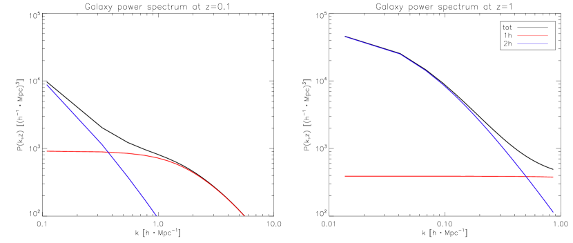
Figure 1: For the Navarro-Frenk-White halo profile and the Sheth & Tormen mass function we plot the 1-halo and 2-halo terms of the galaxy power spectrum at respectively $z$=0.1 (left panel) and $z$=1 (right panel). Note that the $k$ range is not identical between the plots.

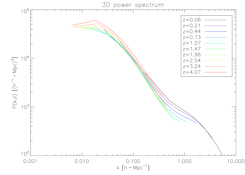
Figure 2: Total 3D galaxy power spectrum as a function of redshift

In Fig. 2, we show the evolution with redshift of the total galaxy power spectrum (1- and 2-halo terms). The spectrum decreases with increasing redshift up to $z$$\sim$2 beyond which it increases with redshift. This behaviour seems counter-intuitive as the linear dark-matter power spectrum, $P_{\mathrm{lin}}(k,z)$, decreases monotonically with increasing redshift. However, galaxies are biased tracers of matter and they are strongly biased at high redshift ($b_{\mathrm{gal}}\sim 5.5$ at $z$ $\sim$ 4) (Coupon et al., 2012; Jullo et al., 2012), which counterbalances the decrease of $P_{\mathrm{lin}}(k,z)$.

3 Higher orders with the halo model

As it is analytical, the halo model can be extended easily to higher orders. Indeed, it has been already used to compute the real-space 3-point correlation function (Wang et al., 2004), comparing favourably with simulations and measurements, as well as the bispectrum in redshift space (Smith et al., 2008), comparing again favourably with numerical simulations of dark matter.
In the following, we first summarize the 3D bispectrum computation and then we present a new diagrammatic method that can be used to compute the series of high order moments.

3.1 Bispectrum

The 3D galaxy bispectrum at a given redshift can be written as the sum of several terms (see detailed derivation in Appendix B, neglecting primordial non-Gaussianity as argued in the Appendix) :

$$B_{\mathrm{gal}}(k_{1},k_{2},k_{3},z) =B^{\mathrm{1h}}_{\mathrm{gal}}(k_{1},k_{2},k_{3},z)+B^{\mathrm{2h}}_{\mathrm{gal}}(k_{1},k_{2},k_{3},z)$$

$$+B^{\mathrm{3-halo}}_{\mathrm{gal}}(k_{1},k_{2},k_{3},z)+B^{\mathrm{shot2g}}_{\mathrm{gal}}(k_{1},k_{2},k_{3},z)$$

$$+B^{\mathrm{shot1g}}_{\mathrm{gal}}(k_{1},k_{2},k_{3},z)$$ (16)

where the 1-halo term writes :

$$B^{\mathrm{1h}}_{\mathrm{gal}}(k_{1},k_{2},k_{3},z) =\int\mathrm{d}M\,\frac{\langle N_{\mathrm{gal}}(N_{\mathrm{gal}}-1)(N_{\mathrm{gal}}-2)\rangle}{\overline{n}_{\mathrm{gal}}^{3}(z)}\,\frac{\mathrm{d}n_{\mathrm{h}}}{\mathrm{d}M}$$

$$\qquad\times u(\mathbf{k}_{1}|M,z)\,u(\mathbf{k}_{2}|M,z)\,u(\mathbf{k}_{3}|M,z)$$ (17)

The 2-halo term writes :

$$B^{\mathrm{2h}}_{\mathrm{gal}}(k_{1},k_{2},k_{3},z) =\mathcal{G}_{1}(k_{1},k_{2},z)\;P_{\mathrm{lin}}(k_{3},z)\,\mathcal{F}_{1}(k_{3},z)$$

$$+\ \mathcal{G}_{1}(k_{1},k_{3},z)\;P_{\mathrm{lin}}(k_{2},z)\,\mathcal{F}_{1}(k_{2},z)$$

$$+\ \mathcal{G}_{1}(k_{2},k_{3},z)\;P_{\mathrm{lin}}(k_{1},z)\,\mathcal{F}_{1}(k_{1},z)\qquad$$ (18)

The 3-halo term writes :

$$B^{\mathrm{3-halo}}_{\mathrm{gal}}(k_{1},k_{2},k_{3},z) =\mathcal{F}_{1}(k_{1},z)\,\mathcal{F}_{1}(k_{2},z)\,\mathcal{F}_{1}(k_{3},z)$$

$$\times\left[F^{s}(\mathbf{k_{1}},\mathbf{k_{2}})\,P_{\mathrm{lin}}(k_{1},z)\,P_{\mathrm{lin}}(k_{2},z)+\mathrm{perm.}\right]$$

$$+\ \mathcal{F}_{1}(k_{1},z)\,\mathcal{F}_{1}(k_{2},z)\,\mathcal{F}_{2}(k_{3},z)$$

$$\quad\times P_{\mathrm{lin}}(k_{1},z)\,P_{\mathrm{lin}}(k_{2},z)+\mathrm{perm.}$$ (19)

with

$$\mathcal{F}_{1}(k,z)=\int\mathrm{d}M\frac{\langle N_{\mathrm{gal}}(M)\rangle}{\overline{n}_{\mathrm{gal}}(z)}\,\frac{\mathrm{d}n_{\mathrm{h}}}{\mathrm{d}M}(M,z)\,b_{1}(M,z)\,u(k|M,z).$$ (20)

where $b_{1}(M,z)$ is the first order bias,

$$\mathcal{F}_{2}(k,z)=\int\mathrm{d}M\frac{\langle N_{\mathrm{gal}}(M)\rangle}{\overline{n}_{\mathrm{gal}}(z)}\,\frac{\mathrm{d}n_{\mathrm{h}}}{\mathrm{d}M}(M,z)\,b_{2}(M,z)\,u(k|M,z)$$ (21)

where $b_{2}(M,z)$ is the second order bias,

$$\mathcal{G}_{1}(k_{1},k_{2},z)={} \int\mathrm{d}M\frac{\langle N_{\mathrm{gal}}(N_{\mathrm{gal}}-1)\rangle}{\overline{n}_{\mathrm{gal}}(z)^{2}}\,\frac{\mathrm{d}n_{\mathrm{h}}}{\mathrm{d}M}(M,z)\,b_{1}(M,z)$$

$$\qquad\times u(k_{1}|M,z)\,u(k_{2}|M,z)$$ (22)

and

$$F^{s}(\mathbf{k_{i}},\mathbf{k_{j}})=\frac{5}{7}+\frac{1}{2}\cos(\theta_{ij})(\frac{k_{i}}{k_{j}}+\frac{k_{j}}{k_{i}})+\frac{2}{7}\cos^{2}(\theta_{ij})$$ (23)

which stems from non-linear evolution at second order in perturbation theory (e.g., Fry, 1984; Gil-Marín et al., 2012).
In the following, we will note 3hcos the part of the 3-halo term containing the $F_{ij}$ kernel (i.e., the first term of Eq.19), and we note 3h the part involving the second order bias (i.e., the last lines of Eq.19) :

$$B^{\mathrm{3-halo}}_{\mathrm{gal}}(k_{123},z)=B^{\mathrm{3h}}_{\mathrm{gal}}(k_{123},z)+B^{\mathrm{3hcos}}_{\mathrm{gal}}(k_{123},z)$$ (24)

Eventually, the shot-noise terms are:

$$B^{\mathrm{shot1g}}_{\mathrm{gal}}(k_{1},k_{2},k_{3},z) =\frac{1}{\overline{n}_{\mathrm{gal}}^{2}(z)}$$ (25)

$$B^{\mathrm{shot2g}}_{\mathrm{gal}}(k_{1},k_{2},k_{3},z) =\frac{P^{\mathrm{clust}}_{\mathrm{gal}}(k_{1})+P^{\mathrm{clust}}_{\mathrm{gal}}(k_{2})+P^{\mathrm{clust}}_{\mathrm{gal}}(k_{3})}{\overline{n}_{\mathrm{gal}}(z)}$$ (26)

with $P^{\mathrm{clust}}_{\mathrm{gal}}(k)=P^{\mathrm{1h}}_{\mathrm{gal}}(k)+P^{\mathrm{2h}}_{\mathrm{gal}}(k)$. These terms will be examined in more details in Sect.4.3.

For illustration, Fig. 3 shows the 1-, 2- and 3-halo terms of the galaxy bispectrum at $z$=0.1 (left panel) and $z$=1 (right panel), in the equilateral configuration ($k_{1}=k_{2}=k_{3}$). Note that, due to projection effects, here again the $k$ range is not identical between the plots.

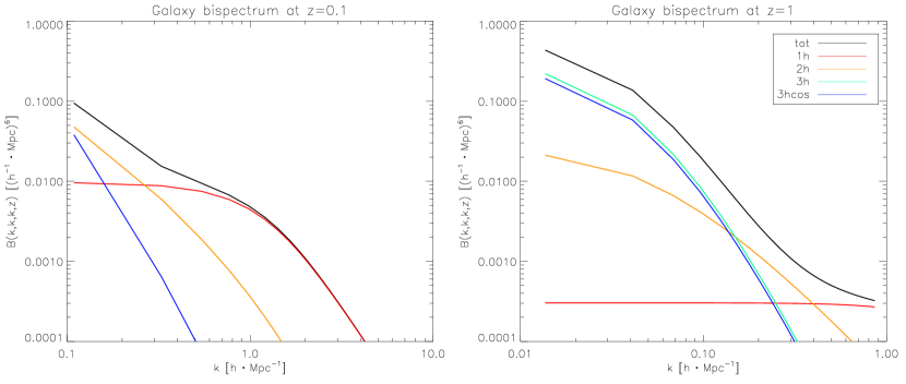
Figure 3: The 1-, 2- and 3-halo terms of the galaxy bispectrum at respectively $z$=0.1 (left panel) and $z$=1 (right panel). Note that the $k$ range is not identical between the plots.

We first note that the 2- and 3-halo terms dominate at large scales whereas the 1-halo term dominates at small scales. We see that all terms grow with time, the 1-halo having the fastest growth. We also note that the 3-halo term becomes negative at $z$=0.1. This comes from the fact that the second order bias can be either positive or negative depending on the halo mass and on the redshift. For halos with $M\sim 10^{13-14}M_{\odot}$ (which typically dominate the 3-halo term) $b_{2}$ is positive at high redshifts and it becomes negative at low redshifts (e.g., at $M=10^{13}M_{\odot}$ it changes sign at $z\sim 0.6$, while it changes sign at $z\sim 1.5$ at $M=10^{12}M_{\odot}$ and is always positive at $M=10^{14}M_{\odot}$).

Figure 4 shows the evolution of the total 3D bispectrum of the galaxies across redshifts. The bispectrum clearly increases with time, as gravitational infall produces non-linear structures so that the density field deviates more and more from its initially Gaussian distribution.

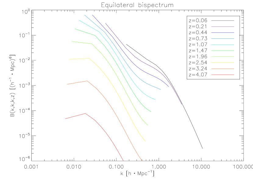
Figure 4: Total galaxy equilateral bispectrum as a function of redshift.

3.2 Diagrammatic and higher orders

The 3D galaxy density field may also be characterised with higher orders than the power spectrum and bispectrum. This is achieved through the use of polyspectra, where $\mathcal{P}^{(n)}_{\mathrm{gal}}(\mathbf{k}_{1\cdots n},z_{1\cdots n})$ is the polyspectrum of order $n$. See Appendix D for a comprehensive definition of polyspectra and their diagonal degrees of freedom.

We introduce here, for the first time, a diagrammatic method permitting the derivation of the equations of the 3D galaxy polyspectrum coming from the halo model. This approach is a generalisation of the formalism at second and third order, the power spectrum and bispectrum, respectively. It allows us to have a clear representation and understanding of the different terms involved. It further allows us to avoid cumbersome calculations at high order, by replacing them with diagram drawings.

The first step of the diagrammatic method that we propose here is to draw in the form of diagrams all the possibilities of putting $n$ galaxies in halo(s). Potentially, two or more galaxies can lie at the same point (“contracted”) for the shot-noise terms. Then for each diagram, the galaxies are labeled, e.g., from 1 to $n$, as well as the halos e.g. with $\alpha_{1}$ to $\alpha_{p}$. An illustration is given in Fig. 5 that displays the three diagrams for the power spectrum ; Fig.6 shows the six diagrams for the bispectrum ; and finally Fig.7 exhibits the 14 diagrams for the trispectrum.

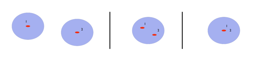
Figure 5: Diagrams for the 3D galaxy power spectrum. From left to right: (2-halo), (1-halo,2-galaxies), (1-halo,1-galaxy). Violet circles represent halos and red ellipses galaxies.

Each diagram produces a polyspectrum term. This term contains a prefactor $1/\overline{n}_{\mathrm{gal}}^{\,n}$ multiplied by an integral over the halo masses $\int\mathrm{d}M_{\alpha_{1}\cdots\alpha_{p}}$ of several factors. The following “Feynman”-like rules prescribe these different factors :

• for each halo $\alpha_{j}$ there is a corresponding :

  • halo mass function $\left.\frac{\mathrm{d}n_{\mathrm{h}}}{\mathrm{d}M}\right|_{M_{\alpha_{j}}}$

  • average of the number of galaxy uplets in that halo.
    e.g., $\langle N_{\mathrm{gal}}\rangle$ for a single galaxy in that halo, $\langle N(N-1)\rangle$ for a pair etc.

  • as many halo profiles $u(k|M_{\alpha_{j}})$ as different points, where $k=|\sum_{i\in\mathrm{point}}\mathbf{k}_{i}|$.
    For example $k=k_{i}$ for a non-contracted galaxy $i$, while $k=|\mathbf{k}_{i_{1}}+\cdots+\mathbf{k}_{i_{q}}|$ for a galaxy contracted $q$ times with labels $i_{1}\cdots i_{q}$.

• the final factor is the halo polyspectrum of order $p$, conditioned to the masses of the corresponding halos :

  $$\mathcal{P}_{\mathrm{halo}}^{(p)}\left(\sum_{i\in\alpha_{1}}\mathbf{k}_{i}\,,\cdots,\sum_{i\in\alpha_{p}}\mathbf{k}_{i}\,|\,M_{\alpha_{1}}\,,\cdots,M_{\alpha_{p}}\right)$$

  where the sum $\sum_{i\in\alpha_{j}}\mathbf{k}_{i}$ runs over the indexes $i$ of the galaxies inside the halo $\alpha_{j}$.

Finally the possible permutations of the galaxy labels 1 to $n$ in the diagram are taken into account : the contribution is the sum over permutations of $\{1\cdots n\}$ which produce different diagrams. For example, we have seen in Sect.3.1 that some contributions to the galaxy bispectrum (namely 1-halo, 3-halo and shot1g) have a single term while others (namely 2-halo and shot2g) have 3 terms.

As an example, the (2-halo, 2-galaxy) term of the bispectrum (upper right diagram in Fig.6) yields :

$$B^{\mathrm{2h2g}}(k_{123}) =\frac{1}{\overline{n}_{\mathrm{gal}}^{3}}\int\mathrm{d}M_{\alpha_{12}}\,\langle N_{\mathrm{gal}}(M_{\alpha_{1}})\rangle\,\langle N_{\mathrm{gal}}(M_{\alpha_{2}})\rangle$$

$$\times\left.\frac{\mathrm{d}n_{\mathrm{h}}}{\mathrm{d}M}\right|_{M_{\alpha_{1}}}\!\!\left.\frac{\mathrm{d}n_{\mathrm{h}}}{\mathrm{d}M}\right|_{M_{\alpha_{2}}}\!\!u(|\mathbf{k}_{1}+\mathbf{k}_{2}||M_{\alpha_{1}})\,u(k_{3}|M_{\alpha_{2}})$$

$$\times\mathcal{P}^{(2)}_{\mathrm{halo}}(\mathbf{k}_{1}+\mathbf{k}_{2},\mathbf{k}_{3}|M_{\alpha_{1}},M_{\alpha_{2}})+\mathrm{perm.}$$ (27)

Furthermore, the $\mathcal{P}^{(2)}_{\mathrm{halo}}$ term simplifies into $P_{\mathrm{halo}}(k_{3}|M_{\alpha_{1}},M_{\alpha_{2}})$ as $\mathbf{k}_{1}+\mathbf{k}_{2}=-\mathbf{k}_{3}$.

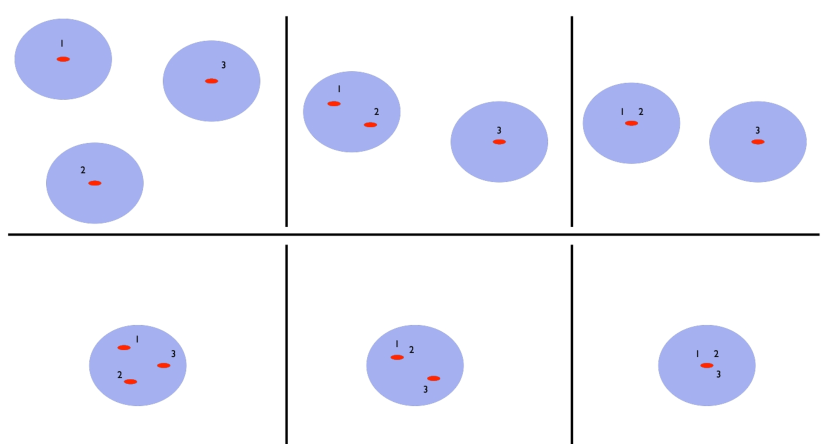
Figure 6: Diagrams for the 3D galaxy bispectrum. From left to right and top to bottom : (3-halo), (2-halo 3-galaxies), (2-halo 2-galaxies), (1-halo 3-galaxies), (1-halo 2-galaxies), (1-halo 3-galaxies).

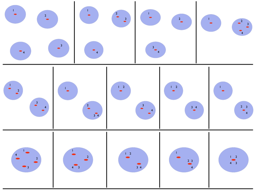
Figure 7: Diagrams for the 3D galaxy trispectrum

We described in the previous sections the mass function, halo profile and the HOD governing the number of galaxies in a halo. The final element needed for the computation of the galaxy polyspectra is a description of the halo polyspectra. To this end, we adopt the local biasing scheme which allows to compute the halo polyspectrum from the matter polyspectrum as described in Appendix C.

At high order, the halo polyspectrum has thus several possible sources. The first source is the first order biasing of the corresponding dark matter polyspectrum, either primordial (primordial non-Gaussianity) or from perturbation theory. In the bispectrum case, it produces the 3hcos term. The second source is the higher order biasing of lower order dark matter polyspectrum. In the bispectrum case, it produces the 3h term.

Hence, we have proposed a diagrammatic method to compute galaxy polyspectra which gives the power and simplicity of drawings to compute otherwise cumbersome equations at high order. The focus of the next section is to relate these 3D polyspectra to observables on the sky.

4 CIB angular polyspectra on the sky

Measurements of the CIB clustering are carried out on the celestial sphere. Hence a statistical characterisation of random fields on the sphere is needed, as well as the projection of the statistics of 3D random fields onto the sphere.
In this section, we first describe the formalism of correlation functions on the sphere, then we derive the CIB angular polyspectrum. Eventually, we discuss the shot noise terms and the effect of the flux cut.

4.1 Correlation functions in harmonic space

Given a full-sky map of the temperature $T(\hat{n})$ of some signal on the celestial sphere, it can be decomposed in the harmonic basis as

$$T(\hat{n})=\sum_{\ell m}a_{\ell m}\,Y_{\ell m}(\hat{n})$$ (28)

with

$$a_{\ell m}=\int\mathrm{d}^{2}\hat{n}\;Y^{*}_{\ell m}(\hat{n})\;\Delta T(\hat{n})$$ (29)

with the usual orthonormal spherical harmonics $Y_{\ell m}$.
For a –statistically isotropic– Gaussian field, all the statistical information is contained in the power spectrum $C_{\ell}$, the 2-point correlation function in harmonic space: $\langle a_{\ell m}\,a^{*}_{\ell^{\prime}m^{\prime}}\rangle=C_{\ell}\,\delta_{\ell\ell^{\prime}}\,\delta_{mm^{\prime}}$. For non-Gaussian fields, information is also contained in higher-order moments. For instance, the bispectrum $b_{\ell_{1}\ell_{2}\ell_{3}}$ is:

$$\langle a_{\ell_{1}m_{1}}a_{\ell_{2}m_{2}}a_{\ell_{3}m_{3}}\rangle=G_{\ell_{1}\ell_{2}\ell_{3}}^{m_{1}m_{2}m_{3}}\times b_{\ell_{1}\ell_{2}\ell_{3}}$$ (30)

with the Gaunt coefficient

$$G_{1,2,3} =\int\mathrm{d}^{2}\hat{n}\;Y_{123}(\hat{n})$$ (31)

$$=\sqrt{\frac{(2\ell+1)_{123}}{4\pi}}\left(\begin{array}[]{ccc}\ell_{1}&\ell_{2}&\ell_{3}\\ 0&0&0\end{array}\right)\left(\begin{array}[]{ccc}\ell_{1}&\ell_{2}&\ell_{3}\\ m_{1}&m_{2}&m_{3}\end{array}\right)$$ (36)

where $Y_{i}=Y_{\ell_{i}m_{i}}$. In the following, the subscript 123 denotes the product of the corresponding variables, e.g., $X_{123}\equiv X_{1}\,X_{2}\,X_{3}$. The Gaunt coefficient is zero unless the triplet $(\ell_{1},\ell_{2},\ell_{3})$ follows the triangle inequalities and $m_{1}+m_{2}+m_{3}=0$.

Higher order polyspectra $\mathcal{P}^{(n)}(\ell_{1\cdots n}\,,\ell^{\mathrm{d}}_{1\cdots(n-3)})$ are defined in Appendix D, along with the case of diagonal independence.

The one-to-one correspondence between the full pdf and the hierarchy of polyspectra for $n$ up to infinity ensures that the polyspectra provide us with a full statistical characterisation of a given field on the sphere.

4.2 Anisotropy projection on the sky

The CIB is mostly unresolved in the far-infrared domain which leads to the loss of the redshift information. The emission is thus integrated on a large range of redshift ($1<z<4$), and the CIB temperature in a given direction $\hat{n}$, is a line-of-sight integral of the IR emissivity j_ν per comoving volume:

$$T(\hat{n},\nu)=\int\mathrm{d}z\,\frac{\mathrm{d}r}{\mathrm{d}z}\,a(z)\,\texttt{j}_{\nu}\left(r(z)\,\hat{n},z\right)$$ (37)

with j_ν in Jy/Mpc so that $T$ has units of Jy/sr and may be converted to a temperature elevation at CMB frequencies through Planck’s law. Here $r$ is the comoving distance to redshift $z$ and $a$ is the scale factor.
Using the Rayleigh/plane wave expansion and the Fourier expansion of the emissivity field, we obtain:

$$a_{\ell m}(\nu)=i^{\ell}\int\frac{\mathrm{d}^{3}\mathbf{k}}{2\pi^{2}}\,\mathrm{d}z\,\frac{\mathrm{d}r}{\mathrm{d}z}\,a(z)\,j_{\ell}(kr)\,Y^{*}_{\ell m}(\hat{k})\,\texttt{j}_{\nu}(\mathbf{k},z)$$ (38)

where $j_{\ell}$ is the spherical Bessel function of order $\ell$.

We relate in Appendix E the CIB angular polyspectrum to the 3D emissivity polyspectra, for the terms which are diagonal-independent. This gives:

$$\mathcal{P}^{(n)}_{\mathrm{CIB}}(\ell_{1},\cdots,\ell_{n}) =\left(\frac{2}{\pi}\right)^{n}\!\!\int\!k^{2}_{1\cdots n}\mathrm{d}k_{1\cdots n}\,\mathrm{d}z_{1\cdots n}\,x^{2}\mathrm{d}x$$

$$\left[a(z_{i})\left.\frac{\mathrm{d}r}{\mathrm{d}z}\right|_{z_{i}}\,j_{\ell_{i}}(k_{i}r_{i})j_{\ell_{i}}(k_{i}x)\right]_{i=1\cdots n}$$

$$\qquad\times\mathcal{P}^{(n)}_{\texttt{j}}(k_{1\cdots n},z_{1\cdots n})$$ (39)

with parity invariance imposing $\ell_{1}+\cdots+\ell_{n}$ to be even.
In the Limber’s approximation, Eq.39 simplifies to :

$$\mathcal{P}^{(n)}_{\mathrm{CIB}}(\ell_{1},\cdots,\ell_{n})=\int\frac{r^{2}\mathrm{d}r}{r^{2n}}a^{n}(z)\,\mathcal{P}^{(n)}_{\texttt{j}}(k^{*}_{1\cdots n},z)$$ (40)

with $k^{*}=(\ell+1/2)/r(z)$. Note that, as a consequence of Limber’s approximation, Eq.40 now involves the emissivity polyspectrum at a single redshift (i.e., $z_{1}=\cdots=z_{n}=z$).

Galaxy power spectrum and galaxy emissivity are often related assuming implicitly or explicitly that all galaxies at a given redshift $z$ have the same luminosity (e.g., Knox et al., 2001; Pénin et al., 2012; Xia et al., 2012). We will refer to this approach as the constant-luminosity assumption. It yields :

$$\delta\texttt{j}_{\nu}(\mathbf{k},z)=\overline{\texttt{j}}_{\nu}(z)\cdot\delta_{\mathrm{gal}}(\mathbf{k},z)$$ (41)

where the average emissivity $\overline{\texttt{j}}_{\nu}$ is computed from galaxy number counts.
In the present study, we propose a more general assumption referred to as the flux-abundance independence assumption. That is, we assume that the flux is stochastic with a distribution given by the number counts, and furthermore that the stochasticity is independent of the galaxy position/abundance. The commonly used constant-luminosity assumption is a special case of the flux-abundance independence assumption when the luminosity function $\frac{\mathrm{d}^{2}N}{\mathrm{d}L\,\mathrm{d}V}$ is a dirac. Note that, although the flux-abundance independence is a more general assumption than the constant luminosity one, it does not capture the possibility that the luminosity may depend on underlying variables having an influence on galaxy abundance (e.g., the host halo mass).

For non shot-noise terms, the flux-abundance independence assumption yields the same relation as the constant-luminosity assumption:

$$\mathcal{P}^{(n)}_{\texttt{j}}(k^{*}_{1\cdots n},z)=\overline{\texttt{j}}_{\nu}(z)^{n}\ \mathcal{P}^{(n)}_{\mathrm{gal}}(k^{*}_{1\cdots n},z).$$ (42)

The difference between the two assumptions impacts the shot-noise terms as discussed in detail in Sect.4.3.

For non shot-noise terms, the angular polyspectrum then takes the form :

$$\mathcal{P}^{(n)}_{\mathrm{CIB}}(\ell_{1},\cdots,\ell_{n})=\int\frac{\mathrm{d}z}{r^{2n-2}}\,\frac{\mathrm{d}r}{\mathrm{d}z}\,a^{n}(z)\,\overline{\texttt{j}}_{\nu}(z)^{n}\,\mathcal{P}^{(n)}_{\mathrm{gal}}(k^{*}_{1\cdots n},z)$$ (43)

In particular at second order the power spectrum is

$$C_{\ell}(\nu)=\int\frac{\mathrm{d}z}{r^{2}}\,\frac{\mathrm{d}r}{\mathrm{d}z}\,a^{2}(z)\,\overline{\texttt{j}}_{\nu}^{\,2}(z)\,P_{\mathrm{gal}}(k^{*},z)$$ (44)

as given e.g. by Knox et al. (2001); Pénin et al. (2012); Xia et al. (2012)
And at third order, the bispectrum is

$$b_{\ell_{1}\ell_{2}\ell_{3}}=\int\frac{\mathrm{d}z}{r^{4}}\,\frac{\mathrm{d}r}{\mathrm{d}z}\,a^{3}(z)\,\overline{\texttt{j}}_{\nu}^{3}(z)\,B_{\mathrm{gal}}(k^{*}_{123},z)$$ (45)

4.3 Shot-noise

The shot-noise terms, for the power spectrum or for the bispectrum, correspond to terms in the correlation function involving multiple times the same galaxy. For the power spectrum, the halo model gives the galaxy shot-noise power spectrum :

$$P_{\mathrm{gal}}^{\mathrm{shot}}(k,z)=\frac{1}{\overline{n}_{\mathrm{gal}}(z)}$$ (46)

With the constant-emissivity assumption, we get the angular power spectrum :

$$C_{\ell}^{\mathrm{shot}}=\int_{z=0}^{\infty}\frac{\mathrm{d}z}{r^{2}}\,\frac{\mathrm{d}r}{\mathrm{d}z}\,a^{2}(z)\,\overline{\texttt{j}}_{\nu}^{2}(z)\,P_{\mathrm{shot}}(k,z)$$ (47)

The shot-noise level can be predicted from number counts (see e.g., Lacasa et al., 2012) as :

$$C_{\ell}^{\mathrm{shot}}=\int_{z=0}^{\infty}\int_{0}^{S_{\mathrm{cut}}}S^{2}\,\frac{\mathrm{d}^{2}n}{\mathrm{d}S\,\mathrm{d}z}\,\mathrm{d}S\,\mathrm{d}z$$ (48)

These two formula agree if indeed all sources have the same luminosity, potentially depending on redshift. However in reality, sources do not have the same luminosity ; and specifically Eq.48 will give more weight to bright galaxies –averaging $S^{2}$– as compared to Eq.47 –averaging $S$.
With the flux-abundance independence assumption, the distribution of luminosities can be incorporated in the model by introducing the nth-order emissivities :

$$\texttt{j}_{\nu}^{(n)}(z)=\frac{(1+z)^{n}\;r(z)^{2n-2}}{\frac{\mathrm{d}r}{\mathrm{d}z}}\int_{0}^{S_{\mathrm{cut}}}S^{n}\frac{\mathrm{d}^{2}N}{\mathrm{d}S\,\mathrm{d}z}\mathrm{d}S$$ (49)

which effectively average $S^{n}$ instead of $S$. Removing $\overline{n}_{\mathrm{gal}}(z)$ factors from the shot-noise 3D power spectrum, the shot-noise angular power spectrum becomes :

$$C_{\ell}^{\mathrm{shot}}=\int\frac{\mathrm{d}z}{r^{2}}\,\frac{\mathrm{d}r}{\mathrm{d}z}\,a^{2}(z)\,\texttt{j}_{\nu}^{(2)}(z)\times 1$$ (50)

which can be shown to be equivalent to Eq.48.

At any order, with the diagrammatic approach described in Sect.3.2, the shot noise terms can be computed and integrated over redshifts with Eq.43 provided the following modification :
For each contraction, $\texttt{j}_{\nu}^{p}(z)/\overline{n}_{\mathrm{gal}}^{\,p-1}$ must be replaced by the $p$-th order emissivity $\texttt{j}_{\nu}^{(p)}(z)$, where $p$ is the order of the contraction under consideration.

For example for the bispectrum, the 3D shot-noise contains three terms (see Appendix B) :

$$B^{\mathrm{shot}}_{\mathrm{gal}}(k_{1},k_{2},k_{3},z)=B^{\mathrm{1h-1g}}_{\mathrm{gal}}+B^{\mathrm{1h-2g}}_{\mathrm{gal}}+B^{\mathrm{2h-2g}}_{\mathrm{gal}}$$ (51)

with

$$B^{\mathrm{1h-1g}}_{\mathrm{gal}}(k_{1},k_{2},k_{3},z) =\frac{1}{\overline{n}_{\mathrm{gal}}^{2}(z)}$$ (52)

$$B^{\mathrm{1h-2g}}_{\mathrm{gal}}(k_{1},k_{2},k_{3},z) =\frac{P^{\mathrm{1h-2g}}_{\mathrm{gal}}(k_{1})+P^{\mathrm{1h-2g}}_{\mathrm{gal}}(k_{2})+P^{\mathrm{1h-2g}}_{\mathrm{gal}}(k_{3})}{\overline{n}_{\mathrm{gal}}(z)}$$ (53)

$$B^{\mathrm{2h-2g}}_{\mathrm{gal}}(k_{1},k_{2},k_{3},z) =\frac{P^{\mathrm{2h-2g}}_{\mathrm{gal}}(k_{1})+P^{\mathrm{2h-2g}}_{\mathrm{gal}}(k_{2})+P^{\mathrm{2h-2g}}_{\mathrm{gal}}(k_{3})}{\overline{n}_{\mathrm{gal}}(z)}$$ (54)

Now taking into account luminosity distribution, the 1-galaxy angular shot-noise takes the form :

$$b_{\ell_{123}}^{\mathrm{shot1g}}=\int\frac{\mathrm{d}z}{r^{4}}\,\frac{\mathrm{d}r}{\mathrm{d}z}\,a^{3}(z)\,\texttt{j}_{\nu}^{(3)}(z)\times 1$$ (55)

And the 2-galaxy shot-noise :

$$b_{\ell_{123}}^{\mathrm{shot2g}} =\int\frac{\mathrm{d}z}{r^{4}}\,\frac{\mathrm{d}r}{\mathrm{d}z}\,a^{3}(z)\,\texttt{j}_{\nu}^{(1)}(z)\;\texttt{j}_{\nu}^{(2)}(z)$$

$$\times\left[P^{\mathrm{clust}}_{\mathrm{gal}}(k^{*}_{1})+P^{\mathrm{clust}}_{\mathrm{gal}}(k^{*}_{2})+P^{\mathrm{clust}}_{\mathrm{gal}}(k^{*}_{3})\right]$$ (56)

with $P^{\mathrm{clust}}_{\mathrm{gal}}(k)=P^{\mathrm{1h}}_{\mathrm{gal}}(k,z)+P^{\mathrm{2h}}_{\mathrm{gal}}(k,z)$, and as usual $k^{*}~{}=~{}\frac{\ell+1/2}{r(z)}$.

In this formulation, the flux cut, or more generally the selection function, is implemented in the $p$-order emissivities. The shot-noise terms are quite sensitive to the value of this flux limit, which in turn depends on the instrumental setup used for the observation. Hence, the amplitude of the shot-noise terms may change depending on the instrument considered.

4.4 Flux cut and low redshift contribution

As can be seen on Eq.50 and 55, the shot-noise equations diverge if the emissivities tend to a constant as $z\rightarrow 0$. This is indeed the case in the Euclidean case ($\frac{\mathrm{d}n}{\mathrm{d}S}\propto S^{-5/2}$) where Eq.48 diverges if no flux cut is applied.

In practice, the flux cut reduces the contribution from low redshift sources which dominate the counts. This needs to be reflected in the halo model, where the number of objects is dictated by the HOD. For simplicity, we implement the flux cut in terms of a cut-off in the redshift integrals at $z_{\mathrm{cut}}$. Below this redshift, a typical galaxy with luminosity $L_{*}$ (the knee of the luminosity function) has a flux $S\geq S_{\mathrm{cut}}$ :

$$S_{\mathrm{cut}}=\frac{L_{*}}{4\pi\,d^{2}_{L}(z_{\mathrm{cut}})}$$ (57)

with $d_{L}$ the luminosity distance.
The effect of the flux cut on the galaxy clustering has not been considered previously in the CIB power spectrum literature, although it is theoretically necessary. We found that it has a small effect on the power spectrum, mostly on the 1-halo term and for some values of the HOD parameters ($\alpha>1$). The redshift cut has more effect on the bispectrum and potentially at higher order, as they may be more sensitive to low redshift because of the $r(z)^{2n-2}$ denominator in Eq.43 which goes to zero as $z\rightarrow 0$.

5 Results

5.1 The CIB angular bispectrum

In the following, we apply our formalism to the computation of the bispectrum of the CIB. To this end, the HOD best-fit parameters were obtained so as to reproduce CIB power spectrum constraints (Pénin et al., 2013). We also use the galaxy emission model by Béthermin et al. (2011) at 350 $\mu$m = 857 GHz with a flux cut at 0.82 Jy (Planck Collaboration et al., 2011b), which implies a redshift cut at $z_{\mathrm{cut}}=0.03$.

The obtained CIB bispectrum and its different terms are displayed in Fig.8 in some particular configurations : equilateral, orthogonal isoceles, flat isoceles and squeezed. We consider a multipole range of $\ell=30-2000$. On this range of scales, shot-noise terms are found to be negligible, as happens for the power spectrum (Pénin et al., 2012). However, they are expected to dominate on smaller scales ($\ell\sim 5000$ for the particular galaxy emission model used in the present study). The 2-halo and 3-halo terms dominate on large scales $\ell\leq 300$, while the 1-halo dominates on small scales, except in the squeezed configuration where the 2-halo term dominates for $\ell>300$.

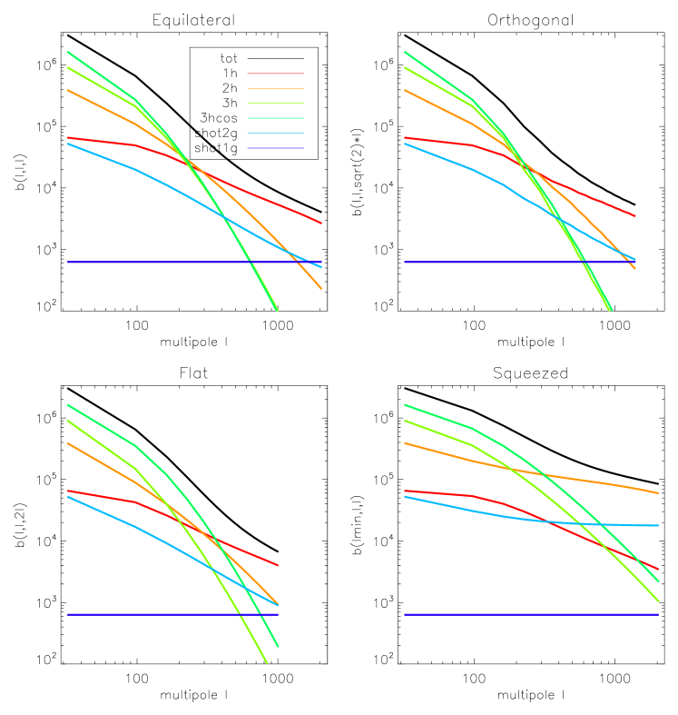
Figure 8: CIB bispectrum and its different terms in some particular configurations at 350 $\mu$m = 857 GHz. The squeezed configuration uses $\ell_{\mathrm{min}}=32$.

An interesting point is the configuration dependence of the bispectrum. Figure 9 shows the CIB bispectrum at 350 $\mu$m plotted in the geometrical parametrisation proposed in Lacasa et al. (2012). The values of the bispectrum are color-coded from violet to red. In this parametrisation, each subplot shows a slice of the bispectrum at a given perimeter, indicated in the bottom left corner. All triangles within the perimeter bin are shown in the subplot, with squeezed triangles in the upper left corner, equilateral triangle in the upper right corner and flat isosceles triangle in the bottom corner. The geometrical parametrisation permits us to visualise, at the same time, both the scale and configuration dependence of the bispectrum. We do not display the 1-galaxy shot-noise term since it is constant.

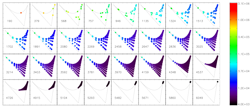
Figure 9: CIB bispectrum in the geometrical parametrisation at 350 $\mu$m = 857 GHz. It exhibits a peak in the squeezed configurations (upper left corner of each subplot).

As seen already in Fig.8, the CIB bispectrum decreases generally with scale, as it is the case for the power spectrum. A distinctive feature of the CIB bispectrum is that it peaks in the squeezed configuration, as already noted by Lacasa et al. (2012). Figures 10–14 show the different terms of the CIB bispectrum plotted in the geometrical parametrisation with the color range adapted to each term to highlight its variations.

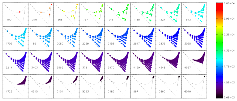
Figure 10: The 1-halo term of the CIB bispectrum in the geometrical parametrisation at 350 $\mu$m = 857 GHz. It has strong scale dependence but few dependence on configuration.

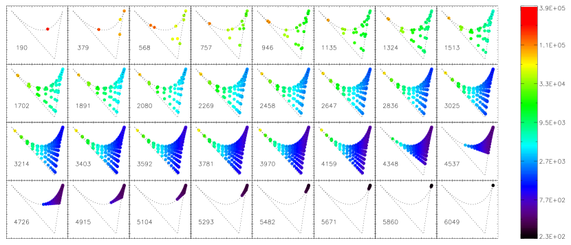
Figure 11: The 2-halo term of the CIB bispectrum in the geometrical parametrisation at 350 $\mu$m = 857 GHz. It exhibits a peak in the squeezed configurations (upper left corner of each subplot).

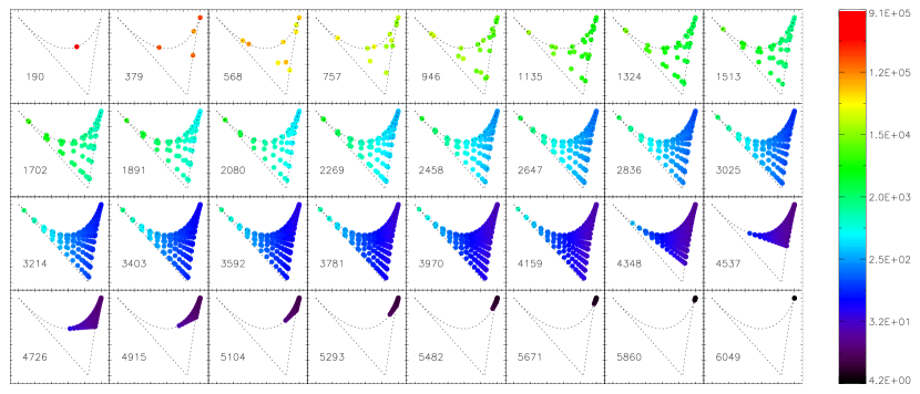
Figure 12: The 3-halo term of the CIB bispectrum in the geometrical parametrisation at 350 $\mu$m = 857 GHz. It exhibits a peak in the squeezed configurations (upper left corner of each subplot).

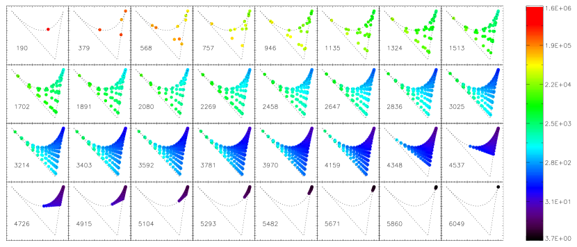
Figure 13: The 3-halo cos term of the CIB bispectrum in the geometrical parametrisation at 350 $\mu$m = 857 GHz. It exhibits a peak in the squeezed configurations (upper left corner of each subplot), and in the flat configurations (down corner of each subplot) for some perimeter bins.

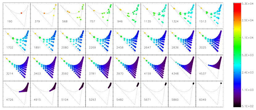
Figure 14: 2-galaxy shot-noise term of the CIB bispectrum in the geometrical parametrisation at 350 $\mu$m = 857 GHz. It exhibits a peak in the squeezed configurations (upper left corner of each subplot).

It is worth noting that most terms peak strongly in the squeezed configurations, except the 1-halo term. The latter has little configuration dependence but strong scale dependence and is slightly weaker in squeezed. The 3hcos term from perturbation theory is, unlike other terms, more important in the flat configuration than in the equilateral. This is due to the $F^{s}$ kernel (Eq.23) which is more important in flat than in equilateral configurations.

5.2 Dependencies on the HOD parameters

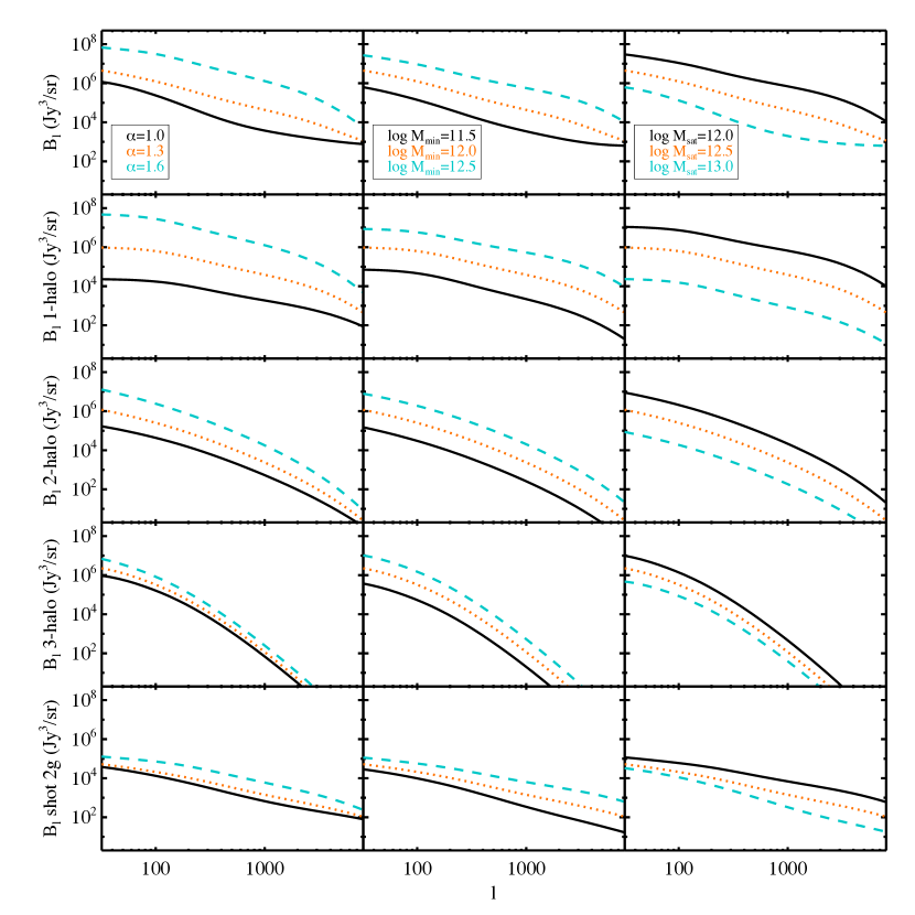
Figure 15: Equilateral bispectra at 350 $\mu$m  for several sets of the HOD parameters. Only one parameter is varied while the others keep their fiducial values.

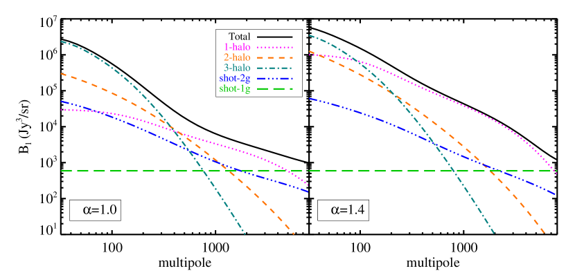
Figure 16: Equilateral bispectrum at 350 $\mu$m  with $\alpha_{\mathrm{sat}}$=1 and $\alpha_{\mathrm{sat}}$=1.4. The other HOD parameters are fixed at their fiducial values.

We now investigate how the bispectrum and its different components vary with respect to the HOD parameters. We use a fiducial set of HOD parameters inspired from previous studies of CIB anisotropies, namely (Viero et al., 2009; Amblard et al., 2011; Planck Collaboration et al., 2011a), and we vary them individually. Only one parameter is varied, by typically $2\sigma$ (for instance, Planck Collaboration et al., 2011a), while the others keep their fiducial values. We consider $\alpha_{\mathrm{sat}}$=1.3, $\log$ $M_{\mathrm{min}}$= 12, $M_{\mathrm{sat}}$= 10 $M_{\mathrm{min}}$ and $\sigma_{\mathrm{\log M}}$= 0.65. As a reminder, increasing (decreasing) $\alpha_{\mathrm{sat}}$ leads to a higher (lower) number of satellite galaxies. The value of $M_{\mathrm{min}}$ rules the mass at which a halo contains a central galaxy and $M_{\mathrm{sat}}$ is the average mass of a halo hosting satellite galaxies.

Figure 15 displays the equilateral bispectrum at 350 $\mu$m  and its components. We do not display the 1-galaxy shot noise term as it is independent of the HOD parameters. First, we see that the amplitude of each component of the bispectrum is very sensitive to the value of each HOD parameter. Indeed, the amplitude can increase/decrease by up to two orders of magnitude. For instance, a higher $\alpha_{\mathrm{sat}}$ leads to more power at all scales as it means more satellite galaxies as compared to a lower $\alpha_{\mathrm{sat}}$. The shape of the bispectrum terms only varies slightly with the HOD parameters. Furthermore, variations of different parameters induce similar changes on the equilateral bispectrum suggesting a degeneracies between the HOD parameters. The degeneracy and how it could be broken are discussed in Paper2.
It is interesting to notice that $\alpha_{\mathrm{sat}}$ induces strong variations in the relative contributions of each term of the bispectrum. Fig. 16 shows each component of the bispectrum for two values of $\alpha_{\mathrm{sat}}$. For $\alpha_{\mathrm{sat}}$=1.4 the 1-halo term dominates all the other contributions on nearly all angular scales. The bispectrum thus appears much more sensitive to $\alpha_{\mathrm{sat}}$ than the power spectrum. This effect might help to alleviate the tension that exists today about the measured values of $\alpha_{\mathrm{sat}}$ (see Paper2).

5.3 Halos contribution

We can now focus on halo contribution to the 3D galaxy bispectrum. Most terms, except the 1-halo term, are not a simple integration over halo mass, but include cross-terms between halos of different masses. The 3D galaxy bispectrum cannot be simply divided into a sum of contributions of different mass bins. We may focus on the dependence of the bispectrum on the halo-mass upper cut-off. In Fig.17, we display the total 3D galaxy bispectrum in the equilateral configuration, as a function of the halo-mass upper cut-off, respectively at $z$=0.1 and $z$=1.

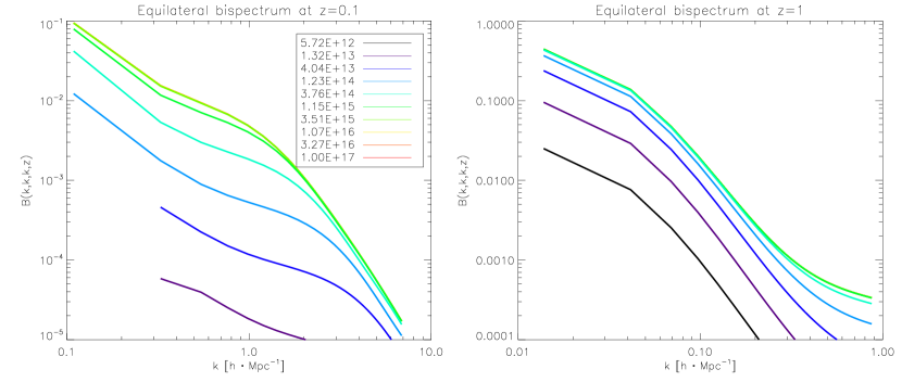
Figure 17: Total galaxy equilateral bispectrum at redshift 0.1 and 1, as a function of the halo mass upper cut-off from $M_{\mathrm{cut}}=5.7\,10^{12}M_{\odot}$ to $10^{17}M_{\odot}$.

At $z$=1, we see that the equilateral bispectrum saturates for a cut-off at a few $10^{14}\,\mathrm{M}_{\odot}$, except at small scales where saturation is reached for $\sim 10^{15}\,\mathrm{M}_{\odot}$. So at this redshift, halos with masses larger than a few $10^{15}\,\mathrm{M}_{\odot}$ contribute negligibly to the bispectrum, as there are too few of them. At $z$=0.1, massive halos contribute more importantly to the bispectrum, which saturates at a cut-off $\sim 10^{15}\,\mathrm{M}_{\odot}$ on small scales and at $\sim 4\!\times\!10^{15}\,\mathrm{M}_{\odot}$ on large scales. This reflects also the increase in number of massive halos at low redshift.

We checked each of the bispectrum terms and found that the 1-halo term is the most sensitive to massive halos, while the 3-halo terms (both 3h and 3hcos) are the least sensitive, saturating at a few $10^{14}\,\mathrm{M}_{\odot}$ even at low redshift. This behaviour is expected since the 3-halo terms involve the product of three halo mass functions. This penalises massive halos in the tail of the mass function as there are few of them. On the contrary, the 1-halo term involves only one mass function, and it gives more weight to massive halos containing more galaxies (see $N_{\mathrm{gal}}(M)^{3}$ weight).

The mass contribution to the angular bispectrum depends on the galaxy emissivities which give weights to each redshift. It hence depends on the specific galaxy evolution model chosen. This is discussed in details in the companion article (Pénin et al., 2013, paper2)

6 Discussion

6.1 Comparison with empirical prescription

A simple empirical prescription for the CIB bispectrum based on its power spectrum was proposed by Lacasa et al. (2012). It reads :

$$b_{123}^{\mathrm{CIB}}=\alpha\,\sqrt{C_{\ell_{1}}^{\mathrm{CIB}}\,C_{\ell_{2}}^{\mathrm{CIB}}\,C_{\ell_{3}}^{\mathrm{CIB}}}$$ (58)

where $\alpha$ is a proportionality constant that can be computed with the number counts of IR galaxies and their flux cut.

We compare this prescription with the CIB bispectrum obtained from the halo model theory. For the prescription, we used the CIB power spectrum predicted by the halo model with the same parameters as for the bispectrum, and the best-fit value $\alpha=2.25\times 10^{-3}$ (compared to $\alpha=3\times 10^{-3}$ found by Lacasa et al. 2012 on simulations by Sehgal et al. 2010). Figure 18 shows both bispectra at 350 $\mu$m (the prescription is in red and the halo model in black).

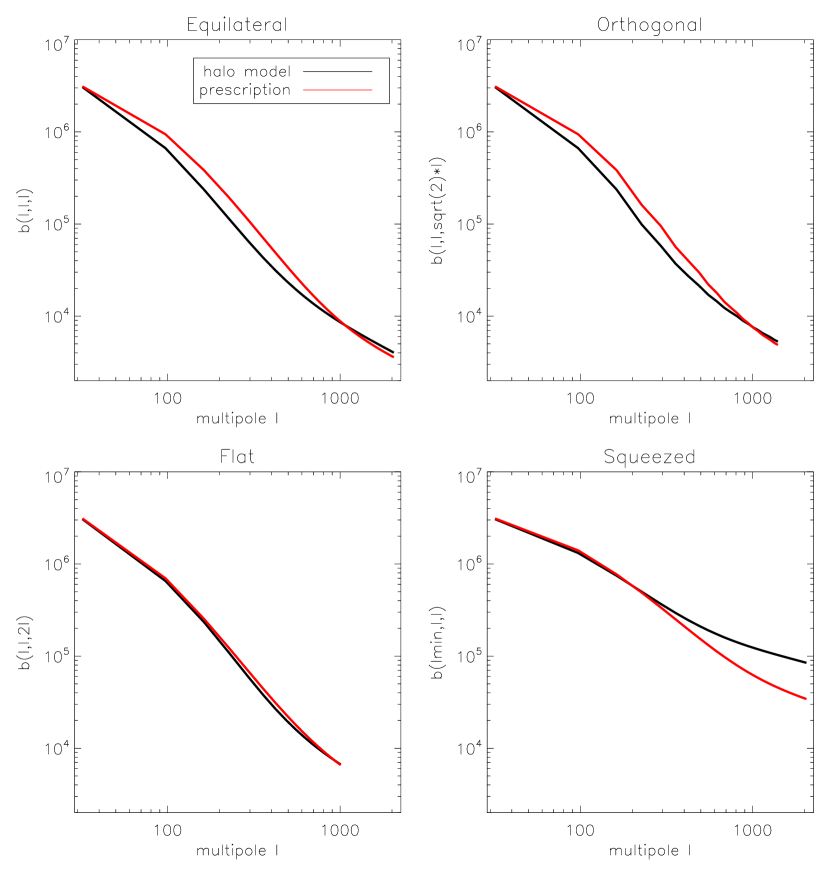
Figure 18: CIB bispectrum computed with the halo model (black line) and with the prescription (red line) at 350 $\mu$m

We see that the prescription reproduces reasonably well the shape of the bispectrum in equilateral, orthogonal and flat configurations. However, the empirical prescription shows an excess of power at intermediate multipoles $\ell\in[100,1000]$ in the equilateral and isosceles orthogonal configurations. Finally, the prescription does not recover the bispectrum in the squeezed configuration, departing from the halo model at $\ell\sim 300$, i.e. when the 2-halo term begins to dominate the squeezed bispectrum (see Fig.8).

The empirical prescription therefore gives a reasonable overall fit of the CIB bispectrum, for the considered galaxy emission model and HOD parameters. Furthermore, the prescription gives a separable template (i.e., $b_{123}=f(\ell_{1})f(\ell_{2})f(\ell_{3})$ for some function $f$) ; it thus provides a convenient way to assess quickly the overall level of CIB non-gaussianity present in a CMB map. This is useful in particular to assess the level of contamination of $f_{\mathrm{NL}}$ estimation (see Lacasa & Aghanim, 2012). Nevertheless, the empirical prescription does not reproduce completely the theoretical bispectrum derived from the halo model. Additionally in the companion article (Paper2), we show that galaxy evolution models which are indistinguishable at the power spectrum level can produce distinguishable theoretical bispectra with the halo model. On the contrary, for different galaxy models the empirical prescription would give indistinguishable bispectra, as it is based on the power spectra. A full computation of the bispectrum using the halo model is thus necessary if one were to interpret a CIB non-Gaussianity measurement.

6.2 Comparison with radio sources and CMB bispectra

At microwave frequencies, several extragalactic signals other than the CIB are present. In particular, the CMB and radio sources which emit mostly at low frequencies, $\nu\leq$ 217 GHz (Planck Collaboration, 2012). We thus compare the bispectra of those extragalactic signals with the CIB theoretical bispectrum derived from the halo model.

Radio sources can be considered distributed randomly on the sky (Toffolatti et al., 1998), at least for the brightest sources. Hence, the extragalactic radio background has a white-noise distribution entirely characterised by the number counts $\frac{\mathrm{d}N}{\mathrm{d}S}$. The expected power spectrum and bispectrum is :

$$C_{\ell}^{\mathrm{RAD}} = \int_{0}^{S_{\mathrm{cut}}}S^{2}\,\frac{\mathrm{d}N}{\mathrm{d}S}\,\mathrm{d}S$$ (59)

$$b_{\ell_{1}\ell_{2}\ell_{3}}^{\mathrm{RAD}} = \int_{0}^{S_{\mathrm{cut}}}S^{3}\,\frac{\mathrm{d}N}{\mathrm{d}S}\,\mathrm{d}S$$ (60)

in Jy²/sr and Jy³/sr² respectively, with $\frac{\mathrm{d}N}{\mathrm{d}S}$ in gal/Jy/sr and $S_{\mathrm{cut}}$ the flux cut. The radio bispectrum is hence flat, with neither scale nor geometrical dependence.
In the following, we use number counts from Tucci et al. (2011), and flux cuts from Planck Collaboration et al. (2011b).

In the standard paradigm, inflation generates close to Gaussian perturbations which evolve to Gaussian-distributed temperature fluctuations of the CMB. In the last decade, interest has increased for the search of CMB non-Gaussianity (e.g., Komatsu et al., 2011), as it would be a signature of non-standard inflation (violating any of the following assumption : slow-roll single-field inflation with standard kinetic term and Bunch-Davies initial condition, see Bartolo et al., 2004, for a review), or any physical process generating the primordial perturbations, or of non-linear evolution (e.g., Pitrou et al., 2010). With the recent Planck measurements, the CMB appears to be very close to a Gaussian field (Planck Collaboration XXIV, 2013).

Among the many primordial non-Gaussianity shapes, the most studied is the ‘local’ non-Gaussianity factor $f_{\mathrm{NL}}$, where the Bardeen potential takes the form (Komatsu & Spergel, 2001) :

$$\Phi(\mathbf{x})=\Phi_{G}(\mathbf{x})+f_{\mathrm{NL}}\cdot(\Phi_{G}(\mathbf{x})^{2}-\langle\Phi_{G}(\mathbf{x})^{2}\rangle)$$ (61)

with $\Phi_{G}$ the Gaussian part of the potential. This primordial non-Gaussianity generates a CMB bispectrum of the form (Komatsu et al., 2005) :

$$b_{\ell_{1}\ell_{2}\ell_{3}}^{\mathrm{CMB}}=f_{\mathrm{NL}}\int r^{2}\mathrm{d}r\;\alpha_{\ell_{1}}(r)\,\beta_{\ell_{2}}(r)\,\beta_{\ell_{3}}(r)+\mathrm{perm.}$$ (62)

with an integral along the line-of-sight, and filters :

$$\alpha_{\ell}(r) = \frac{2}{\pi}\int k^{2}\mathrm{d}k\,g_{T,\ell}(k)\,j_{\ell}(kr)$$ (63)

$$\beta_{\ell}(r) = \frac{2}{\pi}\int k^{2}\mathrm{d}k\,P(k)\,g_{T,\ell}(k)\,j_{\ell}(kr)$$ (64)

where $g_{T,\ell}$ is the radiation transfer function, which can be computed with a Boltzmann code, and $P(k)\propto k^{n_{s}-4}$ is the primordial power spectrum, with a spectral index $n_{s}$.
The CMB physics, e.g. acoustic peaks and Silk damping, is encoded into its bispectrum thanks to the radiation transfer function.

We show, in Fig.19, the bispectra of radio sources and the CMB for $f_{\mathrm{NL}}=1$ together with the CIB bispectrum derived from the halo model, in units of relative temperature elevation $\Delta T/T$, at 1380 $\mu$m = 220 GHz. At this frequency, radio and infrared point-sources have comparable contributions, whereas radio sources dominate at lower frequencies and infrared sources dominate at higher frequencies.

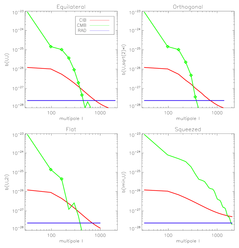
Figure 19: CIB (red line), radio (blue line) and CMB (green line) bispectra at 220 GHz in dimensionless units $\Delta T/T$. The latter is for $f_{\mathrm{NL}}=1$, and we plot its absolute value as it is mostly negative, diamond indicate positive points.

We see that the CMB dominates on large angular scales, but plummets at high multipoles and becomes negligible for $\ell\geq 500$, except in the squeezed configuration where the CMB dominates at all scales. Indeed for local type non-Gaussianity, the CMB bispectrum peaks strongly in the squeezed limit (Bucher et al., 2010). The CIB bispectrum also peaks on large angular scales, albeit less strongly than the CMB. It dominates the radio bispectrum up to $\ell\sim 700-800$ and becomes negligible afterwards except in the squeezed limit where it dominates the radio over the whole multipole range. Based on this simple comparison, it seems that detecting the CIB bispectrum can be possible above 220 GHz. At 220 GHz, if most of the CMB can be removed by a component separation method (which estimates a CMB map through multifrequency analysis, see Delabrouille & Cardoso, 2007, for a review), the detection of the CIB bispectrum is possible at $\ell\leq 700$. Furthermore, the application of a lower flux cut would lower the level of the radio bispectrum and uncover the CIB one. For instance, the CIB bispectrum has been detected in the South Pole Telescope data in a multifrequency analysis using 95, 150 and 220 GHz channels (Crawford et al., 2013), and in the Planck data with a signal-to-noise ratio S/N=5.8 at 217 GHz (Planck Collaboration et al., 2013).

7 Conclusion

We have presented a framework which allows to predict galaxy clustering at all orders with the halo model including shot-noise consistently. We have developed a new diagrammatic method which allows a clear representation and understanding of the different terms involved in the computation of the 3D galaxy polyspectrum. It further allows to avoid cumbersome computation at high orders by replacing them with diagram drawings. This diagrammatic framework is adaptable to different galaxy-tracing signals and we apply it to the CIB. The latter being integrated over a large range of redshift, we show how the polyspectrum of the CIB anisotropies is projected on the celestial sphere. We further show how to account for the particular case of the shot-noise terms.
This framework allows us to compute the CIB angular bispectra at any frequency. We have investigated how the different terms of the resulting CIB bispectrum depend on the scale and on the triangle configuration. We recover that the total bispectrum peaks in the squeezed limit as it is also the case for primordial non-Gaussianity of the local-type. We discuss how the terms of the CIB bispectrum vary with the halo occupation distribution parameters. We show that they vary similarly with respect to the different HOD parameters indicating degeneracies. Furthermore, we show that the bispectrum is much more sensitive to the variation of these parameters than the power spectrum.
We explore the halo mass contribution to each term of the 3D galaxy bispectrum, recovering that the 1-halo term gives more weight to massive halos compared to the 2- and 3-halo terms. The halo mass contribution of the angular CIB bispectrum depends on the specific galaxy evolution model which is examined in Paper2.
Our predictions are finally compared to a previously proposed empirical prescription and to the bispectrum of radio galaxies and that of the CMB assuming a local-type primordial NG. First, we find an overall agreement with the prescription, although the halo model is needed for an accurate description of the bispectrum, in particular, in the squeezed configuration. Second, we show that the detection of the CIB bispectrum is possible at frequencies above 220 GHz, where the CIB bispectrum is contaminated ; this detection has indeed been performed by SPT and Planck recent results.
This physically-based model opens up the possibility to use, in the future, information present in NG measurement to constrain CIB models so as to extract a maximum of information of present and future surveys.

Appendix A Derivation of the galaxy power spectrum equations

Using Eq.3, the computation of the 2-point correlation function of $\delta_{\mathrm{gal}}$

$$\zeta_{\mathrm{2pt}}(\mathbf{x}_{1}-\mathbf{x}_{2})=\frac{\langle n_{\mathrm{gal}}(\mathbf{x}_{1})\,n_{\mathrm{gal}}(\mathbf{x}_{2})\rangle-\overline{n}_{\mathrm{gal}}^{2}}{\overline{n}_{\mathrm{gal}}^{2}}=\langle\delta_{\mathrm{gal}}(\mathbf{x}_{1})\,\delta_{\mathrm{gal}}(\mathbf{x}_{2})\rangle$$ (65)

yields a double sum over halo and galaxy indexes $\displaystyle\sum_{i_{1},i_{2}}\sum_{j_{1},j_{2}}$ which can be split in three terms : $\displaystyle\sum_{i_{1}\neq i_{2}}\sum_{j_{1}\neq j_{2}}$ (2-halo term), $\displaystyle\sum_{i_{1}=i_{2}}\sum_{j_{1}\neq j_{2}}$ (1-halo 2-galaxy term) and $\displaystyle\sum_{i_{1}=i_{2}}\sum_{j_{1}=j_{2}}$ (1-halo 1-galaxy term). So that :

$$\zeta_{\mathrm{2pt}}(\mathbf{x}_{1}-\mathbf{x}_{2})=\zeta_{\mathrm{2pt}}^{\mathrm{2h}}(\mathbf{x}_{1}-\mathbf{x}_{2})+\zeta_{\mathrm{2pt}}^{\mathrm{1h-2g}}(\mathbf{x}_{1}-\mathbf{x}_{2})+\zeta_{\mathrm{2pt}}^{\mathrm{1h-1g}}(\mathbf{x}_{1}-\mathbf{x}_{2})$$ (66)

with computations giving :

$$\zeta_{\mathrm{2pt}}^{\mathrm{2h}}(\mathbf{x}_{1}-\mathbf{x}_{2}) =\int\!\mathrm{d}M_{1}\,\frac{\langle N_{\mathrm{gal}}(M_{1})\rangle\,\left.\frac{\mathrm{d}n_{\mathrm{h}}}{\mathrm{d}M}\right|_{M_{1}}}{\overline{n}_{\mathrm{gal}}}$$

$$\ \times\int\!\mathrm{d}M_{2}\,\frac{\langle N_{\mathrm{gal}}(M_{2})\rangle\,\left.\frac{\mathrm{d}n_{\mathrm{h}}}{\mathrm{d}M}\right|_{M_{2}}}{\overline{n}_{\mathrm{gal}}}$$

$$\ \times\!\int\!\mathrm{d}^{3}\mathbf{x}^{\prime}_{12}\,u(\mathbf{x}_{1}-\mathbf{x}^{\prime}_{1}|M_{1})\,u(\mathbf{x}_{2}-\mathbf{x}^{\prime}_{2}|M_{2})$$

$$\ \times\zeta^{\mathrm{halo}}_{\mathrm{2pt}}(\mathbf{x}^{\prime}_{1}-\mathbf{x}^{\prime}_{2}|M_{1},M_{2})$$ (67)

$$\zeta_{\mathrm{2pt}}^{\mathrm{1h-2g}}(\mathbf{x}_{1}-\mathbf{x}_{2}) =\!\int\!\mathrm{d}M\,\frac{\mathrm{d}n_{\mathrm{h}}}{\mathrm{d}M}\frac{\langle N_{\mathrm{gal}}(N_{\mathrm{gal}}-1)\rangle}{\overline{n}_{\mathrm{gal}}^{2}}$$

$$\ \times\int\mathrm{d}^{3}\mathbf{x}_{\mathrm{h}}\,u(\mathbf{x}_{1}-\mathbf{x}_{\mathrm{h}}|M)\,u(\mathbf{x}_{2}-\mathbf{x}_{\mathrm{h}}|M)\qquad$$ (68)

$$\zeta_{\mathrm{2pt}}^{\mathrm{1h-1g}}(\mathbf{x}_{1}-\mathbf{x}_{2}) =\frac{\delta^{3}(\mathbf{x}_{1}-\mathbf{x}_{2})}{\overline{n}_{\mathrm{gal}}}$$ (69)

where $\frac{\mathrm{d}n_{\mathrm{h}}}{\mathrm{d}M}$ is the number of halos with mass M per comoving volume a.k.a. the halo mass function, $u(\mathbf{x}|M)$ is the halo profile (with integral normalised to unity), and $\zeta^{\mathrm{halo}}_{\mathrm{2pt}}(\mathbf{x}|M_{1},M_{2})$ is the halo correlation function conditioned to masses $M_{1}$ and $M_{2}$. In this article we use the Sheth & Tormen mass function (Sheth & Tormen, 1999) and the associated bias functions, as it is the most recent one for which the second order bias is available.
At tree-level, the halo correlation function takes the form (see Cooray & Sheth, 2002, and Appendix C) :

$$\zeta^{\mathrm{halo}}_{\mathrm{2pt}}(\mathbf{x}|M_{1},M_{2})=b_{1}(M_{1})\,b_{1}(M_{2})\,\zeta^{\mathrm{lin}}_{\mathrm{2pt}}(\mathbf{x})$$ (70)

where $b_{1}(M)$ is the first order halo bias and $\zeta^{\mathrm{lin}}$ is the dark matter correlation function at linear/first order in perturbation theory.

The correlation functions defined by Eq.67&68 involve convolutions in real space, which become multiplications in Fourier space. Hence the galaxy power spectrum –defined by $\zeta_{\mathrm{2pt}}(\mathbf{x})=\int\frac{\mathrm{d}^{3}\mathbf{k}}{(2\pi)^{3}}P(k)\,e^{i\mathbf{k}\cdot\mathbf{x}}$– becomes :

$$P_{\mathrm{gal}}(k)=P^{\mathrm{1h}}_{\mathrm{gal}}(k)+P^{\mathrm{2h}}_{\mathrm{gal}}(k)+P^{\mathrm{shot}}_{\mathrm{gal}}(k)$$ (71)

where the shot-noise contribution (corresponding to the 1h1g term) is examined in more detail in Sect.4.3.
The 1-halo contribution is

$$P^{\mathrm{1h}}_{\mathrm{gal}}(k)=\int\!\mathrm{d}M\,\frac{\mathrm{d}n_{\mathrm{h}}}{\mathrm{d}M}\frac{\langle N_{\mathrm{gal}}(M)(N_{\mathrm{gal}}(M)-1)\rangle}{\overline{n}_{\mathrm{gal}}^{2}}\left|u(k|M)\right|^{2}$$ (72)

And the 2-halo contribution

$$P^{\mathrm{2h}}_{\mathrm{gal}}(k) =\!\int\!\mathrm{d}M_{1}\,\frac{\langle N_{\mathrm{gal}}(M_{1})\rangle\,\left.\frac{\mathrm{d}n_{\mathrm{h}}}{\mathrm{d}M}\right|_{M_{1}}}{\overline{n}_{\mathrm{gal}}}\,u(k|M_{1})$$

$$\ \times\!\int\!\mathrm{d}M_{2}\,\frac{\langle N_{\mathrm{gal}}(M_{2})\rangle\,\left.\frac{\mathrm{d}n_{\mathrm{h}}}{\mathrm{d}M}\right|_{M_{2}}}{\overline{n}_{\mathrm{gal}}}\,u(k|M_{2})\,P_{\mathrm{halo}}(k|M_{1},M_{2})$$

$$=P_{\mathrm{lin}}(k)\left(\int\mathrm{d}M\,\frac{\langle N_{\mathrm{gal}}(M)\rangle\,\frac{\mathrm{d}n_{\mathrm{h}}}{\mathrm{d}M}}{\overline{n}_{\mathrm{gal}}}\,b_{1}(M)\,u(k|M)\right)^{2}$$ (73)

where, as precedently, all redshift dependence are implicit to simplify notations.

Appendix B Derivation of the galaxy bispectrum equations

Similarly to the 2-point correlation function, using Eq.3, the computation of the 3-point correlation function of $\delta_{\mathrm{gal}}$ can be split in six terms : $\displaystyle\sum_{i_{1}\neq i_{2}\neq i_{3}}\sum_{j_{1}\neq j_{2}\neq j_{3}}$ (3-halo term), $\displaystyle\sum_{i_{1}=i_{2}\neq i_{3}}\sum_{j_{1}\neq j_{2}\neq j_{3}}+\mathrm{perm.}$ (2-halo 3-galaxy term), $\displaystyle\sum_{i_{1}=i_{2}\neq i_{3}}\sum_{j_{1}=j_{2}\neq j_{3}}+\mathrm{perm.}$ (2-halo 2-galaxy term), $\displaystyle\sum_{i_{1}=i_{2}=i_{3}}\sum_{j_{1}\neq j_{2}\neq j_{3}}+\mathrm{perm.}$ (1-halo 3-galaxy term), $\displaystyle\sum_{i_{1}=i_{2}=i_{3}}\sum_{j_{1}=j_{2}\neq j_{3}}+\mathrm{perm.}$ (1-halo 2-galaxy term), and finally $\displaystyle\sum_{i_{1}=i_{2}=i_{3}}\sum_{j_{1}=j_{2}=j_{3}}+\mathrm{perm.}$ (1-halo 1-galaxy term). So that:

$$\zeta_{\mathrm{3pt}}(\mathbf{x}_{1},\mathbf{x}_{2},\mathbf{x}_{3}) =\zeta_{\mathrm{3pt}}^{\mathrm{3h}}(\mathbf{x}_{1},\mathbf{x}_{2},\mathbf{x}_{3})+\zeta_{\mathrm{3pt}}^{\mathrm{2h-3g}}(\mathbf{x}_{1},\mathbf{x}_{2},\mathbf{x}_{3})$$

$$+\zeta_{\mathrm{3pt}}^{\mathrm{2h-2g}}(\mathbf{x}_{1},\mathbf{x}_{2},\mathbf{x}_{3})+\zeta_{\mathrm{3pt}}^{\mathrm{1h-3g}}(\mathbf{x}_{1},\mathbf{x}_{2},\mathbf{x}_{3})$$

$$+\zeta_{\mathrm{3pt}}^{\mathrm{1h-2g}}(\mathbf{x}_{1},\mathbf{x}_{2},\mathbf{x}_{3})+\zeta_{\mathrm{3pt}}^{\mathrm{1h-1g}}(\mathbf{x}_{1},\mathbf{x}_{2},\mathbf{x}_{3})$$ (74)

with computations giving :

$$\zeta_{\mathrm{3pt}}^{\mathrm{3h}}(\mathbf{x}_{1},\mathbf{x}_{2},\mathbf{x}_{3}) =\!\int\!\mathrm{d}M_{123}\left[\frac{\langle N_{\mathrm{gal}}(M_{i})\rangle\,\left.\frac{\mathrm{d}n_{\mathrm{h}}}{\mathrm{d}M}\right|_{M_{i}}}{\overline{n}_{\mathrm{gal}}}\right]_{i=123}$$

$$\times\int\!\mathrm{d}^{3}\mathbf{x}^{\prime}_{123}\left(u(\mathbf{x}_{i}-\mathbf{x}^{\prime}_{i}|M_{i})\right)_{i=123}$$

$$\quad\times\zeta_{\mathrm{3pt}}^{\mathrm{halo}}(\mathbf{x}^{\prime}_{123}|M_{123})$$ (75)

$$\zeta_{\mathrm{3pt}}^{\mathrm{2h-3g}}(\mathbf{x}_{1},\mathbf{x}_{2},\mathbf{x}_{3}) =\int\mathrm{d}M_{1}\frac{\langle N_{\mathrm{gal}}(M_{1})\left(N_{\mathrm{gal}}(M_{1})-1\right)\rangle\,\left.\frac{\mathrm{d}n_{\mathrm{h}}}{\mathrm{d}M}\right|_{M_{1}}}{\overline{n}_{\mathrm{gal}}^{2}}$$

$$\ \times\int\mathrm{d}M_{3}\frac{\langle N_{\mathrm{gal}}(M_{3})\rangle\,\left.\frac{\mathrm{d}n_{\mathrm{h}}}{\mathrm{d}M}\right|_{M_{3}}}{\overline{n}_{\mathrm{gal}}}$$

$$\ \times\!\!\int\!\mathrm{d}^{3}\mathbf{x}^{\prime}_{13}\,u(\mathbf{x}_{1}-\mathbf{x}^{\prime}_{1}|M_{1})\;\!u(\mathbf{x}_{2}-\mathbf{x}^{\prime}_{1}|M_{1})$$

$$\quad\times u(\mathbf{x}_{3}-\mathbf{x}^{\prime}_{3}|M_{3})\,\zeta^{\mathrm{halo}}_{\mathrm{2pt}}(\mathbf{x}^{\prime}_{1}-\mathbf{x}^{\prime}_{3}|M_{1}M_{3})$$

$$\qquad+\,\mathrm{perm.}$$ (76)

$$\zeta_{\mathrm{3pt}}^{\mathrm{2h-2g}}(\mathbf{x}_{1},\mathbf{x}_{2},\mathbf{x}_{3}) =\frac{\zeta^{\mathrm{2h-2g}}_{\mathrm{2pt}}(\mathbf{x}_{1}-\mathbf{x}_{3})\,\delta^{(3)}(\mathbf{x}_{1}-\mathbf{x}_{2})}{\overline{n}_{\mathrm{gal}}}+\mathrm{perm.}$$ (77)

$$\zeta_{\mathrm{3pt}}^{\mathrm{1h-3g}}(\mathbf{x}_{1},\mathbf{x}_{2},\mathbf{x}_{3}) =\int\mathrm{d}M\,\frac{\langle N_{\mathrm{gal}}\left(N_{\mathrm{gal}}-1\right)\left(N_{\mathrm{gal}}-2\right)\rangle}{\overline{n}_{\mathrm{gal}}^{3}}\,\frac{\mathrm{d}n_{\mathrm{h}}}{\mathrm{d}M}$$

$$\quad\times\int\mathrm{d}^{3}\mathbf{x}^{\prime}\,u(\mathbf{x}_{1}-\mathbf{x}^{\prime}|M)u(\mathbf{x}_{2}-\mathbf{x}^{\prime}|M)$$

$$\qquad\times u(\mathbf{x}_{3}-\mathbf{x}^{\prime}|M)$$ (78)

$$\zeta_{\mathrm{3pt}}^{\mathrm{1h-2g}}(\mathbf{x}_{1},\mathbf{x}_{2},\mathbf{x}_{3}) =\frac{\zeta^{\mathrm{1h-2g}}_{\mathrm{2pt}}(\mathbf{x}_{1}-\mathbf{x}_{3})\,\delta^{(3)}(\mathbf{x}_{1}-\mathbf{x}_{2})}{\overline{n}_{\mathrm{gal}}}+\mathrm{perm.}$$ (79)

$$\zeta_{\mathrm{3pt}}^{\mathrm{1h-1g}}(\mathbf{x}_{1},\mathbf{x}_{2},\mathbf{x}_{3}) =\frac{\delta^{(6)}(\mathbf{x}_{1}=\mathbf{x}_{2}=\mathbf{x}_{3})}{\overline{n}_{\mathrm{gal}}^{2}}$$ (80)

where $\zeta_{\mathrm{3pt}}^{\mathrm{halo}}(\mathbf{x}_{123}|M_{123})$ is the halo 3-point correlation function conditioned to masses $M_{1}$ $M_{2}$ and $M_{3}$, and for which we take (see Appendix C) :

$$\zeta^{\mathrm{halo}}_{\mathrm{3pt}}(\mathbf{x}_{123}|M_{123}) =b_{1}(M_{1})\,b_{1}(M_{2})\,b_{1}(M_{3})\,\zeta^{\mathrm{DM}}_{\mathrm{3pt}}(\mathbf{x}_{123})$$

$$\ +\,b_{1}(M_{1})\,b_{1}(M_{2})\,b_{2}(M_{3})\,\zeta^{\mathrm{lin}}_{\mathrm{2pt}}(\mathbf{x}_{1}-\mathbf{x}_{3})$$

$$\qquad\times\zeta^{\mathrm{lin}}_{\mathrm{2pt}}(\mathbf{x}_{2}-\mathbf{x}_{3})+\mathrm{perm.}$$ (81)

where $b_{2}$ is the second order halo bias.

The 3D galaxy bispectrum can be computed from Eq.75 to 78 through Fourier Transform

$$\zeta_{\mathrm{3pt}}(\mathbf{x}_{1},\mathbf{x}_{2},\mathbf{x}_{3}) =\int\frac{\mathrm{d}^{3}\mathbf{k}_{123}}{(2\pi)^{9}}\,B(k_{1},k_{2},k_{3})\,(2\pi)^{3}\delta(\mathbf{k}_{1}+\mathbf{k}_{2}+\mathbf{k}_{3})$$

$$\qquad\times e^{i(\mathbf{k}_{1}\cdot\mathbf{x}_{1}+\mathbf{k}_{2}\cdot\mathbf{x}_{2}+\mathbf{k}_{3}\cdot\mathbf{x}_{3})}$$

giving :

$$B_{\mathrm{gal}}(k_{1},k_{2},k_{3}) =B^{\mathrm{1h}}_{\mathrm{gal}}(k_{1},k_{2},k_{3})+B^{\mathrm{2h}}_{\mathrm{gal}}(k_{1},k_{2},k_{3})$$

$$+B^{\mathrm{3h}}_{\mathrm{gal}}(k_{1},k_{2},k_{3})+B^{\mathrm{shot2g}}_{\mathrm{gal}}(k_{1},k_{2},k_{3})$$

$$+B^{\mathrm{shot1g}}_{\mathrm{gal}}(k_{1},k_{2},k_{3})$$ (82)

where we have the 1-halo term :

$$B^{\mathrm{1h}}_{\mathrm{gal}}(k_{1},k_{2},k_{3}) =\int\mathrm{d}M\,\frac{\langle N_{\mathrm{gal}}(N_{\mathrm{gal}}-1)(N_{\mathrm{gal}}-2)\rangle}{\overline{n}_{\mathrm{gal}}^{3}}\frac{\mathrm{d}n_{\mathrm{h}}}{\mathrm{d}M}$$

$$\qquad\times u(\mathbf{k}_{1}|M)\,u(\mathbf{k}_{2}|M)\,u(\mathbf{k}_{3}|M)$$ (83)

The 2-halo term :

$$B^{\mathrm{2h}}_{\mathrm{gal}}(k_{1},k_{2},k_{3}) =\!\int\!\mathrm{d}M_{1}\frac{\langle N_{\mathrm{gal}}(N_{\mathrm{gal}}-1)\rangle\,\left.\frac{\mathrm{d}n_{\mathrm{h}}}{\mathrm{d}M}\right|_{M_{1}}}{\overline{n}_{\mathrm{gal}}^{2}}$$

$$\quad\times\int\!\mathrm{d}M_{3}\frac{\langle N_{\mathrm{gal}}(M_{3})\rangle\,\left.\frac{\mathrm{d}n_{\mathrm{h}}}{\mathrm{d}M}\right|_{M_{3}}}{\overline{n}_{\mathrm{gal}}}$$

$$\quad\times u(\mathbf{k}_{1}|M_{1})u(\mathbf{k}_{2}|M_{1})u(\mathbf{k}_{3}|M_{3})$$

$$\quad\times P_{\mathrm{halo}}(k_{3}|M_{1},M_{3})\ +\mathrm{perm.}$$ (84)

$$=P_{\mathrm{lin}}(k_{3})\!\!\int\!\mathrm{d}M_{1}\frac{\langle N_{\mathrm{gal}}(N_{\mathrm{gal}}-1)\rangle\,\left.\frac{\mathrm{d}n_{\mathrm{h}}}{\mathrm{d}M}\right|_{M_{1}}}{\overline{n}_{\mathrm{gal}}^{2}}$$

$$\quad\times b_{1}(M_{1})\,u(\mathbf{k}_{1}|M_{1})u(\mathbf{k}_{2}|M_{1})$$

$$\quad\times\!\int\!\mathrm{d}M_{3}\frac{\langle N_{\mathrm{gal}}(M_{3})\rangle\,\left.\frac{\mathrm{d}n_{\mathrm{h}}}{\mathrm{d}M}\right|_{M_{3}}}{\overline{n}_{\mathrm{gal}}}\,b_{1}(M_{3})\,u(\mathbf{k}_{3}|M_{3})$$

$$\quad+\mathrm{perm.}$$ (85)

And the 3-halo term :

$$B^{\mathrm{3h}}_{\mathrm{gal}}(k_{1},k_{2},k_{3})={} \int\mathrm{d}M_{123}\left(\frac{N_{\mathrm{gal}}(M_{i})\,\left.\frac{\mathrm{d}n_{\mathrm{h}}}{\mathrm{d}M}\right|_{M_{i}}}{\overline{n}_{\mathrm{gal}}}\right)_{i=123}\!\!\left|u(\mathbf{k}_{i}|M_{i})\right|_{i=123}$$

$$\times B_{\mathrm{halo}}(k_{1},k_{2},k_{3}|M_{1},M_{2},M_{3})$$ (86)

$$={} B_{\mathrm{lin}}(k_{123})\int\mathrm{d}M_{123}\bigg{(}\frac{N_{\mathrm{gal}}(M_{i})\,\left.\frac{\mathrm{d}n_{\mathrm{h}}}{\mathrm{d}M}\right|_{M_{i}}}{\overline{n}_{\mathrm{gal}}}$$

$$\qquad\times b_{1}(M_{i})\,u(\mathbf{k}_{i}|M_{i})\bigg{)}_{i=123}$$

$$+\int\mathrm{d}M_{123}\left(\frac{N_{\mathrm{gal}}(M_{i})\,\left.\frac{\mathrm{d}n_{\mathrm{h}}}{\mathrm{d}M}\right|_{M_{i}}}{\overline{n}_{\mathrm{gal}}}\left|u(\mathbf{k}_{i}|M_{i})\right|\right)_{i=123}$$

$$\quad\times b_{1}(M_{1})\,b_{1}(M_{2})\,b_{2}(M_{3})\,P_{\mathrm{lin}}(k_{1})P_{\mathrm{lin}}(k_{2})$$

$$+\ \mathrm{perm.}$$ (87)

with

$$B_{\mathrm{DM}}(k_{1},k_{2},k_{3}) =\underbrace{2\,f_{\mathrm{NL}}\left(\left(\frac{k_{3}\,k_{H}}{k_{1}\,k_{2}}\right)^{2}P_{\mathrm{lin}}(k_{1})\,P_{\mathrm{lin}}(k_{2})+\mathrm{perm.}\right)}_{\mathrm{primordial\ NG}}$$

$$+\underbrace{2\,F^{s}(\mathbf{k_{1}},\mathbf{k_{2}})\,P_{\mathrm{lin}}(k_{1})\,P_{\mathrm{lin}}(k_{2})+\mathrm{perm.}}_{\mathrm{gravity\ non-linearity\ at\ 2PT}}$$ (88)

with

$$k_{H}^{2}=4\pi G\,\overline{\rho}\,a^{2}(t)$$ (89)

which stems from the Poisson equation linking density contrast to Bardeen potential involved in the definition of $f_{\mathrm{NL}}$ (Eq.61)
and

$$F^{s}(\mathbf{k_{i}},\mathbf{k_{j}})=\frac{5}{7}+\frac{1}{2}\cos(\theta_{ij})(\frac{k_{i}}{k_{j}}+\frac{k_{j}}{k_{i}})+\frac{2}{7}\cos^{2}(\theta_{ij})$$ (90)

which stems from non-linear evolution at second order in perturbation theory (Fry, 1984; Gil-Marín et al., 2012).
At the scales of interest in this article $k_{H}\ll k_{1,2,3}$ so that we can neglect the primordial NG term (e.g. compared to the 2PT term in Eq.B).

The equations above can be somewhat simplified if we introduce some notations (where we reintroduced the redshift dependence to show where it intervenes) :

$$\mathcal{F}_{1}(k,z)=\int\mathrm{d}M\frac{\langle N_{\mathrm{gal}}(M)\rangle}{\overline{n}_{\mathrm{gal}}(z)}\,\frac{\mathrm{d}n_{\mathrm{h}}}{\mathrm{d}M}(M,z)\,b_{1}(M,z)\,u(k|M,z)$$ (91)

$$\mathcal{F}_{2}(k,z)=\int\mathrm{d}M\frac{\langle N_{\mathrm{gal}}(M)\rangle}{\overline{n}_{\mathrm{gal}}(z)}\,\frac{\mathrm{d}n_{\mathrm{h}}}{\mathrm{d}M}(M,z)\,b_{2}(M,z)\,u(k|M,z)$$ (92)

$$\mathcal{G}_{1}(k_{1},k_{2},z)={} \int\mathrm{d}M\frac{\langle N_{\mathrm{gal}}(N_{\mathrm{gal}}-1)\rangle}{\overline{n}_{\mathrm{gal}}(z)^{2}}\,\frac{\mathrm{d}n_{\mathrm{h}}}{\mathrm{d}M}(M,z)$$

$$\times b_{1}(M,z)\,u(k_{1}|M,z)\,u(k_{2}|M,z)$$ (93)

and the $F^{s}$ kernel can also be computed through the formula

$$F^{s}(\mathbf{k_{\alpha}},\mathbf{k_{\beta}})=\frac{2k_{\gamma}^{4}-5(k_{\alpha}^{4}+k_{\beta}^{4})+3k_{\gamma}^{2}(k_{\alpha}^{2}+k_{\beta}^{2})+10k_{\alpha}^{2}k_{\beta}^{2}}{28k_{\alpha}^{2}k_{\beta}^{2}}$$ (94)

where $\gamma$ is the third index

With these notations the 2-halo term takes the form :

$$B^{\mathrm{2h}}_{\mathrm{gal}}(k_{1},k_{2},k_{3},z)={} \mathcal{G}_{1}(k_{1},k_{2},z)\;P_{\mathrm{lin}}(k_{3},z)\,\mathcal{F}_{1}(k_{3},z)$$

$$+\ \mathcal{G}_{1}(k_{1},k_{3},z)\;P_{\mathrm{lin}}(k_{2},z)\,\mathcal{F}_{1}(k_{2},z)$$

$$+\ \mathcal{G}_{1}(k_{2},k_{3},z)\;P_{\mathrm{lin}}(k_{1},z)\,\mathcal{F}_{1}(k_{1},z)$$ (95)

and the 3-halo term :

$$B^{\mathrm{3h}}_{\mathrm{gal}}(k_{1},k_{2},k_{3},z)={} \mathcal{F}_{1}(k_{1},z)\,\mathcal{F}_{1}(k_{2},z)\,\mathcal{F}_{1}(k_{3},z)$$

$$\times\left[F^{s}(\mathbf{k_{1}},\mathbf{k_{2}})\,P_{\mathrm{lin}}(k_{1},z)\,P_{\mathrm{lin}}(k_{2},z)+\mathrm{perm.}\right]$$

$$+\ \mathcal{F}_{1}(k_{1},z)\,\mathcal{F}_{1}(k_{2},z)\,\mathcal{F}_{2}(k_{3},z)$$

$$\quad\times P_{\mathrm{lin}}(k_{1},z)\,P_{\mathrm{lin}}(k_{2},z)+\mathrm{perm.}$$

Last, the shot-noise terms are :

$$B^{\mathrm{1h-1g}}_{\mathrm{gal}}(k_{1},k_{2},k_{3},z) =\frac{1}{\overline{n}_{\mathrm{gal}}^{2}(z)}$$ (97)

$$B^{\mathrm{1h-2g}}_{\mathrm{gal}}(k_{1},k_{2},k_{3},z) =\frac{P^{\mathrm{1h-2g}}_{\mathrm{gal}}(k_{1})+P^{\mathrm{1h-2g}}_{\mathrm{gal}}(k_{2})+P^{\mathrm{1h-2g}}_{\mathrm{gal}}(k_{3})}{\overline{n}_{\mathrm{gal}}(z)}$$ (98)

$$B^{\mathrm{2h-2g}}_{\mathrm{gal}}(k_{1},k_{2},k_{3},z) =\frac{P^{\mathrm{2h-2g}}_{\mathrm{gal}}(k_{1})+P^{\mathrm{2h-2g}}_{\mathrm{gal}}(k_{2})+P^{\mathrm{2h-2g}}_{\mathrm{gal}}(k_{3})}{\overline{n}_{\mathrm{gal}}(z)}$$ (99)

Appendix C Halo correlation functions

We assume that the halo density field follows the local bias scheme (Fry & Gaztanaga, 1993) :

$$\delta_{\mathrm{h}}(\mathbf{x}|M)=\sum_{n=1}^{+\infty}\frac{b_{n}(M)}{n!}\>\delta_{\mathrm{DM}}(\mathbf{x})^{n}$$ (100)

where $\delta_{\mathrm{DM}}$ is the dark matter density field predicted through perturbation theory, and $b_{n}(m)$ is the n-th order bias

$$b_{n}(M)=\frac{1}{f(\nu)}\frac{\partial^{n}f(\nu)}{\partial\delta^{n}}$$ (101)

Because of the smallness of $\delta_{\mathrm{DM}}$, it is sufficient to develop the computation of halo correlation functions to tree-level.
Hence the 2-point correlation function conditioned to mass $M_{1}$ and $M_{2}$ is :

$$\zeta^{\mathrm{hh}}_{\mathrm{2pt}}(\mathbf{x}_{1}-\mathbf{x}_{2}|M_{1},M_{2}) \equiv\langle\delta_{\mathrm{h}}(\mathbf{x}_{1}|M_{1})\,\delta_{\mathrm{h}}(\mathbf{x}_{2}|M_{2})\rangle$$

$$=b_{1}(M_{1})\,b_{1}(M_{2})\,\langle\delta_{\mathrm{DM}}(\mathbf{x}_{1})\,\delta_{\mathrm{DM}}(\mathbf{x}_{2})\rangle$$

$$\quad+\mathbf{o}\left(\delta^{2}\right)$$

$$\simeq b_{1}(M_{1})\,b_{1}(M_{2})\,\zeta^{\mathrm{lin}}_{\mathrm{2pt}}(\mathbf{x}_{1}-\mathbf{x}_{2})$$ (102)

Going to Fourier space gives the power spectrum :

$$P_{hh}(k)=b_{1}(M_{1})\,b_{1}(M_{2})\,P_{\mathrm{lin}}(k)$$ (103)

At tree-level the 3-point correlation function conditioned to mass $M_{1}$ $M_{2}$ and $M_{3}$ is :

$$\zeta^{\mathrm{hhh}}_{\mathrm{3pt}}(\mathbf{x}_{123}|M_{123})={} \langle\left(b_{1}(M_{1})\delta_{\mathrm{DM}}(\mathbf{x}_{1})+\frac{b_{2}(M_{1})}{2!}\delta_{\mathrm{DM}}(\mathbf{x}_{1})^{2}\right)$$

$$\times\left(b_{1}(M_{2})\delta_{\mathrm{DM}}(\mathbf{x}_{2})+\frac{b_{2}(M_{2})}{2!}\delta_{\mathrm{DM}}(\mathbf{x}_{2})^{2}\right)$$

$$\times\left(b_{1}(M_{3})\delta_{\mathrm{DM}}(\mathbf{x}_{3})+\frac{b_{2}(M_{3})}{2!}\delta_{\mathrm{DM}}(\mathbf{x}_{3})^{2}\right)\rangle$$

$$={} b_{1}(M_{1})\,b_{1}(M_{2})\,b_{1}(M_{3})\,\zeta^{\mathrm{DM}}_{\mathrm{3pt}}(\mathbf{x}_{1},\mathbf{x}_{2},\mathbf{x}_{3})$$

$$+\frac{b_{2}(M_{1})}{2!}\,b_{1}(M_{2})\,b_{1}(M_{3})$$

$$\times\langle\delta_{\mathrm{lin}}(\mathbf{x}_{1})^{2}\,\delta_{\mathrm{lin}}(\mathbf{x}_{2})\,\delta_{\mathrm{lin}}(\mathbf{x}_{3})\rangle+2\;\mathrm{perm.}$$ (104)

$$={} b_{1}(M_{1})\,b_{1}(M_{2})\,b_{1}(M_{3})\,\zeta^{\mathrm{lin}}_{\mathrm{3pt}}(\mathbf{x}_{1},\mathbf{x}_{2},\mathbf{x}_{3})$$

$$+b_{2}(M_{1})\,b_{1}(M_{2})\,b_{1}(M_{3})$$

$$\times\bigg{[}\frac{\langle\delta^{2}_{\mathrm{DM}}\rangle}{2!}\,\zeta^{\mathrm{lin}}_{\mathrm{2pt}}(\mathbf{x}_{2}\!-\!\mathbf{x}_{3})$$

$$+\zeta^{\mathrm{lin}}_{\mathrm{2pt}}(\mathbf{x}_{1}\!-\!\mathbf{x}_{2})\,\zeta^{\mathrm{lin}}_{\mathrm{2pt}}(\mathbf{x}_{1}\!-\!\mathbf{x}_{3})\bigg{]}+2\;\mathrm{perm.}$$ (105)

where we expanded the 4-point correlation function (at line 104) through Wick’s theorem as the field is close to Gaussian, and where $\zeta^{\mathrm{DM}}_{\mathrm{3pt}}(\mathbf{x}_{1},\mathbf{x}_{2},\mathbf{x}_{3})$ contains two contributions : primordial non-Gaussianity which is observationally constrained to be small, and non-Gaussianity generated by the non-linearity of gravity at second-order in perturbation theory.
Going to Fourier space gives the bispectrum (for $k_{1},k_{2},k_{3}\neq 0$) :

$$B_{\mathrm{hhh}}(k_{123}|M_{123})={} b_{1}(M_{1})\,b_{1}(M_{2})\,b_{1}(M_{3})\,B_{\mathrm{DM}}(k_{1},k_{2},k_{3})$$

$$+b_{2}(M_{1})\,b_{1}(M_{2})\,b_{1}(M_{3})\,P_{\mathrm{lin}}(k_{2})\,P_{\mathrm{lin}}(k_{3})$$

$$+2\;\mathrm{perm.}$$ (106)

Appendix D Polyspectra in Fourier space and on the sphere

Let $a_{\mathbf{k}}$ be the Fourier transform of a random field. For example this may be the 3D galaxy density field, in which case $a_{\mathbf{k}}=\delta_{\mathrm{gal}}(\mathbf{k},z)$. The polyspectrum of order $n$ is then defined via the connected correlation function in Fourier space

$$\langle a_{\mathbf{k}_{1}}\cdots a_{\mathbf{k}_{n}}\rangle_{c}$$ (107)

Under the assumption of statistical homogeneity and isotropy, this correlation function vanishes unless $\mathbf{k}_{1}\cdots\mathbf{k}_{n}$ form a polygon. This polygon may be parametrised by the lengths of its sides $k_{1}\cdots k_{n}$ and by diagonals $k^{d}_{1}\cdots k^{d}_{m}$ needed to fix the shape via a chosen triangulation. The correlation function of order $n$ thus has $2n-3$ degrees of freedom in 2D (i.e. $m=n-3$), as can be seen on Fig.20 at fourth (trispectrum) and $n$-th order.

Figure 20: Parametrisation of the 2D polyspectrum, with diagonals in dashed lines, at fourth (trispectrum) and $n$-th order.

Correspondingly, the correlation function of order $n$ has $3n-6$ degrees of freedom in 3D ($m=2n-6$), as can be seen on Fig.21 at fourth order (trispectrum).

Figure 21: Parametrisation of the 3D trispectrum with two diagonal degrees of freedom in dashed lines.

The polyspectrum of order $n$, $\mathcal{P}^{(n)}(k_{1}\cdots k_{n},k^{d}_{1}\cdots k^{d}_{m})\,$, is then defined by :

$$\langle a_{\mathbf{k}_{1}}\cdots a_{\mathbf{k}_{n}}\rangle_{c} =\int\frac{\mathrm{d}^{D}k_{1}^{d}}{(2\pi)^{D}}\cdots\frac{\mathrm{d}^{D}k_{m}^{d}}{(2\pi)^{D}}\;\mathcal{P}^{(n)}(k_{1}\cdots k_{n},k^{d}_{1}\cdots k^{d}_{m})$$

$$\quad\times\prod_{g}\,(2\pi)^{D}\,\delta\left(\mathbf{k}_{1}(g)+\mathbf{k}_{2}(g)+\mathbf{k}_{3}(g)\right)$$ (108)

where $D$ is the dimension of the random field ($D=3$ for the galaxy distribution), and $g$ indexes the chosen triangulation of the polygon (e.g. for the 2D trispectrum $g=(1,2)$ and the triangulation is $(\mathbf{k}_{1},\mathbf{k}_{2},\mathbf{k}_{1}^{d});(-\mathbf{k}_{1}^{d},\mathbf{k}_{3},\mathbf{k}_{4})$).

Note that at orders $\geq 4$, polyspectra have more degrees of freedom in 3D than in 2D. However this does not happen at the bispectrum level which does not have diagonal degrees of freedom, as a triangle is flat and can be parametrised solely with its sides.
For some random fields (e.g. Gaussian or white-noise), the polyspectra may not depend on diagonal degrees of freedom, such polyspectra are called diagonal-independent and can be parametrised solely with the length of the sides $k_{1}\cdots k_{n}$. In this case, Eq.108 takes the simpler form :

$$\langle a_{\mathbf{k}_{1}}\cdots a_{\mathbf{k}_{n}}\rangle_{c}=(2\pi)^{D}\,\delta(\mathbf{k}_{1}+\cdots+\mathbf{k}_{n})\times\mathcal{P}^{(n)}(k_{1\cdots n})$$ (109)

The case of random fields on the sphere is similar to the 2D Fourier case, and can be defined simply with the replacements :

$$\int\frac{\mathrm{d}^{2}\mathbf{k}^{d}}{(2\pi)^{2}} \rightarrow\sum_{\ell^{d}m^{d}}$$ (110)

$$(2\pi)^{2}\delta(\mathbf{k}_{1}+\mathbf{k}_{2}+\mathbf{k}_{3}) \rightarrow G_{123}$$ (111)

the $n$-th order polyspectrum has $2n-3$ degrees of freedom and is defined through :

$$\langle a_{\ell_{1}m_{1}}\cdots a_{\ell_{n}m_{n}}\rangle_{c} =\!\!\!\!\sum_{\begin{subarray}{c}\ell^{\mathrm{d}}_{1}\cdots\ell^{\mathrm{d}}_{n-3}\\ m^{\mathrm{d}}_{1}\cdots\ell^{\mathrm{d}}_{n-3}\end{subarray}}\!\!\!\!\mathcal{P}^{(n)}(\ell_{1\cdots n}\,,\ell^{\mathrm{d}}_{1\cdots(n-3)})$$

$$\qquad\quad\times\mathcal{G}_{1\cdots n}(\ell^{\mathrm{d}}_{1\cdots(n-3)},m^{\mathrm{d}}_{1\cdots(n-3)})$$ (112)

with

$$\mathcal{G}_{1\cdots n}(\ell^{\mathrm{d}}_{1\cdots(n-3)},m^{\mathrm{d}}_{1\cdots(n-3)}) =G_{1,2,1^{d}}\times G_{1^{d*},3,2^{d}}\times\cdots$$

$$\times G_{(n-4)^{d*},n-2,(n-3)^{d}}\times G_{(n-3)^{d*},(n-1),n}$$ (113)

The polyspectrum is diagonal-independent if $\mathcal{P}^{(n)}$ does not vary with $\ell^{\mathrm{d}}_{1}\cdots\ell^{\mathrm{d}}_{n-3}$. In this case, Eq.112 takes a simpler form :

$$\langle a_{\ell_{1}m_{1}}\cdots a_{\ell_{n}m_{n}}\rangle_{c}=\mathcal{P}^{(n)}(\ell_{1\cdots n})\times\mathcal{G}_{1,\cdots,n}$$ (114)

with

$$\mathcal{G}_{1,\cdots,n}=\int\mathrm{d}^{2}\hat{n}\;Y_{1\cdots n}(\hat{n})=\sum_{\begin{subarray}{c}\ell^{\mathrm{d}}_{1\cdots(n-3)}\\ m^{\mathrm{d}}_{1\cdots(n-3)}\end{subarray}}\mathcal{G}_{1\cdots n}(\ell^{\mathrm{d}}_{1\cdots(n-3)},\,m^{\mathrm{d}}_{1\cdots(n-3)})$$ (115)

Appendix E Projection of 3D polyspectra on the sphere

Noting for simplicity $g(z)=\frac{\mathrm{d}r}{\mathrm{d}z}\,a(z)$, we have :

$$a_{\ell m}=i^{\ell}\int\frac{\mathrm{d}^{3}\mathbf{k}}{2\pi^{2}}\,\mathrm{d}z\,g(z)\,j_{\ell}(kr)\,Y^{*}_{\ell m}(\hat{k})\,j_{\nu}(\mathbf{k},z)$$ (116)

Hence the n-order correlation function takes the form :

$$\langle a_{\ell_{1}m_{1}}\cdots a_{\ell_{n}m_{n}}\rangle={} i^{\ell_{1}+\cdots+\ell_{n}}\!\!\int\!\frac{\mathrm{d}^{3}\mathbf{k}_{1\cdots n}}{(2\pi^{2})^{n}}\,\mathrm{d}z_{1\cdots n}\Big{[}g(z_{i})\,j_{\ell_{i}}(k_{i}r_{i})$$

$$\qquad\qquad\times Y^{*}_{\ell_{i}m_{i}}(\hat{k}_{i})\Big{]}_{i=1\cdots n}$$

$$\qquad\qquad\times\!\!\!\!\!\!\!\!\!\!\!\!\!\!\underbrace{\langle\left[\texttt{j}_{\nu}(\mathbf{k}_{i},z_{i})\right]_{i=1\cdots n}\rangle}_{(2\pi)^{3}\,\mathcal{P}^{(n)}_{\texttt{j}}(\mathbf{k}_{1\cdots n},z_{1\cdots n})\,\delta^{(3)}(\mathbf{k}_{1}+\cdots+\mathbf{k}_{n})}$$ (117)

$$={} \frac{(2\pi)^{3}}{(2\pi^{2})^{n}}\,i^{\ell_{1}+\cdots+\ell_{n}}\!\!\int\!k^{2}_{1\cdots n}\mathrm{d}k_{1\cdots n}\,\mathrm{d}z_{1\cdots n}$$

$$\quad\times\left[g(z_{i})\,j_{\ell_{i}}(k_{i}r_{i})\right]_{i}\mathcal{P}^{(n)}_{j}(\mathbf{k}_{1\cdots n},z_{1\cdots n})$$

$$\times\underbrace{\int\mathrm{d}^{2}\hat{k}_{1\cdots n}\left[Y^{*}_{\ell_{i}m_{i}}(\hat{k}_{i})\right]_{i}\delta^{(3)}(\mathbf{k}_{1}+\cdots+\mathbf{k}_{n})}_{\equiv A^{(n)}(\ell_{1\cdots n},m_{1\cdots n},\mathbf{k}_{1\cdots n})}$$ (118)

if $\mathcal{P}^{(n)}_{j}$ is diagonal-independent, and with

$$A^{(n)}(\ell_{1\cdots n},m_{1\cdots n},\mathbf{k}_{1\cdots n})={} \int\mathrm{d}^{2}\hat{k}_{1\cdots n}\frac{\mathrm{d}^{3}\mathbf{x}}{(2\pi)^{3}}$$

$$\times\left[Y^{*}_{\ell_{i}m_{i}}(\hat{k}_{i})\right]_{i}e^{i(\mathbf{k}_{1}+\cdots+\mathbf{k}_{n})\cdot\mathbf{x}}$$ (119)

$$={} \frac{(4\pi)^{n}}{(2\pi)^{3}}\int\mathrm{d}^{2}\hat{k}_{1\cdots n}\,\mathrm{d}^{3}\mathbf{x}$$

$$\times\sum_{\ell^{\prime}_{1\cdots n}m^{\prime}_{1\cdots n}}\!\!\!\!i^{\ell^{\prime}_{1}+\cdots+\ell^{\prime}_{n}}\Big{[}Y^{*}_{\ell_{i}m_{i}}(\hat{k}_{i})$$

$$\times Y_{\ell^{\prime}_{i}m^{\prime}_{i}}(\hat{k}_{i})\,j_{\ell^{\prime}_{i}}(k_{i}x)\,Y^{*}_{\ell^{\prime}_{i}m^{\prime}_{i}}(\hat{x})\Big{]}_{i}$$ (120)

$$={} \frac{(4\pi)^{n}}{(2\pi)^{3}}i^{\ell_{1}+\cdots+\ell_{n}}\!\!\!\int\!x^{2}\mathrm{d}x\left[j_{\ell_{i}}(k_{i}x)\right]_{i}$$

$$\times\underbrace{\int\mathrm{d}^{2}\hat{n}\left[Y^{*}_{\ell_{i}m_{i}}(\hat{n})\right]_{i=1\cdots n}}_{\equiv\,\mathcal{G}_{1\cdots n}}$$ (121)

where we introduced the Fourier form of the Dirac in line 119, the Rayleigh expansion of $e^{i\mathbf{k}_{i}\cdot\mathbf{x}}$ in line 120, used the orthonormality of the spherical harmonics and the definition of the generalised Gaunt coefficient in line 121 and the fact that it is a real number.
Hence the n-order (diagonal-independent) polyspectrum is :

$$\mathcal{P}^{(n)}_{\mathrm{IR}}(\ell_{1},\cdots,\ell_{n})={} \left(\frac{2}{\pi}\right)^{n}(-1)^{\ell_{1}+\cdots+\ell_{n}}\!\!\int\!k^{2}_{1\cdots n}\mathrm{d}k_{1\cdots n}\,\mathrm{d}z_{1\cdots n}\,x^{2}\mathrm{d}x$$

$$\left[g(z_{i})\,j_{\ell_{i}}(k_{i}r_{i})j_{\ell_{i}}(k_{i}x)\right]_{i}\mathcal{P}^{(n)}_{j}(\mathbf{k}_{1\cdots n},z_{1\cdots n})$$ (122)

$$={} \left(\frac{2}{\pi}\right)^{n}(-1)^{\ell_{1}+\cdots+\ell_{n}}\!\!\int\!k^{2}_{1\cdots n}\mathrm{d}k_{1\cdots n}\,\mathrm{d}z_{1\cdots n}\,x^{2}\mathrm{d}x$$

$$\left[a(z_{i})\,\left.\frac{\mathrm{d}r}{\mathrm{d}z}\right|_{z_{i}}\,j_{\ell_{i}}(k_{i}r_{i})\,j_{\ell_{i}}(k_{i}x)\,\overline{j}(\nu,z_{i})\right]_{i}$$

$$\quad\times\mathcal{P}^{(n)}_{\mathrm{gal}}(\mathbf{k}_{1\cdots n},z_{1\cdots n})$$ (123)

where, for the last line, we used $\mathcal{P}^{(n)}_{j}=\overline{j}^{n}\,\mathcal{P}^{(n)}_{\mathrm{gal}}$ (valid for non shot-noise terms, with the flux-abundance independence assumption).
We can assume that, as a function of $k_{i}$, $\mathcal{P}^{(n)}_{\mathrm{gal}}$ varies slowly compared to the bessel functions oscillations (the so-called Limber approximation). Then we have

$$\int\!k^{2}_{1\cdots n}\mathrm{d}k_{1\cdots n}\left[j_{\ell_{i}}(k_{i}r_{i})\,j_{\ell_{i}}(k_{i}x)\right]_{i}\mathcal{P}^{(n)}_{\mathrm{gal}}(\mathbf{k}_{1\cdots n},z_{1\cdots n})\qquad$$

$$\approx\mathcal{P}^{(n)}_{\mathrm{gal}}(k^{*}_{1\cdots n},z_{1\cdots n})\underbrace{\int\!k^{2}_{1\cdots n}\mathrm{d}k_{1\cdots n}\left[j_{\ell_{i}}(k_{i}r_{i})\,j_{\ell_{i}}(k_{i}x)\right]_{i}}_{=\left[\frac{\pi}{2x^{2}}\,\delta(r_{i}-x)\right]_{i=1\cdots n}}$$ (124)

where $k^{*}=(\ell+1/2)/r$ is the peak of the bessel function.
And Eq.123 simplifies to :

$$\mathcal{P}^{(n)}_{\mathrm{IR}}(\ell_{1},\cdots,\ell_{n})=\int\frac{r^{2}\mathrm{d}r}{r^{2n}}a^{n}(z)\,\overline{j}^{n}(\nu,z)\,\mathcal{P}^{(n)}_{\mathrm{gal}}(k^{*}_{1\cdots n},z)$$ (125)

with $k^{*}=(\ell+1/2)/r$ , r=r(z), and because of parity invariance $\ell_{1}+\cdots+\ell_{n}$ is even (otherwise $\mathcal{P}^{(n)}$ is zero).

In particular at order 3, we get the bispectrum :

$$b_{\ell_{1}\ell_{2}\ell_{3}}={} \left(\frac{2}{\pi}\right)^{3}(-1)^{\ell_{1}+\ell_{2}+\ell_{3}}\int k^{2}_{123}\mathrm{d}k_{123}\,\mathrm{d}z_{123}\,x^{2}\mathrm{d}x$$

$$\left[a(z_{i})\,\left.\frac{\mathrm{d}r}{\mathrm{d}z}\right|_{z_{i}}\,\overline{j}(\nu,z_{i})\,j_{\ell_{i}}(k_{i}r_{i})\,j_{\ell_{i}}(k_{i}x)\right]_{i=123}$$

$$\qquad\times\,B_{\mathrm{gal}}(k_{123},z_{123})$$ (126)

And Limber approximation simplifies it to :

$$b_{\ell_{1}\ell_{2}\ell_{3}}=\int\frac{\mathrm{d}z}{r^{4}}\,\frac{\mathrm{d}r}{\mathrm{d}z}\,a^{3}(z)\,\overline{j}^{3}(\nu,z)\,B_{\mathrm{gal}}(k^{*}_{123},z)$$ (127)

Again, except for shot-noise terms which are treated in Sect.4.3.

References

• Amblard et al. (2011) Amblard A., Cooray A., Serra P., Altieri B., Arumugam V., et al. 2011, Nature, 470, 510
• Argüeso et al. (2003) Argüeso F., González-Nuevo J., Toffolatti L., 2003, ApJ, 598, 86
• Bartolo et al. (2004) Bartolo N., Komatsu E., Matarrese S., Riotto A., 2004, Physics Reports, 402, 103
• Berlind et al. (2003) Berlind A. A., Weinberg D. H., Benson A. J., Baugh C. M., Cole S., Davé R., Frenk C. S., Jenkins A., Katz N., Lacey C. G., 2003, ApJ, 593, 1
• Bernardeau et al. (2002) Bernardeau F., Colombi S., Gaztañaga E., Scoccimarro R., 2002, Physics Reports, 367, 1
• Béthermin et al. (2011) Béthermin M., Dole H., Lagache G., Le Borgne D., Penin A., 2011, A&A, 529, A4
• Bucher et al. (2010) Bucher M., van Tent B., Carvalho C. S., 2010, MNRAS, 407, 2193
• Cooray et al. (2010) Cooray A., Amblard A., Wang L., Arumugam V., Auld R., Aussel H., Babbedge T., Blain A., et al. 2010, A&A, 518, L22
• Cooray & Sheth (2002) Cooray A., Sheth R., 2002, Physics Reports, 372, 1
• Coupon et al. (2012) Coupon J., Kilbinger M., McCracken H. J., Ilbert O., Arnouts S., et al. 2012, A&A, 542, A5
• Crawford et al. (2013) Crawford T. M., Schaffer K. K., Bhattacharya S., Aird K. A., Benson B. A., Bleem L. E., Carlstrom J. E., Chang C. L., et al. 2013, ArXiv e-prints
• Davis & Peebles (1983) Davis M., Peebles P. J. E., 1983, ApJ, 267, 465
• De Lucia & Blaizot (2007) De Lucia G., Blaizot J., 2007, MNRAS, 375, 2
• Delabrouille & Cardoso (2007) Delabrouille J., Cardoso J. ., 2007, ArXiv Astrophysics e-prints
• Fry (1984) Fry J. N., 1984, The Astrophysical Journal, 279, 499
• Fry & Gaztanaga (1993) Fry J. N., Gaztanaga E., 1993, The Astrophysical Journal, 413, 447
• Gil-Marín et al. (2012) Gil-Marín H., Wagner C., Fragkoudi F., Jimenez R., Verde L., 2012, Journal of Cosmology and Astroparticle Physics, 2012, 047
• González-Nuevo et al. (2005) González-Nuevo J., Toffolatti L., Argüeso F., 2005, ApJ, 621, 1
• Jullo et al. (2012) Jullo E., Rhodes J., Kiessling A., Taylor J. E., Massey R., Berge J., Schimd C., Kneib J.-P., Scoville N., 2012, ApJ, 750, 37
• Knox et al. (2001) Knox L., Cooray A., Eisenstein D., Haiman Z., 2001, ApJ, 550, 7
• Komatsu et al. (2003) Komatsu E., Kogut A., Nolta M. R., Bennett C. L., Halpern M., Hinshaw G., et al. 2003, Astrophysical Journal Supplement Series, 148, 119
• Komatsu et al. (2011) Komatsu E., Smith K. M., Dunkley J., Bennett C. L., Gold B., Hinshaw G., Jarosik N., Larson D., et al. 2011, Astrophysical Journal Supplement Series, 192, 18
• Komatsu & Spergel (2001) Komatsu E., Spergel D. N., 2001, Physical Review, 63, 063002
• Komatsu et al. (2005) Komatsu E., Spergel D. N., Wandelt B. D., 2005, ApJ, 634, 14
• Kravtsov et al. (2004) Kravtsov A. V., Berlind A. A., Wechsler R. H., Klypin A. A., Gottlöber S., Allgood B., Primack J. R., 2004, ApJ, 609, 35
• Lacasa & Aghanim (2012) Lacasa F., Aghanim N., 2012, ArXiv e-prints
• Lacasa et al. (2012) Lacasa F., Aghanim N., Kunz M., Frommert M., 2012, MNRAS, 421, 1982
• Lagache et al. (2007) Lagache G., Bavouzet N., Fernandez-Conde N., Ponthieu N., Rodet T., Dole H., Miville-Deschênes M.-A., Puget J.-L., 2007, ApJ, 665, L89
• Lagache et al. (2005) Lagache G., Puget J.-L., Dole H., 2005, ARA&A, 43, 727
• Le Fèvre et al. (2005) Le Fèvre O., Guzzo L., Meneux B., Pollo A., Cappi A., Colombi S., Iovino A., Marinoni C., et al. 2005, A&A, 439, 877
• Lewis et al. (2000) Lewis A., Challinor A., Lasenby A., 2000, The Astrophysical Journal, 538, 473
• Madgwick et al. (2003) Madgwick D. S., Hawkins E., Lahav O., Maddox S., Norberg P., Peacock J. A., Baldry I. K., Baugh C. M., et al. 2003, MNRAS, 344, 847
• Navarro et al. (1997) Navarro J. F., Frenk C. S., White S. D. M., 1997, ApJ, 490, 493
• Neyman & Scott (1952) Neyman J., Scott E. L., 1952, ApJ, 116, 144
• Peebles (1980) Peebles P. J. E., 1980, The large-scale structure of the universe
• Pénin et al. (2012) Pénin A., Doré O., Lagache G., Béthermin M., 2012, A&A, 537, A137
• Pénin et al. (2013) Pénin A., Lacasa F., Aghanim N., 2013, submitted to MNRAS
• Pitrou et al. (2010) Pitrou C., Uzan J.-P., Bernardeau F., 2010, JCAP, 7, 3
• Planck Collaboration (2012) Planck Collaboration 2012, ArXiv e-prints
• Planck Collaboration et al. (2013) Planck Collaboration Ade P. A. R., Aghanim N., Armitage-Caplan C., Arnaud M., Ashdown M., Atrio-Barandela F., Aumont J., Baccigalupi C., Banday A. J., et al. 2013, ArXiv e-prints
• Planck Collaboration et al. (2011b) Planck Collaboration Ade P. A. R., Aghanim N., Arnaud M., Ashdown M., Aumont J., Baccigalupi C., Balbi A., Banday A. J., Barreiro R. B., et al. 2011b, A&A, 536, A7
• Planck Collaboration et al. (2011a) Planck Collaboration Ade P. A. R., Aghanim N., Arnaud M., Ashdown M., Aumont J., Baccigalupi C., Balbi A., Banday A. J., Barreiro R. B., et al. 2011a, A&A, 536, A18
• Planck Collaboration XXIV (2013) Planck Collaboration XXIV 2013, Submitted to A&A
• Puget et al. (1996) Puget J.-L., Abergel A., Bernard J.-P., Boulanger F., Burton W. B., Desert F.-X., Hartmann D., 1996, A&A, 308, 5
• Sehgal et al. (2010) Sehgal N., Bode P., Das S., Hernandez-Monteagudo C., Huffenberger K., Lin Y.-T., Ostriker J. P., Trac H., 2010, The Astrophysical Journal, 709, 920
• Sheth & Tormen (1999) Sheth R. K., Tormen G., 1999, MNRAS, 308, 119
• Smith et al. (2008) Smith R. E., Sheth R. K., Scoccimarro R., 2008, Physical Review, 78, 023523
• Smith et al. (2006) Smith R. E., Watts P. I. R., Sheth R. K., 2006, MNRAS, 365, 214
• Thacker et al. (2012) Thacker C., Cooray A., Smidt J., de Bernardis F., Mitchell-Wynne K., Amblard A., et al. 2012, ArXiv e-prints
• Tinker et al. (2010) Tinker J. L., Wechsler R. H., Zheng Z., 2010, ApJ, 709, 67
• Tinker & Wetzel (2010) Tinker J. L., Wetzel A. R., 2010, ApJ, 719, 88
• Toffolatti et al. (1998) Toffolatti L., Argueso Gomez F., de Zotti G., Mazzei P., Franceschini A., Danese L., Burigana C., 1998, MNRAS, 297, 117
• Toffolatti et al. (1999) Toffolatti L., De Zotti G., Argüeso F., Burigana C., 1999, in de Oliveira-Costa A., Tegmark M., eds, Microwave Foregrounds Vol. 181 of Astronomical Society of the Pacific Conference Series, Extragalactic Radio Sources and CMB Anisotropies. p. 153
• Tucci et al. (2011) Tucci M., Toffolatti L., de Zotti G., Martínez-González E., 2011, A&A, 533, A57
• Viero et al. (2009) Viero M. P., Ade P. A. R., Bock J. J., Chapin E. L., Devlin M. J., Griffin M., et al. 2009, ApJ, 707, 1766
• Wang et al. (2004) Wang Y., Yang X., Mo H. J., van den Bosch F. C., Chu Y., 2004, MNRAS, 353, 287
• Xia et al. (2012) Xia J.-Q., Negrello M., Lapi A., De Zotti G., Danese L., Viel M., 2012, MNRAS, 422, 1324
• Zehavi et al. (2004) Zehavi I., Weinberg D. H., Zheng Z., Berlind A. A., Frieman J. A., Scoccimarro R., Sheth R. K., Blanton M. R., SDSS Collaboration 2004, ApJ, 608, 16
• Zheng et al. (2005) Zheng Z., Berlind A. A., Weinberg D. H., Benson A. J., Baugh C. M., Cole S., Dave R., Frenk C. S., Katz N., Lacey C. G., 2005, ApJ, 633, 791