The return of the bow shock

Abstract

Recently it has been discussed whether a bow shock ahead of the heliospheric stagnation region does exist or not. This discussion was triggered by measurements indicating that the Alfvén speed and that of fast magnetosonic waves are higher than the flow speed of the local interstellar medium (LISM) relative to the heliosphere and resulted in the conclusion that there might exist either a bow wave or a slow magnetosonic shock. We demonstrate here that including the He⁺ component of the LISM yields both an Alfvén and fast magnetosonic wave speed lower than the LISM flow speed. Consequently, the scenario of a bow shock in front of the heliosphere as modelled in numerous simulations of the interaction of the solar wind with the LISM remains valid.

1 Introduction

Recently, based on measurements made with the Interstellar Boundary Explorer (IBEX), McComas et al. (2012b) concluded that the bow shock in front of the heliosphere does not exist because the Alfvén as well as the fast magnetosonic wave speeds are higher than the inflow speed of the local interstellar medium (LISM) resulting in Mach numbers $M$ of the order $0.9<M<1.0$. While this was confirmed with modelling by Zank et al. (2013), Zieger et al. (2013) showed that a so-called slow bow shock related to the slow magnetosonic wave mode might exist, see also Ben-Jaffel et al. (2013) for the fast shock.

These considerations did not take into account the presence of the helium component of the LISM, however. While the significance of helium for the large-scale structure of the heliosphere has been revealed with simulations by Izmodenov et al. (2003) and Malama et al. (2006), corresponding multi-fluid modelling is not yet standardly done. We demonstrate here that including the charged helium component of the LISM is crucial for the comparison of the LISM flow speed with the wave speeds and, thus, for the answer to the question whether or not the interstellar flow is super-Alfvénic and/or super-fast magnetosonic.

2 The hydrogen and helium abundances in the LISM

The neutral hydrogen and helium can be observed in-situ, either directly (Witte, 2004; Bzowski et al., 2012; Möbius et al., 2012) or indirectly via pickup ions in the solar wind (Bzowski et al., 2008; Gershman et al., 2013). Because the heliopause separates the solar from the interstellar plasma, the abundances of protons and $He^{+}$ or other interstellar ions can only be determined by remote measurements (for an overview see Jenkins, 2013) combined with modelling (Slavin & Frisch, 2008; Jenkins, 2009), see also (Barstow et al., 1997, 2005). The largest uncertainty in the observation concerns the magnetic field close to the heliosphere, because such observations are, so far, only possible on large galactic scales (see, e.g., Frisch et al., 2012).

In the following we use the values derived by Slavin & Frisch (2008), namely a proton number density of $n_{p}=0.07\pm 0.005$ cm^-3 and $n_{He^{+}}=0.009\pm 0.0027$ cm^-3. The latter value results from a neutral helium number density of $n_{He}=0.0151\pm 0.003$ cm^-3 combined with an ionization fraction $X(He,He^{+})=0.4\pm 0.1$.The $He^{++}$ abundance in the LISM is negligible (Slavin & Frisch, 2008), as well as the ion abundance of other elements. Thus, we take only the proton and $He^{+}$ ions into account in what follows.

Note, that the sum of the number densities of the proton and helium charges corresponds nicely to the recently observed electron number density $n_{e}=0.08$ cm^-3 observed with the plasma wave instrument onboard Voyager 1 (Gurnett et al., 2013).

3 Characteristic speeds in a multi-ion plasma

In order to quantify the effect of the charged helium component in the LISM, we compute the sound, Alfvén and fast magnetosonic wave speeds for both a pure proton-electron plasma and a proton-He⁺-electron plasma. For the respective sounds speeds one has (see, e.g., Fahr et al., 1997; Fahr & Ruciński, 1999; Izmodenov et al., 2003):

$$v_{s_{p}}^{2} = \frac{\gamma kT}{m_{p}}$$ (1)

$$v_{s}^{2} = \frac{\gamma\sum\limits_{i}P_{i}}{\sum\limits_{i}\rho_{i}}=\frac{\gamma(P_{p}+P_{He^{+}})}{n_{p}m_{p}+n_{He^{+}}m_{He}}$$ (2)

$$\approx \frac{n_{p}+n_{He^{+}}}{n_{p}+4n_{He^{+}}}\frac{\gamma kT}{m_{p}}=\frac{n_{p}+n_{He^{+}}}{n_{p}+4n_{He^{+}}}v_{s_{p}}^{2}$$

$$= \frac{1+\mu}{1+4\mu}v_{s_{p}}^{2}$$

where $P_{i}$, $\rho_{i}$ and $m_{i}$ denote the pressure, mass density, and mass of protons ($i=p$) and helium ions ($i=He^{+}$), respectively, $\gamma=5/3$ and $k$ is the Boltzmann constant. For the last equality the ratios $m_{He^{+}}/m_{p}\approx 4$ and $\mu=n_{He^{+}}/n_{p}$ have been used.

Similarly, the respective Alfvén speeds read (e.g., Marsch & Verscharen, 2011):

$$v_{A_{p}} = \frac{B}{\sqrt{4\pi n_{p}m_{p}}}$$ (3)

$$v_{A} = \frac{B}{\sqrt{4\pi\sum\limits_{i}\rho_{i}}}$$ (4)

$$= \frac{B}{\sqrt{4\pi(n_{p}m_{p}+n_{He^{+}}m_{He})}}$$

$$\approx \frac{B}{\sqrt{4\pi m_{p}}}\frac{1}{\sqrt{n_{p}+4n_{He^{+}}}}$$

$$= v_{A_{p}}\frac{1}{\sqrt{1+4\mu}}$$

with $B$ being the strength of the magnetic field.

From formula (1) to (4) the fast (fw, $+$) and slow (sw, $-$) magnetosonic wave speeds can be obtained in the form (e.g., Boyd & Sanderson, 2003):

$$v_{fw_{p},sw_{p}}^{2} = \frac{1}{2}\left[v_{A_{p}}^{2}+v_{s_{p}}^{2}\pm\right.$$ (5)

$$\!\!\!\!\!\!\!\!\!\!\left.\sqrt{\left(v_{A_{p}}^{2}+v_{s_{p}}^{2}\right)^{2}-4v_{A_{p}}^{2}v_{s_{p}}^{2}\cos\vartheta}\right]$$

$$v_{fw,sw}^{2} = \frac{1}{2}\left[v_{A}^{2}+v_{s}^{2}\pm\right.$$ (6)

$$\!\!\!\!\!\!\!\!\!\!\left.\sqrt{\left(v_{A}^{2}+v_{s}^{2}\right)^{2}-4v_{A}^{2}v_{s}^{2}\cos\vartheta}\right]$$

where $\vartheta$ denotes the angle between the propagation direction of a magnetosonic wave and the magnetic field. Since we are only interested in those waves traveling the shortest distance to the heliosphere, i.e. those traveling in the direction of the inflow velocity, $\vartheta$ is taken as the angle between the inflow velocity and the magnetic field direction.

4 Characteristic speeds in the LISM

The LISM can be characterized with a temperature (for both protons and helium ions, see, however, the discussion at the end of section 6) of $T=6300\pm 340$ K, a speed of $v_{LISM}=23.2$ km/s, and a magnetic field strength of about 3 $\mu$G (Frisch et al., 2012; McComas et al., 2012a). These ‘most likely values’ correspond to an equipartition between the magnetic field pressure and the total pressure, i.e. $B^{2}/(8\pi)\approx(n_{p}+n_{He^{+}})kT\approx 3.55\cdot 10^{-13}$ erg/cm³. Furthermore, we assume that the heliosphere is a stationary structure with respect to the LISM and, thus, only the given interstellar parameters are needed to check on the existence of the bow shock. The situation becomes more complicated when taking into account dynamic variations due to the solar cycle, which can affect the position of the bow shock (e.g., Scherer & Fahr, 2003).

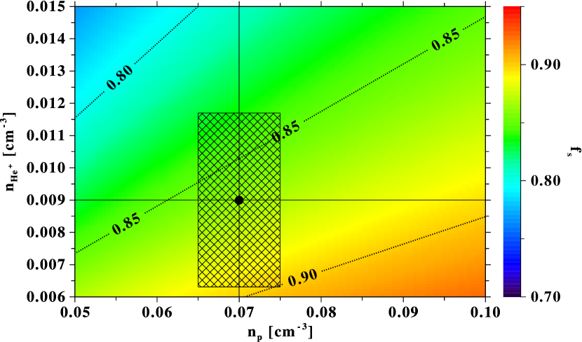
Figure 1: The multi-ion sound speed normalized to the proton sound speed as a function of the number densities $n_{p}$ and $n_{He^{+}}$. The black lines denote the ‘most likely values’ for the proton and $He^{+}$ number densities. The dotted lines are the contours for $f_{s}=0.8,0.85,0.9$

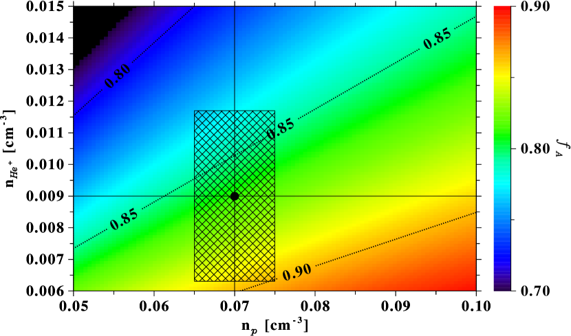
Figure 2: Same as Fig. 1, but for the Alfvén speeds.

In principle one has a five dimensional parameter space $(n_{p},n_{He^{+}},B,T,\vartheta)$. Here we will concentrate on the dependence of the speeds on $n_{He^{+}}$ and we will discuss the significance of the uncertainties in the other quantities in the next section.

In Fig. 1 the ratio $f_{s}=v_{s}/v_{s_{p}}$ of the multi-ion sound speed to the proton sound speed is plotted as a function of the number densities $n_{p}$ and $n_{He^{+}}$. Fig. 2 shows the correspding plot for the Alfvén speeds, i.e. $f_{A}=v_{A}/v_{A_{p}}$. The black lines indicate those speeds derived from the above most likely values, which are given together with magneto-sonic speeds in Table 1.

	protnons-only			proton+helium
$i$	$v_{i,p}$	$\pm\Delta v_{i,p}$	$\Delta v_{i,p}/v_{i,p}$	$v_{i}$	$\pm\Delta v_{i}$	$\Delta v_{i}/v_{i}$	$f_{i}=v_{i}/v_{p,i}$
	km/s	km/s	%	km/s	km/s	%
$s$	$9.35$	$0.22$	$0.022$	$8.07$	$0.64$	$0.079$	$0.86$
$A$	$24.73$	$4.20$	$0.17$	$20.10$	$4.02$	$0.20$	$0.81$
$fw(0^{o})$	$24.73$	$8.41$	$0.34$	$22.85$	$7.24$	$0.36$	$0.81$
$fw(45^{o})$	$25.30$	$8.37$	$0.33$	$20.62$	$7.12$	$0.35$	$0.82$
$fw(90^{o})$	$26.44$	$9.44$	$0.36$	$21.66$	$7.27$	$0.34$	$0.82$
$sw(0^{o})$	$9.35$	$0.033$	$3.7\cdot 10^{-4}$	$8.07$	$0.004$	$5.5\cdot 10^{-4}$	$0.86$
$sw(45^{o})$	$7.68$	$9.409$	$1.22$	$6.61$	$0.004$	$6.8\cdot 10^{-4}$	$0.86$
$sw(90^{o})$	$0.00$	$0.003^{*}$		$0.00$	$0.005^{*}$

Table 1: The most likely speeds and its errors for a proton-only and a proton-helium fluid. The last column gives the ratios between the proton-only to the proton-helium speeds $f_{i}=v_{i,p}/v_{i}$.

In Fig. 3 the fast magnetosonic wave speeds for the angles $\vartheta\in\{0^{o},45^{o},90^{o}\}$ are plotted. The red dot represent the values for the proton -only sound and Alfvén speeds given above, while the white dot determines the magnetosonic wave speed for the multi-ion speeds.

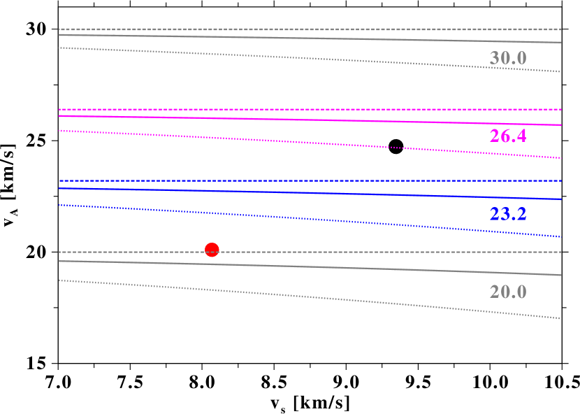
Figure 3: Fast magnetosonic speed (FMS) as function of $v_{s},v_{A}$ and $\vartheta$. The line types are the contours for the angles $\vartheta=0^{o}$ (dashed), $\vartheta=45^{o}$ (solid), and $\vartheta=90^{o}$ (dotted). The numbers give the corresponding FMSs. The black dot denotes the FMS for the ‘most likely values’ $v_{s_{p}},v_{A_{p}}$ for the protons-only, and the red dot is that for $v_{s},v_{A}$, i.e. including the $He^{+}$ contribution. The blue lines are the contours for a FMS of 23.2 $\mathrm{km/s}$, while the magenta lines that for 26.4 $\mathrm{km/s}$, which are identical with the respective LISM speeds as observed by IBEX (McComas et al., 2012b) and Ulysses (Witte, 2004). In the latter case the most likely value for the proton-only fluid lies below the solid line and thus the fluid is super-magnetosonic, while for the speed of 23.2$\mathrm{km/s}$ the lines always are below the black dot and thus the fluid is sub-magnetosonic. However, for the multi-fluid case, both LISM speeds are above the red dot, and hence the flow is super-fast magnetosonic. The gray lines give the values for FMS of 20 $\mathrm{km/s}$ and 30 $\mathrm{km/s}$, respectively.

From Fig. 3 we can deduce that for the most likely set of interstellar parameters the fast magnetosonic speed as well as the Alfvén and sound speeds are below the 23.2 km/s line and, thus, a bow shock must be expected to exist. In the following section we discuss in what range the error bars are.

5 Uncertainties of the characteristic speeds

The error $\Delta$ for a function $g(x_{1},...,x_{n})$ is given by:

$$\Delta g=\sqrt{\sum\limits_{i=1}^{n}\left(\Delta x_{i}\frac{\partial g(x_{1},...,x_{n})}{\partial x_{i}}\right)^{2}}$$ (7)

The relative errors $\Delta g/g$ for the sound speeds $v_{s_{p}}$ and $v_{s}$ yields:

$$\frac{\Delta v_{s_{p}}}{v_{s_{p}}} = \frac{\Delta T}{2T}$$ (8)

$$\frac{\Delta v_{s}}{v_{s}} = \sqrt{\left(\frac{\Delta T}{2T}\right)^{2}+\frac{9}{4\mu^{2}}\frac{\left(\frac{\Delta n_{p}}{n_{p}}\right)^{2}+\left(\frac{\Delta n_{He}}{n_{He^{+}}}\right)^{2}}{(1+\mu)^{2}(1+4\mu)^{2}}}$$

and, analogously, for the Alfvén speeds $v_{A_{p}}$ and $v_{A}$:

$$\frac{\Delta v_{A_{p}}}{v_{A_{p}}} = \sqrt{\left(\frac{\Delta B}{B}\right)^{2}+\left(\frac{\Delta n_{p}}{2n_{p}}\right)^{2}}$$ (9)

$$\frac{\Delta v_{A}}{v_{A}} = \sqrt{\left(\frac{\Delta B}{B}\right)^{2}+\frac{\left(\frac{\Delta n_{p}}{n_{p}}\right)^{2}+16\left(\frac{\Delta n_{He}}{n_{He^{+}}}\right)^{2}\mu^{2}}{4(1+4\mu)^{2}}}$$

The corresponding expressions for the magnetosonic speeds $v_{fw_{p},sw_{p}}$ and $v_{fw,sw}$ are very clumsy and were, therefore, calculated with the help of computer algebra system ‘wxmaxima’ and are not given here.

With the ‘most likely values’ as given above, i.e. $\Delta T/T=340/6300\approx 0.054$, $\Delta n_{p}/n_{p}=0.005/0.07\approx 0.07$, $\Delta n_{He^{+}}/n_{He^{+}}=0.009/0.015=0.02$, and $\Delta B/B=0.5/3=0.17$. we can calculate the relative uncertainties in the speeds $\Delta v_{i}/v_{i}$ ($i\in\{s,A,fw,fs\}$) for the sound, Alfvén, fast and slow magnetosonic speeds, given in Table 1 together with the extreme values $\vartheta=0^{o},90^{o}$. The reason for the large errors in the Alfvén speed is the uncertainty in the strength of the interstellar magnetic field, which determines those of the magnetosonic speeds. Obvioulsy, these uncertanities do not influence the main conclusion for the most likely values: The interstellar flow speed is likely to be super-fast magnetosonic and, thus, a fast bow shock must be expected to exist.

To complete the assessment, we would like to remark that if the ‘traditional’ value of 26.3 km/s for LISM inflow speed were correct, only magnetic field values above $>3.5\,\mu$G would remove the bow shock. Such rather extreme values of the magnetic field are discussed in Zieger et al. (2013) but are not favored by other authors (see, e.g., Zank et al., 2013).

6 Compression ratio of the bow shock

Given that it is likely that a fast bow shock exists it is interesting to estimate its strength. In ideal MHD the compression ratio $s$ at a shock fulfils the equation (Kabin, 2001):

$$0=(A_{1}^{2}-s)^{2}\left[A_{1}^{2}-\frac{2sS_{1}^{2}}{(s+1-\gamma(s-1))}\right]$$ (10)

$$-sk^{2}_{1}A_{1}^{2}\left[\frac{(2s-\gamma(s-1))}{(s+1-\gamma(s-1))}A_{1}^{2}-s\right]$$

with the abbreviations $A_{1}={M_{A_{1}}\cos\alpha}/{\cos(\alpha-\vartheta)}$, $S_{1}={M_{A_{1}}}/{M_{s_{1}}\cos(\alpha-\vartheta)}$, and $k_{1}=\tan{(\alpha-\vartheta)}$. Here $\alpha$ is the angle between the inflow direction and the shock normal, $\vartheta$ is the angle between the inflow and the magnetic field direction, and $M_{A_{1}},M_{s_{1}}$ are the Alfvénic and the sound wave Mach number upstream of the shock.

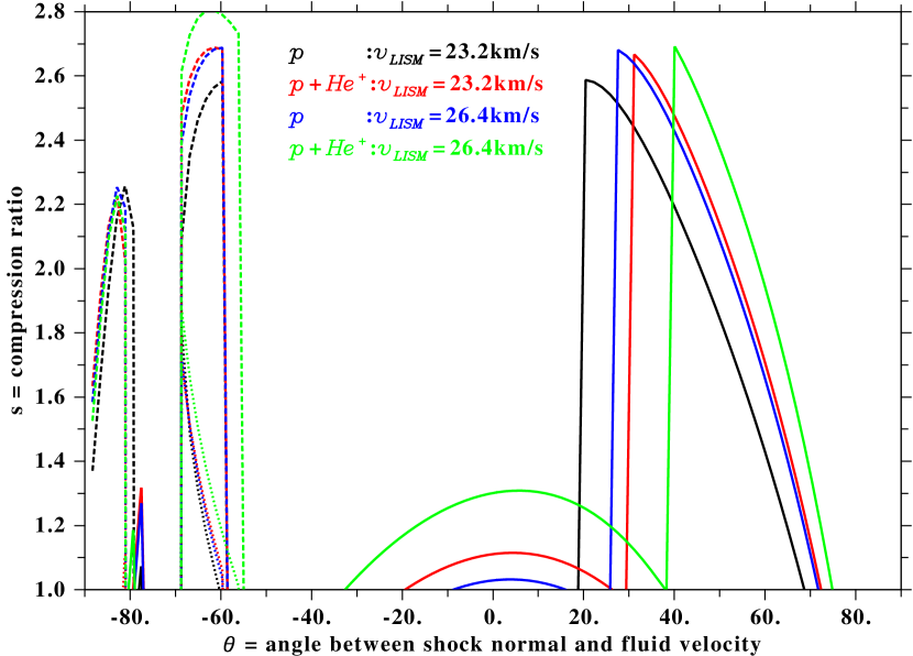
Figure 4: The compression ratio along the bow shock. The dashed and dotted lines denote the so-called intermediate shocks.

While a detailed analysis of the MHD shock structure – that should even be influenced by the presence of neutrals coupled via charge-exchange to the plasma (see, e.g., Lu et al., 2013) – would go far beyond the scope of this article, we nonetheless show with Fig. 4 that even an ideal MHD bow shock ahead of the heliopause has a complicated structure.

The figure gives a graphical representation of the solutions of equation 10, which can be reformulated as a cubic polynomial in the compression ratio $s$. The three groups of curves correspond to the three solutions and can be interpreted from left to right as intermediate, classical as well as slow shocks (Kabin, 2001). These solutions suggest that especially towards the flanks of the heliosphere the bow shock can be characterized as an intermediate rather than a classical one.

From the figure one expects that, most likely, a shock transition parallel to the inflow direction ($\alpha=0^{o}$) exists, at least, when the $He^{+}$ component in the interstellar medium is taken into account (Scherer et al., 2013).

Because an MHD shock structure can only be determined “a posteriori”, a detailed analysis of the MHD-shock behavior requires an MHD model including Helium. Such is not available at the moment, except that described by Izmodenov et al. (2003) and Malama et al. (2006) which are HD-models. Moreover, as was shown by Zank et al. (2013) energetic neutrals (ENAs) generated in the un-shocked solar wind can leak into the LISM and heat the latter. Because the charge exchange process does not change the number density of protons, the Alfvén speed $v_{A}$ is not affected, neither is the denominator in the sound speed given in Eq. 1. Only the nominator of the latter changes, and thus the sound speed will increase slightly (when we assume that the number density of ENAs and, hence, that of newly born ions is small compared to the interstellar proton density). As one can read off from Fig. 3 the dependence of the fast magnetosonic wave is weak as long as $v_{s}<v_{A}$. Hence, the overall conclusion remains: the bow shock is likely to exist.

7 Conclusion

We have demonstrated that the Alfvén and the fast magnetosonic wave speeds are – despite the uncertainties in the values characterizing the local interstellar medium – lower than the inflow speed of the interstellar medium and, thus, that a fast bow shock most likely exists. We arrived at this conclusion by explicitly taking into the account the effect of interstellar helium on the characteristic wave speeds. This result re-emphasises the need of including $He^{+}$ ions in the modeling of large-scale heliospheric structure.

We have also illustrated that the structure of the bow shock is more complicated than than that of a purely hydrodynamic one. In any case, the existence of the bow shock depends strongly on the strength of the local interstellar magnetic field, which will hopefully be measured in the near future by the Voyager 1 spacecraft that has recently crossed the heliopause (Gurnett et al., 2013).

References

- Barstow et al. (2005) Barstow, M. A., Cruddace, R. G., Kowalski, M. P., Bannister, N. P., Yentis, D., Lapington, J. S., Tandy, J. A., Hubeny, I., Schuh, S., Dreizler, S., & Barbee, T. W. 2005, MNRAS, 362, 1273
- Barstow et al. (1997) Barstow, M. A., Dobbie, P. D., Holberg, J. B., Hubeny, I., & Lanz, T. 1997, MNRAS, 286, 58
- Ben-Jaffel et al. (2013) Ben-Jaffel, J., Strumik, M., Ratkiewicz, R., & Grygorczuk, J. 2013, The Astrophysical Journal, 779, 130
- Boyd & Sanderson (2003) Boyd, T. J. M. & Sanderson, J. J. 2003, The Physics of Plasmas (Cambridge University Press)
- Bzowski et al. (2012) Bzowski, M., Kubiak, M. A., Möbius, E., Bochsler, P., Leonard, T., Heirtzler, D., Kucharek, H., Sokół, J. M., Hłond, M., Crew, G. B., Schwadron, N. A., Fuselier, S. A., & McComas, D. J. 2012, ApJS, 198, 12
- Bzowski et al. (2008) Bzowski, M., Möbius, E., Tarnopolski, S., Izmodenov, V., & Gloeckler, G. 2008, A&A, 491, 7
- Fahr et al. (1997) Fahr, H.-J., Fichtner, H., & Scherer, K. 1997, Space Sci. Rev., 79, 659
- Fahr & Ruciński (1999) Fahr, H. J. & Ruciński, D. 1999, A&A, 350, 1071
- Frisch et al. (2012) Frisch, P. C., Andersson, B.-G., Berdyugin, A., Piirola, V., DeMajistre, R., Funsten, H. O., Magalhaes, A. M., Seriacopi, D. B., McComas, D. J., Schwadron, N. A., Slavin, J. D., & Wiktorowicz, S. J. 2012, ApJ, 760, 106
- Gershman et al. (2013) Gershman, D. J., Gloeckler, G., Gilbert, J. A., Raines, J. M., Fisk, L. A., Solomon, S. C., Stone, E. C., & Zurbuchen, T. H. 2013, J. Geophys. Res., 118, 1389
- Gurnett et al. (2013) Gurnett, D. A., Kurth, W. S., Burlaga, L. F., & Ness, N. F. 2013, Science, 341, 1489
- Izmodenov et al. (2003) Izmodenov, V., Malama, Y. G., Gloeckler, G., & Geiss, J. 2003, ApJ, 594, L59
- Jenkins (2009) Jenkins, E. B. 2009, Space Sci. Rev., 143, 205
- Jenkins (2013) —. 2013, ApJ, 764, 25
- Kabin (2001) Kabin, K. 2001, Journal of Plasma Physics, 66, 259
- Lu et al. (2013) Lu, Q., Shan, L., Zhang, T., Zank, G. P., Yang, Z., Wu, M., Du, A., & Wang, S. 2013, ApJ, 773, L24
- Malama et al. (2006) Malama, Y. G., Izmodenov, V. V., & Chalov, S. V. 2006, A&A, 445, 693
- Marsch & Verscharen (2011) Marsch, E. & Verscharen, D. 2011, Journal of Plasma Physics, 77, 385
- McComas et al. (2012a) McComas, D. J., Alexashov, D., Bzowski, M., Fahr, H., Heerikhuisen, J., Izmodenov, V., Lee, M. A., Möbius, E., Pogorelov, N., Schwadron, N. A., & Zank, G. P. 2012a, Science, 336, 1291
- McComas et al. (2012b) McComas, D. J., Dayeh, M. A., Allegrini, F., Bzowski, M., DeMajistre, R., Fujiki, K., Funsten, H. O., Fuselier, S. A., Gruntman, M., Janzen, P. H., Kubiak, M. A., Kucharek, H., Livadiotis, G., Möbius, E., Reisenfeld, D. B., Reno, M., Schwadron, N. A., Sokół, J. M., & Tokumaru, M. 2012b, ApJS, 203, 1
- Möbius et al. (2012) Möbius, E., Bochsler, P., Bzowski, M., Heirtzler, D., Kubiak, M. A., Kucharek, H., Lee, M. A., Leonard, T., Schwadron, N. A., Wu, X., Fuselier, S. A., Crew, G., McComas, D. J., Petersen, L., Saul, L., Valovcin, D., Vanderspek, R., & Wurz, P. 2012, ApJS, 198, 11
- Scherer & Fahr (2003) Scherer, K. & Fahr, H. J. 2003, Annales Geophysicae, 21, 1303
- Scherer et al. (2013) Scherer, K., Fichtner, H., Fahr, H.-J., Bzowski, M., & Ferreira, S. 2013, A&A, ??, ??
- Slavin & Frisch (2008) Slavin, J. D. & Frisch, P. C. 2008, A&A, 491, 53
- Witte (2004) Witte, M. 2004, A&A, 426, 835
- Zank et al. (2013) Zank, G. P., Heerikhuisen, J., Wood, B. E., Pogorelov, N. V., Zirnstein, E., & McComas, D. J. 2013, ApJ, 763, 20
- Zieger et al. (2013) Zieger, B., Opher, M., Schwadron, N. A., McComas, D. J., & T th, G. 2013, GRL, n/a