Scanning-gate-induced effects in nonlinear transport through nanostructures

Abstract

We investigate the effect of a scanning gate tip on the nonlinear quantum transport properties of nanostructures. Generally, we predict that the symmetry of the current-voltage characteristic in reflection-symmetric samples is broken by a tip-induced rectifying conductance correction. Moreover, in the case of a quantum point contact (QPC), the tip-induced rectification term becomes dominant as compared to the change of the linear conductance at large tip-QPC distances. Calculations for a weak tip probing a QPC modeled by an abrupt constriction show that these effects are experimentally observable.

I Introduction

Nonlinear transport in semiconductor devices is the most common situation, but the analysis is considerably more complicated than in the linear case. While in the linear response regime a knowledge of the actual electric field distribution is not required to obtain the dissipation in the system, the field distribution does matter for many applications beyond linear transport.van Houten et al. (1992); Landauer (1987, 1989) Thus, a great difficulty facing nonlinear transport theories is the necessity to consider the self-consistent potential $\phi({\mathbf{r}})$ resulting from the imposed voltages between the probes and the electron-electron interactions in the device Büttiker (1993); Christen and Büttiker (1996) (i.e., the self-gating effect).

The use of a Scanning Tunneling Microscope (STM) to obtain information about the local field was proposed 25 years ago, Kirtley et al. (1988); Landauer (1989); van Houten et al. (1992) but only recently Jura et al. (2009, 2010); Kozikov et al. ; Brun et al. (2013) a related technique, the Scanning Gate Microscopy (SGM), has been applied in the nonlinear regime to study electron-electron scattering in a two-dimensional electron gas (2DEG) surrounding a Quantum Point Contact (QPC). The SGM appears as a less invasive probe than the STM, as it consists of a charged atomic force microscope scanning over the sample and thus modifying the conductance only through a capacitive coupling to the buried 2DEG.Binnig and Rohrer (1987); Giessibl (2003); Sellier et al. (2011)

The recent works of SGM in the nonlinear regime have been preceded by an important activity in the study of the tip-induced changes of the linear conductance through a QPC Topinka et al. (2000, 2001); LeRoy et al. (2005); Heller et al. (2005); Schnez et al. (2011) and other mesoscopic systems.Martins et al. (2007); Schnez et al. (2011); Kozikov et al. (2013) Even in the linear regime, the interpretation of the resulting scans is delicate.Jalabert et al. (2010); Gorini et al. (2013) On one hand, from various experimental and theoretical works focused on a QPC probed by a strongly charged tip, the conductance change appears to be closely related to the local current density.Topinka et al. (2001); LeRoy et al. (2005); Metalidis and Bruno (2005); Cresti (2006) On the other, it has been shown Gorini et al. (2013) that only under quite restrictive conditions (a spatially symmetric QPC tuned to a conductance plateau) the tip-induced conductance change is directly related to the current density at the tip position.

In the nonlinear regime the SGM of a QPC has delivered some intriguing results. The tip-induced conductance correction appears asymmetric in the bias voltage $V$ and reverses its sign for large $V$. Jura et al. (2010) While an interpretation in terms of the nonequilibrium distribution of electrons in a localized region of the 2DEG near the QPC was proposed, further experimental and theoretical work appeared necessary in order to justify the use of an effective electron temperature.Jura et al. (2010) Working in the regime of a partially closed QPC, an oscillatory splitting of the zero-bias anomaly with tip position, correlated with simultaneous appearances of the 0.7 anomaly, has been recently reported.Brun et al. (2013) These findings concerning an SGM setup in the regime of nonlinear transport through a QPC illustrate the need to address two related questions. Firstly, which is the local potential of a QPC operating in the nonlinear regime? van Houten et al. (1992); Martín-Moreno et al. (1992); Ouchterlony and Berggren (1995); Kristensen et al. (2000); Gloos et al. (2006); Song et al. (2009) Secondly, what is actually measured in the scanning gate microscopy of a QPC in the linear and nonlinear regimes?Jalabert et al. (2010); Sellier et al. (2011); Gorini et al. (2013); Schnez et al. (2011)

In this work we provide a theoretical approach to the SGM of a QPC operating in the nonlinear regime, by suitably generalizing the linear response approach of Refs. Jalabert et al., 2010; Gorini et al., 2013 within the general gauge-invariant framework defined in Ref. Christen and Büttiker, 1996. That is, in order to keep the problem tractable and to stay on a rigorous basis we limit ourselves to a gauge-invariant theory of weakly nonlinear transport, using a one-particle scattering approach and a perturbative tip. We underline the asymmetries appearing in nonlinear transport and predict two qualitative effects: (i) an odd-in-bias conductance correction induced by the tip in a nominally symmetric QPC; (ii) for increasing tip-QPC distances, a slower decay of the nonlinear conductance corrections as compared to the linear one. We investigate the quantitative behavior of the nonlinear conductance by solving the special case of an abrupt QPC subject to a finite bias. Recent experiments have shown that almost ideal, perfectly symmetric QPCs can be realized.Rössler et al. (2011) Tip-induced asymmetries should be observable in such systems and provide a signature of the probe’s invasiveness.

II Nonlinear transport coefficients

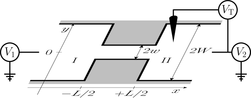
Figure 1: Sketch of the considered setup. A QPC in a two-dimensional electron gas is connected via wide leads to voltage sources generating voltages $V_{1}$ and $V_{2}$ in the left and right reservoir, respectively. An SGM tip acting in region II at the right of the constriction is at a voltage $V_{\mathrm{T}}$ with respect to $V_{2}$. For quantitative purposes, we use an abrupt geometry with a narrow region of width $2w$ and length $L$ between leads of width $2W$.

In the two-terminal configuration sketched in Fig. 1 the voltage $V_{1}$ ($V_{2}$) is imposed at the left (right) reservoir and the tip acting at the right of the QPC (region II) is at $V_{\mathrm{T}}$ with respect to $V_{2}$. While the depicted abrupt QPC is the example we use to calculate quantitative results, the general results that we will present are valid in any phase-coherent device. Gauge invariance implies that the measurable quantities do not change upon an overall shift of the energies of the problem. Thus, the current $I$ through the device does not depend on the reference voltage $U=(V_{1}+V_{2})/2$, but only on the bias voltage $V=V_{1}-V_{2}$ according to

$$I(V)=\frac{2e^{2}}{h}\left(g_{1}\ V+\frac{1}{2}\ g_{2}\ V^{2}+\frac{1}{3!}\ g_{3}\ V^{3}+\mathcal{O}(V^{4})\right)\,.$$ (1)

Scaling out the conductance quantum $2e^{2}/h$ allows us to work with the dimensionless differential conductance $g(V)=(h/2e^{2})\partial I/\partial V$, depending on the dimensionless linear, second-, and third-order conductances, $g_{1}$, $g_{2}$, and $g_{3}$, respectively. Within the general approach of Ref. Christen and Büttiker, 1996, for a two-terminal device operating at a low temperature $T$ (in the limit $k_{\mathrm{B}}T\ll\epsilon_{\mathrm{F}}$, with $k_{\mathrm{B}}$ the Boltzmann constant and $\epsilon_{\mathrm{F}}$ the Fermi energy) the key quantity describing electron transport is the screened transmission probability $\mathcal{T}(\varepsilon,\left\{V_{1},V_{2}\right\})=\mathrm{Tr}[t^{\dagger}t]$ depending on the energy $\varepsilon$ of the transmitted electron and on the applied voltages [through the self-consistent potential $\phi(\mathbf{r})$].

We use the standard notation of $t(t^{\prime})$ and $r(r^{\prime})$ for the transmission and reflection submatrices of the scattering matrix for particles impinging from the left (right) side of the scatterer and write

$$g_{1} = \mathcal{T}\,,$$ (2a)

$$g_{2} = (\partial_{V_{1}}-\partial_{V_{2}})\mathcal{T}=2\partial_{V}\mathcal{T}\,,$$ (2b)

$$g_{3} = (\partial_{V_{1}}\partial_{V_{1}}-\partial_{V_{1}}\partial_{V_{2}}+\partial_{V_{2}}\partial_{V_{2}})\mathcal{T}$$ (2c)

$$= [3\partial_{V}\partial_{V}+(1/4)\partial_{U}\partial_{U}]\mathcal{T}\,.$$

The second equalities follow from gauge invariance. The expressions involving $U$ and $V$-derivatives should be evaluated at ${(\epsilon_{\mathrm{F}},\left\{V=0,U=0\right\})}$, while the others at ${(\epsilon_{\mathrm{F}},\left\{V_{1}=V_{2}=0\right\})}$.

Figure 2: Unperturbed transmission probability $\mathcal{T}$ through an abrupt QPC with $L/w=2.5$ (see Fig. 1) as a function of the energy $\epsilon$. Solid, dashed, and dotted lines are evaluated from Eq. (15a) below for voltages $eV/\Delta_{1}=0$, $0.1$, and $0.2$, respectively, where $\Delta_{1}$ is the energy of the first quantized transverse mode in the constriction. The points “s” and “p” mark the positions in the step and on the plateau where Figs. 3 and 4 are evaluated, respectively. The inset shows the voltage dependence of the differential conductance, without tip, up to third order for different Fermi energies at the first step.

Starting without the SGM tip, we present in Fig. 2 the unperturbed transmission probability $\mathcal{T}$ as a function of $\epsilon$ for various bias voltages $V$, evaluated for the QPC sketched in Fig. 1. The unperturbed differential conductance up to third order $g^{(0)}=g^{(0)}_{1}+g^{(0)}_{2}V+(g^{(0)}_{3}/2)V^{2}$ is shown in the inset of Fig. 2. The $g_{i}^{(0)}$ are given by Eq. (2) when using as $\mathcal{T}$ the tip-unperturbed transition probability (to simplify the notation we do not write the index $(0)$ in $\mathcal{T}$ or in the scattering submatrices). The energy-dependent features in the transmission and conductance plateaus characteristic of clean abrupt geometries have been shown to be smoothed by finite temperature and bias.Szafer and Stone (1989); Lindelof and Aagesen (2008) The width of the conductance plateaus is considerably reduced only for rather large bias voltages Kouwenhoven et al. (1989) ($V\gtrsim\Delta_{1}/e$), where $\Delta_{1}$ is the lowest transverse energy in the constriction.

III Scanning-gate effects on transport coefficients

We now consider the action of an SGM tip. The voltage $V_{\mathrm{T}}$ is applied with respect to the reference $V_{2}$ in order to render the former gauge invariant. In an SGM setup the linear, second, and third-order conductances of the unperturbed device will change under the effect of a perturbing voltage $V_{\mathrm{T}}$. According to Ref. Jalabert et al., 2010, the tip-induced changes in the conductance coefficients $g_{i}^{(1)}$ are obtained when $\mathcal{T}$ in Eq. (2) is replaced by

$$\mu(\varepsilon,\left\{V_{1},V_{2}\right\}) = -4\pi\ \mathrm{Im}\left\{\mathrm{Tr}\left[r^{\dagger}t^{\prime}\ \mathcal{V}^{21}\right]\right\}$$ (3)

$$= -4\pi\ \mathrm{Im}\left\{\sum_{m=1}^{N}r_{m}^{*}t^{\prime}_{m}\mathcal{U}^{21}_{mm}\right\}\ .$$

The matrix elements of the perturbing potential $V_{\rm T}(\mathbf{r})$ in the basis of the scattering states $\Psi_{l,\varepsilon,a}$ are

$$\mathcal{V}^{\bar{l}l}_{\bar{a}a}=\int\mathrm{d}\mathbf{r}\ \Psi_{\bar{l},{\varepsilon},\bar{a}}^{*}(\mathbf{r})\ V_{\rm T}(\mathbf{r})\ \Psi_{l,\varepsilon,a}(\mathbf{r}),$$ (4)

where $l$ and $a$ represent the lead and mode, respectively, from which the scattering state (with energy $\varepsilon$) impinges. The scattering submatrices and the scattering states are those of the bias-dependent, tip-unperturbed problem. The last equality of Eq. (3) is obtained by a change into the basis of scattering eigenstates (built from the eigenmodes of $t^{\dagger}t$), Gorini et al. (2013) where the reflection and transmission submatrices are diagonal with non-zero elements $r_{m}$ ($r^{\prime}_{m}$) and $t_{m}$ ($t^{\prime}_{m}$) for $l=1,2$. $N$ is the number of channels in the leads and $\mathcal{U}^{21}_{m^{\prime}m}$ is the matrix element of the perturbing potential between the $m^{\prime}$^th left- and the $m$^th right-moving scattering eigenstates.

For a QPC $r_{m}t^{\prime}_{m}=0$ on a conductance plateau,Jalabert et al. (2010); Gorini et al. (2013) yielding a vanishing $\mu$. Moreover, away from the edges of the plateau the $V$ and $U$-derivatives of $r_{m}t^{\prime}_{m}$ also vanish, and thus $g_{i}^{(1)}=0$. Hence, the tip-induced changes in the linear, second, and third-order conductances are dominated by $g_{i}^{(2)}$. Those corrections scale as $V_{\mathrm{T}}^{2}$ and are obtained when $\mathcal{T}$ in Eq. (2) is replaced by

$$\nu(\varepsilon,\left\{V_{1},V_{2}\right\})=-4\pi^{2}\sum_{m,m^{\prime}=1}^{M}\mathcal{U}^{12}_{mm^{\prime}}\mathcal{U}^{21}_{m^{\prime}m},$$ (5)

where $M$ is the number of open channels in the constriction.

IV Tip-induced symmetry breaking

Various properties of the above discussed conductances, to different orders in $V$ and $V_{\mathrm{T}}$, can be studied depending on the characteristics of the QPC and the regime of operation. Interestingly, general properties can be inferred from symmetry considerations. Onsager’s relations for linear response Onsager (1931); Casimir (1945); Büttiker (1986) and their generalization to the nonlinear regime Löfgren et al. (2004); Sánchez and Büttiker (2004); Andreev and Glazman (2006) determine the symmetry of the response functions. For a left-right symmetric device in the absence of a magnetic field, the $I$-$V$ characteristics is odd, i.e. $I(-V)=-I(V)$ and $g_{2}^{(0)}=0$. This is the reason for the symmetry observed in the inset of Fig. 2. When a symmetric QPC is approached by a perturbing tip, the spatial symmetry is broken and one expects $g_{2}^{(1)}\neq 0$ at a conductance step and $g_{2}^{(2)}\neq 0$ on a conductance plateau. The tip-induced second-order conductance is a rectification effect, observable in nominally symmetric devices.

In order to quantify the above described effect one needs to solve the scattering problem with a finite bias, which requires modeling the constriction and the self-gating effect. The saddle-point model, applicable to smooth and relatively short QPCs, was the basis of numerous studies in the nonlinear regime,Martín-Moreno et al. (1992); Ouchterlony and Berggren (1995) and the close comparison with experiments allows to extract the constriction’s geometrical parameters.Gloos et al. (2006); Song et al. (2009) A symmetric potential drop between the reservoir and the bottleneck is compatible with experimental results.Martín-Moreno et al. (1992); Kristensen et al. (2000) The saddle-point model is appropriate for studies of the unperturbed conductance, determined by the features of the region immediately surrounding its narrowest point. However the tip-dependent conductance changes depend on the wave-functions far away from the bottleneck, where the saddle-point model does not provide a good description. This is why for an unbiased abrupt constriction, describing a hard-wall and relatively long QPC, a generalization of the mean-field approximation Szafer and Stone (1989) was developed to obtain the scattering eigenstates.Gorini et al. (2013)

In the biased case we assume the electric field to be non-zero only in the constriction itself. Such an assumption is supported by theoretical calculations showing that the potential drop for diffusive and ballistic constrictions occurs in the vicinity of the contact at distances of up to the order of the contact size,van Houten et al. (1992); Rokni and Levinson (1995) and has been used in numerical approaches yielding a reasonable account of weak nonlinear effects in abrupt QPCs.Castaño and Kirczenow (1990) Since we do not describe the physics of strong bias and half-plateaus,Glazman and Khaetskii (1989) but we only consider weak nonlinearities, assuming a linear potential drop between $V_{1}$ and $V_{2}$ within the constriction, without inelastic effects, is appropriate. In a symmetric QPC the potential drop does not have a quadratic component. Calculations up to $g_{3}$ are therefore consistent with our assumptions.

V Application to an abrupt quantum point contact

We consider an abrupt QPC (see Fig. 1) with hard wall boundaries confining the electrons to a narrow strip of length $L$ and width $2w$ in the central region, being directly attached to leads of width $2W$. The transverse channel wavefunctions are $\phi_{a}(y)=((-1)^{p}/\sqrt{W})\sin\left[q_{a}(y-W)\right]$, with $q_{a}=\pi a/2W$ and $p={\rm Int}\{a/2\}$. The outgoing $(+)$ and ingoing $(-)$ modes for left ($l=1$) and right ($l=2$) leads read

$$\varphi_{l\varepsilon a}^{(\pm)}(\mathbf{r})=\frac{c}{\sqrt{k_{la}}}\ e^{[\pm(-1)^{l}ik_{la}x]}\ \phi_{a}(y)\,,$$ (6)

with $\mathbf{r}=(x,y)$, $c=\sqrt{M_{\rm e}/2\pi\hbar^{2}}$, and longitudinal wavevectors satisfying $k_{la}^{2}=k_{l}^{2}-q_{a}^{2}$. Here $k_{l}=\sqrt{(2M_{\rm e}/\hbar^{2})(\varepsilon-eV_{l})}$, while $e$ and $M_{\rm e}$ stand for the charge and the effective mass of the electrons. The important difference with the linear case is that for a given energy $\varepsilon$ the longitudinal wave-vector $k_{la}$ differs at the two extremes of the junction according to the imposed voltages $V_{1}$ and $V_{2}$. Moreover, in the central region the scattering wave-function for electrons impinging from mode $a$ in lead $l$ is expanded as

$$\Psi_{l\varepsilon a}(\mathbf{r})=c\sum_{n=1}^{\infty}\left[\gamma^{+}_{lna}f_{n}(x)+\gamma^{-}_{lna}g_{n}(x)\right]\Phi_{n}(y)$$ (7)

with $\Phi_{n}(y)=(1/\sqrt{w})\sin\left[Q_{n}(y-w)\right]$ the transverse wavefunctions in the narrow region ($Q_{n}=n\pi/2w$), while $f_{n}(x)$ and $g_{n}(x)$ are the two Airy functions resulting from our assumption of a linear potential $\phi(\mathbf{r})$ within the constriction. The overlaps of the transverse channel wavefunctions

$$\mbox{\Fontauri A}_{na}=\int_{-w}^{w}\mathrm{d}y\,\Phi_{n}(y)\phi_{a}(y)\,,$$ (8)

together with the momentum-like quantity

$$\mathcal{K}_{lnn^{\prime}}={\sum_{a}}^{\prime}k_{la}\ \mbox{\Fontauri A}_{na}\mbox{\Fontauri A}_{n^{\prime}a}\,,$$ (9)

play a key role in the solution of the linear system of equations arising from the wave-function matching at $x=\pm L/2$.Gorini et al. (2013); Szafer and Stone (1989) (Here, ${\sum^{\prime}_{a}}$ denotes the sum over modes $a$ with the same parity as $n$ only). Since the $\mbox{\Fontauri A}_{na}$’s are appreciably different from zero only for $q_{a}\in[Q_{n-1},Q_{n+1}]$ and $k_{a}$ is a smooth function of $q_{a}$, one has $\mathcal{K}_{lnn^{\prime}}\approx\mathcal{K}_{ln}\delta_{nn^{\prime}}$. The above-cited approximations lead to the scattering amplitudes

$$t_{ba} = 2i{\mathcal{W}}\ \sqrt{k_{2b}k_{1a}}\ \exp{\left[-i\left(k_{2b}+k_{1a}\right)\frac{L}{2}\right]}\ \sum_{n}\frac{\mbox{\Fontauri A}_{nb}\mbox{\Fontauri A}_{na}}{\mathcal{D}_{n}}\,,$$ (10a)

$$r_{ba} = -\delta_{ba}\exp{[-ik_{1b}L]}+2i{\mathcal{W}}\ \sqrt{k_{1b}k_{1a}}\ \exp{\left[-i\left(k_{1b}+k_{1a}\right)\frac{L}{2}\right]}\ \sum_{n}\frac{\mathcal{B}_{1n}\mbox{\Fontauri A}_{nb}\mbox{\Fontauri A}_{na}}{\mathcal{D}_{n}}\ \,,$$ (10b)

$$t_{ba}^{\prime} = 2i{\mathcal{W}}\ \sqrt{k_{1b}k_{2a}}\ \exp{\left[-i\left(k_{1b}+k_{2a}\right)\frac{L}{2}\right]}\ \sum_{n}\frac{\mbox{\Fontauri A}_{nb}\mbox{\Fontauri A}_{na}}{\mathcal{D}_{n}}\,,$$ (10c)

$$r_{ba}^{\prime} = -\delta_{ba}\exp{[-ik_{2b}L]}+2i{\mathcal{W}}\ \sqrt{k_{2b}k_{2a}}\ \exp{\left[-i\left(k_{2b}+k_{2a}\right)\frac{L}{2}\right]}\ \sum_{n}\frac{\mathcal{B}_{2n}\mbox{\Fontauri A}_{nb}\mbox{\Fontauri A}_{na}}{\mathcal{D}_{n}}\ \,,$$ (10d)

with the definitions

$$\mathcal{D}_{n} = [\mathcal{L}^{+}_{1n}g_{n}(-L/2)][\mathcal{L}^{-}_{2n}f_{n}(L/2)]-[\mathcal{L}^{+}_{1n}f_{n}(-L/2)][\mathcal{L}^{-}_{2n}g_{n}(L/2)]\,,$$ (11a)

$$\mathcal{B}_{1(2)n} = g_{n}(\mp L/2)\mathcal{L}^{\mp}_{2(1)n}f_{n}(\pm L/2)-f_{n}(\mp L/2)\mathcal{L}^{\mp}_{2(1)n}g_{n}(\pm L/2)\,,$$ (11b)

where $\mathcal{L}^{\pm}_{ln}=\partial_{x}\pm i\mathcal{K}_{ln}$. The Wronskian of $f_{n}$ and $g_{n}$ is the constant ${\mathcal{W}}=-(1/\pi)[4\pi c^{2}eV/L]^{1/3}$ .

The solution (10) allows us to build the scattering eigenstates $\chi_{l\varepsilon m}$ as superposition of the scattering states $\Psi_{l\varepsilon a}$. The corresponding wave-function in the wide regions I and II, for a mode impinging from the left, can be asymptotically expressed as

$$\chi^{\mathrm{I}}_{1\varepsilon m}(\mathbf{r}) = \frac{c}{\sqrt{k_{1}}}\sqrt{\frac{2}{\pi\rho w}}\frac{\Theta_{m}^{\mathrm{I}}(\theta)}{\sqrt{\mathrm{Re}\{\mathcal{K}_{1m}\}}}\left\{e^{-i(k_{1}\rho-\pi/4)}+r_{m}e^{i(k_{1}\rho-\pi/4)}\right\}\,,$$ (12a)

$$\chi^{\mathrm{II}}_{1\epsilon m}(\mathbf{r}) = \frac{c}{\sqrt{k_{2}}}\sqrt{\frac{2}{\pi\rho w}}\frac{\Theta_{m}^{\mathrm{II}}(\theta)}{\sqrt{\mathrm{Re}\{\mathcal{K}_{2m}\}}}\ t_{m}e^{i(k_{2}\rho-\pi/4)}\,.$$ (12b)

For a mode impinging from the right, we have

$$\chi^{\mathrm{II}}_{2\varepsilon m}(\mathbf{r}) = \frac{c}{\sqrt{k_{2}}}\sqrt{\frac{2}{\pi\rho w}}\frac{\Theta_{m}^{\mathrm{II}}(\theta)}{\sqrt{\mathrm{Re}\{\mathcal{K}_{2m}\}}}\left\{e^{i(k_{2}\rho-\pi/4)}+r_{m}^{\prime}e^{-i(k_{2}\rho-\pi/4)}\right\}\,,$$ (13a)

$$\chi^{\mathrm{I}}_{2\epsilon m}(\mathbf{r}) = \frac{c}{\sqrt{k_{1}}}\sqrt{\frac{2}{\pi\rho w}}\frac{\Theta_{m}^{\mathrm{I}}(\theta)}{\sqrt{\mathrm{Re}\{\mathcal{K}_{1m}\}}}\ t_{m}^{\prime}e^{-i(k_{1}\rho-\pi/4)}\,.$$ (13b)

We denote $(\rho,\theta)$ the polar coordinates of $\mathbf{r}$ in a system centered at the entrance (exit) of the constriction when $\mathbf{r}$ is in region I (II). The angular dependence of the wavefunctions is given by

$$\Theta_{m}^{\mathrm{I}}(\theta) = (-1)^{m}\ \frac{Q_{m}k_{1}\cos\theta\,f_{m}(k_{1}w\sin\theta)}{(k_{1}\sin\theta)^{2}-Q_{m}^{2}}\,,$$ (14a)

$$\Theta_{m}^{\mathrm{II}}(\theta) = \frac{Q_{m}k_{2}\cos\theta\,f_{m}(k_{2}w\sin\theta)}{(k_{2}\sin\theta)^{2}-Q_{m}^{2}}\,,$$ (14b)

with $f_{m}(z)=-[e^{iz}-(-1)^{m}e^{-iz}]/2$. The transmission and reflection amplitudes associated with the scattering eignemodes are

$$t_{m} = t_{m}^{\prime}=2i\ \frac{\mathcal{W}}{\mathcal{D}_{m}}\sqrt{\mathrm{Re}\{\mathcal{K}_{1m}\}\ \mathrm{Re}\{\mathcal{K}_{2m}\}}\,$$ (15a)

$$r_{m} = \frac{2i\mathrm{Re}\{\mathcal{K}_{1m}\}\ \mathcal{B}_{1m}}{\mathcal{D}_{m}}-1\,,$$ (15b)

$$r_{m}^{\prime} = \frac{2i\mathrm{Re}\{\mathcal{K}_{2m}\}\ \mathcal{B}_{2m}}{\mathcal{D}_{m}}-1\,,$$ (15c)

From (15a) we get the transmission probability without the tip $\mathcal{T}$. Its energy dependence is shown in Fig. 2 for different values of the bias. From the expressions (12)-(13) of the scattering eigenstates, and given the tip potential $V_{\mathrm{T}}(\mathbf{r})$, we obtain the coefficients $\mu$, and $\nu$. We thus have closed expressions for the linear, second, and third-order conductances, as well as their tip-induced corrections. Fig. 3 presents the change of the differential conductance when an SGM tip scans the $x$-axis of an abrupt QPC tuned to the first conductance step (point “s” in Fig.2) for the case of a local tip potential $V_{\mathrm{T}}(\mathbf{r})=v_{\mathrm{T}}\delta(\mathbf{r}-\mathbf{r}_{\mathrm{T}})$.

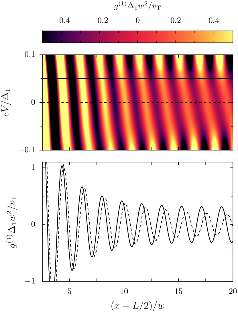
Figure 3: Upper panel: Colorscale plot of the tip-induced change of the differential conductance up to third-order terms, $g^{(1)}(V)=g_{1}^{(1)}+g_{2}^{(1)}V+g_{3}^{(1)}V^{2}/2$, as a function of bias voltage $V$ and tip position along the $x$-axis at the first conductance step ($\lambda_{\rm F}\approx 4w$, point “s” in Fig. 2) of the abrupt QPC sketched in Fig. 1 ($L/w=2.5$). The conductance correction is obtained to first order in a local tip potential. The tilt of the oscillating pattern in the upper panel at large tip-QPC distances is a signature of the tip-induced $V$-asymmetry. Lower panel: Dashed and solid lines correspond to the cuts indicated at $V=0$ and $eV=0.05\Delta_{1}$ in the upper panel.

We have chosen a symmetric device, where the vanishing of $g_{2}^{(0)}$ dictates that the differential conductance at low $V$ takes the form $g^{(0)}(V)=g_{1}^{(0)}+(g_{3}^{(0)}/2)V^{2}$. The $V$-symmetry observed in the inset of Fig. 2 is broken once a perturbing tip induces second-order corrections $g_{2}^{(1)}$. The “tilting” of the differential conductance pattern appearing in the top panel is an effect of the tip-caused breaking of the spatial and bias symmetries, and can be directly confronted with experiments. In the lower panel we present $g^{(1)}(V)$ (solid) and its linear contribution $g_{1}^{(1)}$ (dashed), corresponding to the indicated cuts at $V=0.05\Delta_{1}/e$ and $V=0$ in the upper panel, respectively.

The $\lambda_{\mathrm{F}}/2$-periodic oscillations characteristic of $g_{1}^{(1)}$ [Jalabert et al., 2010, Gorini et al., 2013] are also present in the nonlinear conductance corrections, with a phase shift building up at large distances. This phase shift could be related with the well-defined phase conditions observed as a function of $V$ in the difference of conductance changes between two tip positions.(Jura et al., 2009) Interestingly, while the oscillations decay as $(k_{\mathrm{F}}x)^{-1}$ for $g_{1}^{(1)}$, there is no such decay for the leading nonlinear term $g_{2}^{(1)}$, which dominates the conductance correction at large distances. The origin of this experimentally observable effect lies in the $V_{1(2)}$ dependence of the wave-vectors $k_{1(2)}$ and the $e^{2ik_{1(2)}x}$ terms present in the matrix elements of the tip-induced perturbation. Indeed, independently of the details of the model describing the system, if $g(\mathbf{r}_{T})$ shows interference fringes, then nonlinear corrections should become dominant away from the constriction. This observation is in line with recent experimental results, Brun et al. (2013); Brun and Sellier where the oscillating tip-induced corrections at finite bias voltage do not decrease in magnitude with increasing tip-QPC distances when scanning in some regions of the 2DEG adjacent to the QPC.

This is unusual, since an increase of $V$ has a radically different effect from that of a temperature rise. Starting from the linear regime, the temperature averaging effect would reduce the oscillations of $g_{1}^{(1)}$, while increasing $V$ leads to the dominance of $g_{2,3}^{(1)}$ with robust spatial oscillations.

Figure 4: The tip-induced change $g^{(2)}$ of the differential conductance up to third-order terms as in Fig. 3, but for the QPC tuned to the first conductance plateau (point “p” in Fig. 2), as a function of the tip position along the $x$-axis. Since $g^{(1)}$ is suppressed on plateaus, the lowest conductance correction is obtained to second order in the tip potential. The dashed and solid line corresponds to voltages of $V=0$ and $eV=0.1\Delta_{1}$, respectively. The dotted line shows the first rectifying nonlinear contribution $g_{2}^{(2)}V$ for the second voltage value.

The above-discussed rectification effect is the most prominent at conductance steps, and considerably reduced on a conductance plateau. The leading conductance corrections in the perturbative weak-probe limit for an abrupt QPC on the first conductance plateau are shown in Fig. 4. They are quadratic in $v_{\mathrm{T}}$ and dominated by the linear conductance correction $g_{1}^{(2)}$. The conductance corrections do not exhibit spatial oscillations, and the nonlinear rectifying contributions are relevant only for rather large values of $eV/\Delta_{1}$.

VI Conclusions

We have developed a gauge-invariant theory for the weak nonlinear effects of a nanostructure probed by Scanning Gate Microscopy. Despite working in the limit of a non-invasive probe, we have demonstrated that the tip can induce a nonlinear (rectifying) conductance in a geometrically symmetric device. We have quantified such an effect for the case of an abrupt QPC, showing it to be physically significant and experimentally attainable. At a conductance step the tip-generated lowest nonlinear transport coefficient $g_{2}$ shows $\lambda_{\mathrm{F}}/2$-periodic oscillations with an amplitude that does not decrease with the QPC-tip distance, as long as the transport remains phase-coherent. In particular, such a phenomenon should be model-independent and appear whenever the SGM signal shows such tip-position dependent oscillations.

The tip-induced oscillations between the 0.7 and the zero-bias anomalies observed in Ref. Brun et al., 2013 happen for bias voltages in the scale of $\mu V$. Subtle many-body effects are beyond the scope of the present work, based on a one-particle approach yielding results on the scale of the constriction quantization energy (${\rm m}eV$). Understanding the consequences that an SGM tip has on the differential conductance at such scales is a necessary ingredient in the interpretation of the experimental results.