Charge asymmetry in high-energy $\mu^{+}\mu^{-}$ photoproduction in the electric field of a heavy atom

Abstract

The charge asymmetry in the differential cross section of high-energy $\mu^{+}\mu^{-}$ photoproduction in the electric field of a heavy atom is obtained. This asymmetry arises due to the Coulomb corrections to the amplitude of the process (next-to-leading term with respect to the atomic field). The deviation of the nuclear electric field from the Coulomb field at small distances is crucially important for the charge asymmetry. Though the Coulomb corrections to the total cross section are negligibly small, the charge asymmetry is measurable for selected final states of $\mu^{+}$ and $\mu^{-}$. We further discuss the feasibility for experimental observation of this effect.

I Introduction

Photoproduction of muon pairs off heavy nuclei is one of the most interesting and important QED processes. The Born approximation cross section is known for arbitrary energy $\omega$ of the incoming photon, Refs. BH1934 ; Racah1934 (we set $\hbar=c=1$ throughout the paper). The Born cross section is proportional to the square of the nuclear form factor $F(Q^{2})$ and is sensitive to its shape since, for a heavy nucleus, the Compton wavelength of muon, $\lambda_{\mu}=1/m=1.87$ fm, is less than the nuclear radius, $R=7.3$ fm for gold and $R=7.2$ fm for lead, $m$ is the muon mass. Usually, for heavy atoms, one must account for the higher-order terms in the perturbative expansion with respect to the parameter $\eta=Z\alpha$ (Coulomb corrections), where $Z$ is the atomic charge number, $\alpha=e^{2}\approx 1/137$ is the fine-structure constant, and $e$ is the electron charge. The Coulomb corrections to the total cross section of muon pair photoproduction were discussed in a set of publications IM98 ; HKS07 ; JS09 . In contrast to the Born cross section, where the main contribution is given by the impact parameter $\rho$ in the region $R\ll\rho\ll\omega^{2}/m$, the main contribution to the Coulomb corrections stems from region $\rho\sim\lambda_{\mu}\lesssim R$. Thus, the Coulomb corrections to the total cross section are strongly suppressed by the form factor. Therefore, one may expect that this statement is also valid for all quantities related to the Coulomb corrections. In this paper we show that this is, in fact, not the case. We consider the charge asymmetry in the differential cross section $d\sigma(\bm{p},\,\bm{q},\,\eta)$ of high energy $\mu^{+}\mu^{-}$ photoproduction off a heavy atom, where $\bm{p}$ and $\bm{q}$ are the momenta of $\mu^{-}$ and $\mu^{+}$, respectively, $\omega\gg m$. The charge asymmetry $\cal A$ is defined as

$${\cal A}=\frac{d\sigma_{a}(\bm{p},\,\bm{q},\,\eta)}{d\sigma_{s}(\bm{p},\,\bm{q},\,\eta)}\,,\,d\sigma_{s}(\bm{p},\,\bm{q},\,\eta)=\frac{d\sigma(\bm{p},\,\bm{q},\,\eta)+d\sigma(\bm{q},\,\bm{p},\,\eta)}{2}\,,\,d\sigma_{a}(\bm{p},\,\bm{q},\,\eta)=\frac{d\sigma(\bm{p},\,\bm{q},\,\eta)-d\sigma(\bm{q},\,\bm{p},\,\eta)}{2}\,.$$ (1)

It follows from charge parity conservation that $d\sigma(\bm{p},\,\bm{q},\,\eta)=d\sigma(\bm{q},\,\bm{p},\,-\eta)\,,$ so that $d\sigma_{s}(\bm{p},\,\bm{q},\,\eta)$ is an even function of $\eta$ and $d\sigma_{a}(\bm{p},\,\bm{q},\,\eta)$ is an odd function of $\eta$. For $\omega\gg m$, small angles between the vectors $\bm{p}$ , $\bm{q}$, and incoming photon momentum $\bm{k}$, it is possible to make use of the quasiclassical approximation. The Coulomb corrections for the high energy $e^{+}e^{-}$ photoproduction cross section were obtained in the leading quasiclassical approximation in Refs.BM1954 ; DBM1954 . In this case the the nuclear form factor correction is negligible, and for a heavy nucleus the terms to all orders in the parameter $\eta$ should be taken into account. However, in the leading quasiclassical approximation $d\sigma_{a}(\bm{p},\,\bm{q},\,\eta)=0$, i.e., charge asymmetry is absent. The Coulomb corrections to the spectrum and to the total cross section of $e^{+}e^{-}$ photoproduction in a strong atomic field were derived in the next-to-leading quasiclassical approximation in Ref. LMS2004 . The Coulomb corrections to the differential cross section were derived in the next-to-leading quasiclassical approximation in Ref. LMS2012 , where the charge asymmetry $\cal A$ was studied in detail in all orders in $\eta$. For $\mu^{+}\mu^{-}$ high energy photoproduction, the structure of the Coulomb corrections to the differential cross section is different. When the momentum transfer $Q_{\perp}\gtrsim 1/R$ the form factor dependence strongly suppresses the cross section. Here $\bm{Q}=\bm{p}+\bm{q}-\bm{k}$, $\bm{Q}_{\perp}=\bm{Q}-(\bm{Q}\cdot\bm{\nu})\bm{\nu}$, and $\bm{\nu}=\bm{k}/\omega$. Therefore, to have the noticeable charge asymmetry and the noticeable cross section, we should consider the region $Q_{\perp}\lesssim 1/R$, but $p_{\perp}\sim q_{\perp}\sim m\gg Q_{\perp}$, so that $|\bm{p}_{\perp}+\bm{q}_{\perp}|\ll|\bm{p}_{\perp}-\bm{q}_{\perp}|$. As was shown in Ref. LMS2012 , in this region only the term $\propto\eta^{3}$ survives in the expansion of the Coulomb corrections in $\eta$ even for $\eta\sim 1$. In the present paper, we calculate $d\sigma_{a}(\bm{p},\,\bm{q},\,\eta)\propto\eta^{3}$ in the region $|\bm{p}_{\perp}+\bm{q}_{\perp}|\ll|\bm{p}_{\perp}-\bm{q}_{\perp}|$ taking into account the nuclear form factor correction. This term gives rise to the charge asymmetry $\cal A\propto\eta$. We show that $\cal A$ and $d\sigma_{s}(\bm{p},\,\bm{q},\,\eta)\propto\eta^{2}$ are large enough to be observed experimentally. The possibility of experimental observation of the charge asymmetry is discussed in detail. We also note that for $p_{\perp}\gg m$ , and $q_{\perp}\gg m$, $d\sigma_{a}$ was also investigated in Ref. BrGil68 in scalar electrodynamics.

II General discussion

The cross section for $\mu^{+}\mu^{-}$ pair production by a high-energy photon in an external field reads (see, e.g., Ref. BLP82 )

$$d\sigma=\frac{\alpha}{(2\pi)^{4}\omega}\,d\bm{p}_{\perp}\,d\bm{q}_{\perp}\,d\varepsilon_{p}\,|M_{\lambda_{1}\lambda_{2}\lambda_{3}}|^{2}\,,$$ (2)

where $\varepsilon_{p}=\sqrt{p^{2}+m^{2}}$, $\varepsilon_{q}+\varepsilon_{p}=\omega$, $\bm{p}$ and $\bm{q}$ are the $\mu^{-}$ and $\mu^{+}$ momenta, respectively, $\bm{p}_{\perp}$ and $\bm{q}_{\perp}$ are components of the vectors $\bm{p}$ and $\bm{q}$ perpendicular to the photon momentum $\bm{k}$ . The matrix element $M_{\lambda_{1}\lambda_{2}\lambda_{3}}$ has the form

$$M_{\lambda_{1}\lambda_{2}\lambda_{3}}\,=\,\int d\bm{r}\,\bar{u}_{\lambda_{1}\bm{p}}^{(out)}(\bm{r})\,\bm{\gamma}\cdot\bm{e}_{\lambda_{3}}\,v_{\lambda_{2}\bm{q}}^{(in)}(\bm{r})\exp{(i\bm{k}\cdot\bm{r})}\,\,.$$ (3)

Here $u_{\lambda_{1}\bm{p}}^{(out)}(\bm{r})$ is a positive-energy solution and $v_{\lambda_{2}\bm{q}}^{(in)}(\bm{r})$ is a negative-energy solution of the Dirac equation in the external field, $\lambda_{1}=\pm 1$ and $\lambda_{2}=\pm 1$ enumerate the independent solutions of the Dirac equation, and $\lambda_{3}=\pm 1$ enumerates the photon polarization vector, $\bm{e}_{\lambda_{3}}$, $\gamma^{\mu}$ are the Dirac matrices. Note that the asymptotic form of $u_{\lambda\bm{p}}^{(out)}(\bm{r})$ at large $\bm{r}$ contains the plane wave and the spherical convergent wave, while the asymptotic form of $v_{\lambda\bm{q}}^{(in)}(\bm{r})$ at large $\bm{r}$ contains the plane wave and the spherical divergent wave.

It is convenient to find the solutions of the Dirac equation in the atomic potential $V(r)$, using the relations (see , e.g., LMS2012 )

$$\frac{\exp(ipr_{2})}{4\pi r_{2}}\bar{u}_{\lambda{\bm{p}}}^{(out)}({\bm{r}}_{1})=-\lim_{r_{2}\to\infty}\,\frac{1}{2\varepsilon_{p}}\bar{u}_{\lambda{\bm{p}}}\gamma^{0}G({\bm{r}}_{2},{\bm{r}}_{1}|\varepsilon_{p})\,,\quad\bm{p}=p\bm{n}_{2}\,,$$

$$\frac{\exp(ipr_{1})}{4\pi r_{1}}v_{\lambda{\bm{p}}}^{(in)}({\bm{r}}_{2})=\lim_{r_{1}\to\infty}\,\frac{1}{2\varepsilon_{p}}G({\bm{r}}_{2},{\bm{r}}_{1}|-\varepsilon_{p})\gamma^{0}{v}_{\lambda{\bm{p}}}\,,\quad\bm{p}=p\bm{n}_{1}\,,$$

$$u_{\lambda{\bm{p}}}=\sqrt{\frac{\varepsilon_{p}+m}{2\varepsilon_{p}}}\begin{pmatrix}\phi_{\lambda}\\ \dfrac{{\boldsymbol{\sigma}}\cdot{\boldsymbol{p}}}{\varepsilon_{p}+m}\phi_{\lambda}\end{pmatrix}\,,\quad v_{\lambda{\bm{p}}}=\sqrt{\frac{\varepsilon_{p}+m}{2\varepsilon_{p}}}\begin{pmatrix}\dfrac{{\boldsymbol{\sigma}}\cdot{\boldsymbol{p}}}{\varepsilon_{p}+m}\chi_{\lambda}\\ \chi_{\lambda}\end{pmatrix}\,,$$ (4)

where $\bm{n}_{1}=\bm{r}_{1}/r_{1}$, $\bm{n}_{2}=\bm{r}_{2}/r_{2}$, and $G({\bm{r}}_{2},{\bm{r}}_{1}|\varepsilon)$ is the Green function of the Dirac equation in the atomic potential $V(r)$. We express the wave functions via the asymptotics of the Green function $D(\bm{r}_{2},\bm{r}_{1}|\,\varepsilon)$ of the squared Dirac equation,

$$D(\bm{r}_{2},\bm{r}_{1}|\varepsilon)=\langle\bm{r}_{2}|\left[(\varepsilon-V(r))^{2}-p^{2}-m^{2}+i\bm{\alpha}\cdot{\bm{\nabla}}V(r)+i0\right]^{-1}|\bm{r}_{1}\rangle\,,$$ (5)

where $\bm{\alpha}=\gamma^{0}\bm{\gamma}$. Using the relation

$$G(\bm{r}_{2},\bm{r}_{1}|\,\varepsilon)=\left[\gamma^{0}(\varepsilon-V(r_{2}))\,+i\bm{\gamma}\cdot\underrightarrow{{\bm{\nabla}}}_{2}\,+\,m\right]D(\bm{r}_{2},\bm{r}_{1}|\varepsilon)\,,$$

$$G(\bm{r}_{2},\bm{r}_{1}|\varepsilon)=D(\bm{r}_{2},\bm{r}_{1}|\,\varepsilon)\left[\gamma^{0}(\varepsilon-V(r_{1}))\,-i\bm{\gamma}\cdot\underleftarrow{{\bm{\nabla}}}_{1}\,+\,m\right]\,,$$ (6)

where $\underrightarrow{{\bm{\nabla}}}_{2}$ denotes the gradient over $\bm{r}_{2}$ acting to the right, while $\underleftarrow{{\bm{\nabla}}}_{1}$ denotes the gradient over $\bm{r}_{1}$ acting to the left. Using Eqs.(II) and (II), we arrive at the following result for the wave functions

$$\frac{\exp(ipr_{2})}{4\pi r_{2}}\bar{u}_{\lambda{\bm{p}}}^{(out)}({\bm{r}}_{2})=-\lim_{r_{2}\to\infty}\,\bar{u}_{\lambda{\bm{p}}}D({\bm{r}}_{2},{\bm{r}}_{1}|\varepsilon_{p})\,,\quad\bm{p}=p\bm{n}_{2},$$

$$\frac{\exp(ipr_{1})}{4\pi r_{1}}v_{\lambda{\bm{p}}}^{(in)}({\bm{r}}_{2})=-\lim_{r_{1}\to\infty}\,D({\bm{r}}_{2},{\bm{r}}_{1}|-\varepsilon_{p}){v}_{\lambda{\bm{p}}}\,,\quad\bm{p}=p\bm{n}_{1}\,.$$ (7)

It follows from Eqs. (5) and (II) that the wave functions $\bar{u}_{\lambda_{1}{\bm{p}}}^{(out)}({\bm{r}})$ and $v_{\lambda_{2}{\bm{q}}}^{(in)}({\bm{r}})$ have the form,

$$\bar{u}_{\lambda_{1}{\bm{p}}}^{(out)}({\bm{r}})=\bar{u}_{\lambda_{1}{\bm{p}}}\left[f_{0}(\bm{p},\bm{r})-\bm{\alpha}\cdot\bm{f}_{1}(\bm{p},\bm{r})-\bm{\Sigma}\cdot\bm{f}_{2}(\bm{p},\bm{r})\right]\,,$$

$$v_{\lambda_{2}{\bm{p}}}^{(in)}({\bm{r}})=\left[g_{0}(\bm{q},\bm{r})+\bm{\alpha}\cdot\bm{g}_{1}(\bm{q},\bm{r})+\bm{\Sigma}\cdot\bm{g}_{2}(\bm{q},\bm{r})\right]v_{\lambda_{2}{\bm{q}}}\,.$$ (8)

The term with $\gamma^{5}$ does not appear because it is impossible to construct a pseudoscalar using two vectors, $\bm{p}$ and $\bm{r}$. The functions $f_{0}(\bm{p},\bm{r})$, $\bm{f}_{1}(\bm{p},\bm{r})$, and $\bm{f}_{2}(\bm{p},\bm{r})$ may be obtained from the corresponding functions $g_{0}(\bm{q},\bm{r})$, $\bm{g}_{1}(\bm{q},\bm{r})$, and $\bm{g}_{2}(\bm{q},\bm{r})$ by the replacement $\bm{q}\rightarrow\bm{p}$ and $V(r)\rightarrow-V(r)$. Note that the perturbation expansion of the functions $f_{0}(\bm{p},\bm{r})$, $\bm{f}_{1}(\bm{p},\bm{r})$, and $\bm{f}_{2}(\bm{p},\bm{r})$ starts from the terms $V^{0}$, $V^{1}$ and $V^{2}$, respectively.

Let us introduce the quantities

$$(A_{00},\,\bm{A}_{01},\,\bm{A}_{10},\,\bm{A}_{02},\,\bm{A}_{20})=\int\!\!d\bm{r}\,\exp{(i\bm{k}\cdot\bm{r})}(f_{0}g_{0},\,f_{0}\bm{g}_{1},\,\bm{f}_{1}g_{0},\,f_{0}\bm{g}_{2}\,,\bm{f}_{2}g_{0})\,.$$ (9)

In terms of these quantities, we find

$$S = \frac{1}{2}\sum_{\lambda_{1},\lambda_{2},\lambda_{3}=\pm 1}|M_{\lambda_{1}\lambda_{2}\lambda_{3}}|^{2}=2(S_{0}+S_{1})\,,$$

$$S_{0} = \frac{1}{4}\left[\left(\frac{m\omega}{\varepsilon_{p}\varepsilon_{q}}\right)^{2}+\theta_{p}^{2}+\theta_{q}^{2}\right]|A_{00}|^{2}+|\bm{A}_{01}|^{2}+|\bm{A}_{10}|^{2}+\mbox{Re}\,A_{00}^{*}\left(\bm{\theta}_{p}\cdot\bm{A}_{10}+\bm{\theta}_{q}\cdot\bm{A}_{01}\right)\,,$$

$$S_{1} = -\mbox{Im}\,\left\{\left[\bm{A}_{20}^{*}\times\left(\bm{\theta}_{p}A_{00}+2\bm{A}_{10}\right)\right]\cdot\bm{\nu}+\left[\bm{A}_{02}^{*}\times\left(\bm{\theta}_{q}A_{00}+2\bm{A}_{01}\right)\right]\cdot\bm{\nu}\right\}\,,$$ (10)

where $\bm{\nu}=\bm{k}/\omega$, $\bm{\theta}_{p}=\bm{p}_{\perp}/\varepsilon_{p}$, $\bm{\theta}_{q}=\bm{q}_{\perp}/\varepsilon_{q}$. In deriving Eq.(II) we sum over the polarization of the $\mu^{+}$ and $\mu^{-}$ and average over the photon polarization. The expression for $S$ is very convenient for further consideration. It is obtained in the quasiclassical approximation with the first quasiclassical correction taken into account. Both terms, the leading term and the correction, are exact in the atomic field. For high energy $\mu^{+}\mu^{-}$ photoproduction, as it was discussed above, for the symmetric part of the cross section it is sufficient to use the Born result ($\propto V^{2}$), while for the antisymmetric part of the cross section we use the term $\propto V^{3}$. Note that the perturbation expansion of $A_{00}$, $\bm{A}_{10}$, and $\bm{A}_{01}$ starts from the terms $\propto V$, and the expansion of $\bm{A}_{20}$, and $\bm{A}_{02}$ starts from the terms $\propto V^{2}$.

III Calculation of the matrix elements and cross section

Figure 1: Diagrams of the perturbation theory for the wave function. The dashed line corresponds to the operator $2\varepsilon V(r)-i(\bm{\alpha}\cdot{\bm{\nabla}})V(r)$, and seagull corresponds to the operator $-V^{2}(r)$.

Using the conventional perturbation theory, see Eqs. (5), (II), and Fig.1, we find for the terms linear in the potential,

$$A_{00}^{(1)}=\frac{2\varepsilon_{p}\varepsilon_{q}V_{F}(Q^{2})}{\omega m^{2}}(\xi_{p}-\xi_{q})\,,\quad\bm{A}_{01}^{(1)}=-\frac{\varepsilon_{p}V_{F}(Q^{2})}{\omega m^{2}}\xi_{p}\bm{Q}\,,\quad\bm{A}_{10}^{(1)}=\frac{\varepsilon_{q}V_{F}(Q^{2})}{\omega m^{2}}\xi_{q}\bm{Q}\,,$$

$$\xi_{p}=\frac{1}{1+\delta_{p}^{2}}\,,\quad\xi_{q}=\frac{1}{1+\delta_{q}^{2}}\,,\quad\bm{\delta}_{p}=\frac{\varepsilon_{p}\bm{\theta}_{p}}{m}\,,\quad\bm{\delta}_{q}=\frac{\varepsilon_{q}\bm{\theta}_{q}}{m}\,,\quad\bm{Q}=\bm{p}+\bm{q}-\bm{k}\,.$$ (11)

Here $V_{F}(Q)$ is the Fourier transformation of the potential $V(r)$, $V_{F}(Q^{2})=-4\pi\eta{F}(Q^{2})/Q^{2}$, where ${F}(Q^{2})$ is the form factor which differs essentially from unity at $Q\gtrsim 1/R$ and $Q\lesssim 1/r_{scr}$, where $R$ is the nuclear radius and $r_{scr}$ is the screening radius. For $\mu^{+}\mu^{-}$ photoproduction, the effect of screening is negligible.

From Eqs.(II) and (III) we find the well known result for the leading term in $d\sigma_{s}$ (see, e.g.,BLP82 ):

$$d\sigma_{s}=\frac{2\alpha m^{2}\,d\varepsilon_{p}\,d\bm{\delta}_{p}\,d\bm{\delta}_{q}}{(2\pi)^{4}\omega^{3}}{V_{F}}^{2}(Q^{2})\left[\frac{Q^{2}}{m^{2}}\xi_{p}\xi_{q}(\varepsilon_{p}^{2}+\varepsilon_{q}^{2})+2\varepsilon_{p}\varepsilon_{q}(\xi_{p}-\xi_{q})^{2}\right]\,.$$ (12)

We now calculate the next-to-leading quasiclassical correction to the cross section. This correction is proportional to $V^{3}$ and arises from the interference between the leading term of the matrix element $\propto V$ and the next-to-leading term $\propto V^{2}$. Since $A_{00}^{(1)}$, $\bm{A}_{01}^{(1)}$, and $\bm{A}_{10}^{(1)}$ are the real quantities, one should calculate the real parts of $A_{00}^{(2)}$, $\bm{A}_{01}^{(2)}$, $\bm{A}_{10}^{(2)}$, and the imaginary parts of $\bm{A}_{02}^{(2)}$ and $\bm{A}_{20}^{(2)}$, see Eq. (II). A straightforward calculation gives

$$\mbox{Re}A_{00}^{(2)}=\frac{\varepsilon_{p}\xi_{p}+\varepsilon_{q}\xi_{q}}{\omega m^{2}}(J_{0}-J_{1})\,,$$

$$\mbox{Re}\bm{A}_{01}^{(2)}=\frac{\varepsilon_{p}\xi_{p}}{2\varepsilon_{q}\omega m^{2}}J_{1}\bm{Q}\,,\quad\mbox{Re}\bm{A}_{10}^{(2)}=\frac{\varepsilon_{q}\xi_{q}}{2\varepsilon_{p}\omega m^{2}}J_{1}\bm{Q}\,,$$

$$\mbox{Im}\bm{A}_{02}^{(2)}=\frac{\varepsilon_{p}\xi_{p}}{2\varepsilon_{q}\omega m^{2}}J_{0}[\bm{\nu}\times\bm{Q}]\,,\quad\mbox{Im}\bm{A}_{20}^{(2)}=\frac{\varepsilon_{q}\xi_{q}}{2\varepsilon_{p}\omega m^{2}}J_{0}[\bm{\nu}\times\bm{Q}]\,,$$

$$J_{0}=\int\frac{d\bm{s}}{(2\pi)^{3}}V_{F}(\chi_{+})V_{F}(\chi_{-})\,,\quad J_{1}=\int\frac{d\bm{s}}{(2\pi)^{3}}(4s_{\parallel}^{2}-Q^{2})V_{F}(\chi_{+})V_{F}^{\prime}(\chi_{-})\,,$$

$$\chi_{\pm}=(\bm{s}\pm\bm{Q}/2)^{2}\,,\quad s_{\parallel}=\bm{s}\cdot\bm{Q}/Q$$ (13)

where $V_{F}^{\prime}(\chi)=\partial V_{F}(\chi)/\partial\chi$. Using Eqs.(III), (III) and (II), we obtain the antisymmetric part of the cross section,

$$d\sigma_{a} = \,\frac{\alpha m^{2}d\varepsilon_{p}\,d\bm{\delta}_{p}\,d\bm{\delta}_{q}}{(2\pi)^{4}\omega^{3}}\,\bigg{\{}(\xi_{p}-\xi_{q})\bigg{[}4(\varepsilon_{p}\xi_{p}+\varepsilon_{q}\xi_{q})+\frac{\omega(\varepsilon_{p}^{2}+\varepsilon_{q}^{2})}{\varepsilon_{p}\varepsilon_{q}}\bigg{]}$$ (14)

$$+(\varepsilon_{p}-\varepsilon_{q})\frac{(\varepsilon_{p}^{2}+\varepsilon_{q}^{2})}{\varepsilon_{p}\varepsilon_{q}}\,\frac{Q^{2}}{m^{2}}\xi_{p}\xi_{q}\bigg{\}}V_{F}(Q^{2})(J_{0}-J_{1})\,.$$

For the Coulomb field, the calculation yields $J_{0}=2\pi^{2}\eta^{2}/Q$, and $J_{1}=0$. Thus, our result is in agreement with the result obtained in Ref. LMS2012 . In the formula for the charge asymmetry, ${\cal A}=d\sigma_{a}/d\sigma_{s}$, the dependence on the nuclear radius enters via the ratio $(J_{0}-J_{1})/V_{F}(Q^{2})$. Very often the form factor is approximated by the formula $F_{0}(Q^{2})=1/(1+Q^{2}/\Lambda^{2})$, where $\Lambda\approx 80$ MeV for heavy nuclei. This approximation gives an accurate result up to $60$ MeV. In this case the function ${\cal F}(Q)=-2(J_{0}-J_{1})/(\pi\eta QV_{F}(Q^{2}))$ has the simple form

$${\cal F}(Q) = (1+x^{2})\left[1+\frac{2}{\pi}\arcsin\left(\frac{x}{\sqrt{x^{2}+4}}\right)-\frac{4}{\pi}\arcsin\left(\frac{x}{\sqrt{x^{2}+1}}\right)\right]-\frac{12x}{\pi(4+x^{2})}\,,\quad x=\dfrac{Q}{\Lambda}\,.$$ (15)

At $Q\ll\Lambda$, we have ${\cal F}(Q)\approx 1-\displaystyle{\frac{6Q}{\pi\Lambda}}$, so that the function ${\cal F}(Q)$ diminishes rapidly with increasing $Q$. In Fig.2 we show the dependence of the function ${\cal F}(Q)$ on $Q$ for lead ($Z=82$). The solid curve corresponds to the real charge distribution, while the dashed curve is given by Eq.(15) with $\Lambda=60$ MeV.

Figure 2: The dependence of the function ${\cal F}(Q)$ on $Q$ for lead ( $Z=82$). The solid curve corresponds to the real charge distribution, the dashed curve is given by Eq.(15) with $\Lambda=60$ MeV.

For $Q\ll|\bm{p}_{\perp}-\bm{q}_{\perp}|$, the formula (14) simplifies to,

$$d\sigma_{a}=\,\frac{\alpha m^{2}d\varepsilon_{p}\,d\bm{\delta}_{p}\,d\bm{\delta}_{q}}{(2\pi)^{4}\omega^{2}}\,(\xi_{p}-\xi_{q})\bigg{[}2(\xi_{p}+\xi_{q})+\frac{(\varepsilon_{p}^{2}+\varepsilon_{q}^{2})}{\varepsilon_{p}\varepsilon_{q}}\bigg{]}V_{F}(Q^{2})(J_{0}-J_{1})\,.$$ (16)

And we obtain for the charge asymmetry

$${\cal A}=\,\frac{\pi\eta m\omega\kappa(\xi_{p}+\xi_{q}+B)}{4\varepsilon_{p}\varepsilon_{q}(B+\kappa^{2}\xi_{p}\xi_{q})}{\cal F}(Q)\,,$$

$$B=\frac{\varepsilon_{p}^{2}+\varepsilon_{q}^{2}}{2\varepsilon_{p}\varepsilon_{q}}\,,\quad\kappa=\frac{m(\xi_{q}-\xi_{p})}{Q\xi_{p}\xi_{q}}\,,$$ (17)

Let $\chi$ is the angle between the vectors $\bm{p}_{\perp}$ and $-\bm{q}_{\perp}$. In order to estimate $\cal A$, let us consider the region of interest from the experimental point of view, $|\chi|\ll|\varepsilon_{p}-\varepsilon_{q}|/\omega\ll 1$ and $|\theta_{p}-\theta_{q}|/|\theta_{p}+\theta_{q}|\ll|\varepsilon_{p}-\varepsilon_{q}|/\omega$. In this region,

$${\cal A}=\,\frac{\pi\eta\theta(1+2\xi)}{(1+4\xi^{2}\delta^{2})}{\cal F}(\theta|\varepsilon_{p}-\varepsilon_{q}|)\,\mbox{sgn}(\varepsilon_{p}-\varepsilon_{q})\,,$$

$$\theta=\frac{1}{2}(\theta_{p}+\theta_{q}),\quad\delta=\frac{\omega\theta}{2m},\quad\xi=\frac{1}{1+\delta^{2}}\,,$$ (18)

and all of the dependence on $\varepsilon_{p}-\varepsilon_{q}$ is contained in the function $\cal F$. Since Eq. (III) is valid for all $\eta\lesssim 1$, the prefactor of $\cal F$ in Eq. (III) can easily reach ten percent or more.

IV Possibility of experimental observation

The above calculations clearly show that the size of the asymmetry is within reach of current experimental capabilities, suggesting a possible measurement. Due to the low cross section, however, no current photon facility has the required photon beam flux for such a measurement. We thus propose to make use of an electron beam to provide the (virtual) photon flux, where we may calculate the equivalent photon flux close to the end-of-spectrum using the approximation, see, e.g., Ref. BFKK81 :

$$N_{\gamma}=\frac{\alpha}{\pi}\frac{\Delta}{E}\ln\left(\frac{\Delta}{m_{e}}\right)N_{e},$$ (19)

where $N_{\gamma}$($N_{e}$) is the photon (electron) flux, $E$ is the electron beam energy, $m_{e}$ is the electron mass, and $\Delta$ is the region of integration around the endpoint. Eq. (19) is valid for $m_{e}\ll\Delta\ll E$. We identify two facilities with experimental capabilities suitable for the proposed measurement. Those are the experimental Hall A at the Thomas Jefferson National Accelerator Facility Alcorn:2004sb , and the A1 experimental hall at the Mainzer Mikrotron Blomqvist:1998xn . We work in a region where the muon angles are equal, $\theta_{\mu}^{+}=\theta_{\mu}^{-}$, and the the sum of the muon energies is close to the beam energy, $E_{\mu}^{+}+E_{\mu}^{-}\sim E$, so that the momentum transfer to the recoiling nucleus is minimal, making the asymmetry essentially independent of the nuclear form factor. The proposed kinematic conditions for both facilities are summarized in Table 1.

	JLab	Mainz
Beam Energy	2.2 GeV	1.5 GeV
Current	50 $\mu$A	50 $\mu$A
Detector Package	HRS + Septa magnets (see text)	Dedicated (see text)
Detector Angle	$5^{\circ}$	$5^{\circ}$
Target	238U (25 $\mu$m)	238U (25 $\mu$m)

Table 1: Proposed kinematical conditions.

We assume a conservative solid angle of 0.3 msr for each of the detectors, an energy bin of 10 MeV, and select events where the sum of the muon energies is within 10 MeV of the beam energy,

$$E-(E_{\mu^{+}}+E_{\mu^{-}})\leq 10{\rm MeV}.$$ (20)

Figure 3 shows the calculated asymmetry and projected asymmetry as a function of $\delta=E_{\mu^{+}}-E_{\mu^{-}}$ for the aforementioned kinematics, where we assume 3h of beam time for each of the data points.

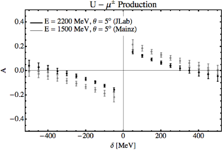
Figure 3: Calculated asymmetries and projected uncertainties for the experimental conditions described in the text.

The proposed JLab experimental setup is essentially identical (except for the target) to the already approved JLab experiment E12-10-009 (APEX) APEX , searching for massive vector bosons (dark photons) Bjorken:2009mm . Thus, the proposed measurement can be trivially conducted jointly with the APEX experiment. The MAMI/A1 detector setup is currently unsuitable for the proposed experiment, due to the constraints on the possible detector angles, thus, a dedicated detector setup would be required. Due to the relaxed requirement on the particle detection (muons with energies between about 500 MeV and 1 GeV and a small solid angle) such a detector setup is relatively easy to construct or obtain, as an example we mention the di-electron production experiment, currently scheduled at the HIGS facility, which makes use of an appropriate detector setup and which is expected to conclude data taking during 2014 or 2015. Fig. 3 clearly demonstrates the viability of such an experiment, which will be the first to accurately measure di-muon production off heavy nuclei, where the parameter $\eta$ is not small. Also note that in these experimental conditions it is possible to observe a second sign reversal of the asymmetry, which happens due to cancellation in the function ${\cal F}(Q)$ (see Fig. 2)

V Conclusion

We have derived the charge asymmetry ${\cal A}$ in the process of $\mu^{+}\mu^{-}$ photoproduction in the electric field of a heavy atom. This asymmetry is related to the first quasiclassical correction to the differential cross section of the process. In the experimental region of interest, where $Q\ll|\bm{p}_{\perp}-\bm{q}_{\perp}|$, $Q\sim 1/R$, and $p_{\perp}\sim q_{\perp}\sim 1/m$, the asymmetry ${\cal A}$ can be as large as a few tens of percent. In this region our result is valid even for $\eta\sim 1$. Since $\lambda_{\mu}\lesssim R$, the charge asymmetry is very sensitive to the shape of the nuclear form factor and may be used to validate or perform measurements of these form factors. Additionally, measurements of ${\cal A}$ can be used to investigate not only the nuclear form factor, but also to search for new massive particles such as dark photons Bjorken:2009mm , and by comparing results from electron and muon production, test lepton universality. Finally, we have demonstrated that the experimental observation of the charge asymmetry in $\mu^{+}\mu^{-}$ photoproduction in the electric field of heavy atoms is a realistic task and suggested an experimental configuration which will allow such a measurement.

References

• (1) H.Β A. Bethe and W.Β Heitler, Proc. R. Soc. London A146, 83 (1934).
• (2) G.Β Racah, Nuovo Cim. 11, 461 (1934).
• (3) D. Ivanov, K. Melnikov, Phys. Rev. D 57, 4025 (1998).
• (4) K. Hencken, E. A. Kuraev, V. G. Serbo, Phys. Rev. C, 75, 034903 (2007).
• (5) U. D. Jentschura, V. G. Serbo, Eur. Phys. J. C, 64, 309 (2009).
• (6) H.Β A. Bethe and L.Β C. Maximon, Phys. Rev. 93, 768 (1954).
• (7) H.Β Davies, H.Β A. Bethe, and L.Β C. Maximon, Phys. Rev. 93, 788 (1954).
• (8) R.Β N. Lee, A.Β I. Milstein, and V.Β M. Strakhovenko, Phys. Rev. A 69, 022708 (2004).
• (9) R.Β N. Lee, A.Β I. Milstein, and V.Β M. Strakhovenko, Phys. Rev. A 85, 042104 (2012).
• (10) S.J. Brodsky and J.R. Gillespie, Phys. Rev. 173, 1011 (1968).
• (11) V.Β B.Berestetski, E.Β M.Lifshits, L.Β P.Pitayevsky, Quantum electrodynamics (Pergamon, Oxford, 1982).
• (12) A.I. Milstein, I.S. Terekhov, Zh. Eksp. Teor. Fiz. 125, 785 (2004) [JETP 98, 687 (2004)].
• (13) V.N. Baier, V.S. Fadin, V.A. Khoze, and E.A. Kuraev, Physics Reports 78, 293 (1981).
• (14) J.Β Alcorn, B.Β D.Β Anderson, K.Β A.Β Aniol, J.Β R.Β M.Β Annand, L.Β Auerbach, J.Β Arrington, T.Β Averett and F.Β T.Β Baker et al., Nucl.Β Instrum.Β Meth.Β A 522, 294 (2004).
• (15) K.Β I.Β Blomqvist, W.Β U.Β Boeglin, R.Β Bohm, M.Β Distler, R.Β Edelhoff, J.Β Friedrich, R.Β Geiges and P.Β Jennewein et al., Nucl.Β Instrum.Β Meth.Β A 403, 263 (1998).
• (16) Jefferson Lab Experiment E12-10-009, http://hallaweb.jlab.org/experiment/APEX/
• (17) J.Β D.Β Bjorken, R.Β Essig, P.Β Schuster and N.Β Toro, Phys.Β Rev.Β D 80, 075018 (2009) [arXiv:0906.0580 [hep-ph]].