The BICEP2 data and a single Higgs-like interacting tachyonic field

Abstract

It is proposed that the recently announced BICEP2 value of tensor-to scalar ratio $r\sim 0.2$ can be explained as containing an extra contribution from the recent acceleration of the universe. In fact this contribution, being robust, recent and of much longer duration (by a large order of magnitude) may dominate the contribution from the inflationary origin. In a possible scenario, matter (dark or baryonic) and radiation etc. can emerge from a single Higgs-like tachyonic scalar field in the universe through a physical mechanism not yet fully known to us. The components interact among themselves to achieve the thermodynamical equilibrium in the evolution of the universe. The field potential for the present acceleration of the universe would give a boost to the amplitude of the tensor fluctuations of gravity waves generated by the early inflation and the net effects may be higher than the earlier PLANCK bounds. In the process, the dark energy, as a cosmological constant decays into creation of dark matter. The diagnostics for the three-component, spatially homogeneous tachyonic scalar field are discussed in detail. The components of the field with perturbed equation of state are taken to interact mutually and the conservation of energy for individual components gets violated. We study mainly the $O_{m}(x)$ diagnostics with the observed set of $H(z)$ values at various redshifts, and the dimensionless state-finders for these interacting components. This analysis provides a strong case for the interacting dark energy in our model.

I Introduction

The recent announcement of BICEP2 observations a0 of the tensor-to-scalar ratio $r\sim 0.20$ claim the B-mode polarisation signatures to be produced completely due to the primordial gravity waves arising from the early inflation. However, we think that this belief is misplaced and the observed value of $r$ must include the contributions not only from the early inflation but also the contributions from the present acceleration of the universe. In fact, this acceleration being of the recent origin and of a much longer duration (by many orders) must contribute significantly, and so the later contributions on the B-mode polarisation of the Cosmic Microwave Background Radiation (CMBR) must be more marked than due to the early inflation, whose sole contribution was reported by Planck a00 .

We recall that the cosmological and astrophysical observations support the fact our universe is in accelerated expansion phase a1 ; a2 ; a3 , albeit the exact form of scale factor has not yet been fixed by any observations. Heading from this motivation previously we adopted the quasi-exponential expansion that can also produce the significant tensor fluctuations of spacetime a4 . In q2 the cosmological constant $\Lambda$ with the energy density of the self-interaction of scalar bosons bound in a condensate is identified. In this approach, $\Lambda$ decay provides with a dynamical realization of spontaneous symmetry breaking. The detailed kinematics of $\Lambda$ decay and the back reaction of the decay products on the $\Lambda$ dynamics are given in q3 . The slow evaporation regime is found here for a wide range of possible parameters of particle interactions.

The present paper is organised into five sections. In section $(2)$ we study the mutual interaction among the Higgs-like tachyon field components wherein the gravity waves unleashed by the earlier inflation may be further boosted by the present acceleration of the universe, and may appear beyond the PLANCK upper bounds a00 . Section $(3)$ is laid for $O_{m}(x)$-diagnostic and section $(4)$ is devoted towards $O_{m}3(x)$-diagnostic and statefinder parameters for interacting components of tachyonic field. The Lagrangian for the tachyonic scalar field appears from string theory n1 and is given from the action

$$\mathcal{A}=\int d^{4}x\sqrt{-g}\left(\frac{R}{16\pi G}-V(\phi)\sqrt{1-\partial^{i}\phi\partial_{i}\phi}\right)$$ (1)

as

$$\mathcal{L}=-V(\phi)\sqrt{1-\partial^{i}\phi\partial_{i}\phi}$$ (2)

whereas the energy-momentum tensor

$$T^{ik}=\frac{\partial\mathcal{L}}{\partial(\partial_{i}\phi)}\partial^{k}\phi-g^{ik}\mathcal{L}$$ (3)

leads to pressure and energy density of the tachyonic scalar field as

$$P=-V(\phi)\sqrt{1-\partial^{i}\phi\partial_{i}\phi}$$ (4)

and

$$\rho=\frac{V(\phi)}{\sqrt{1-\partial^{i}\phi\partial_{i}\phi}}.$$ (5)

For spatially homogeneous tachyonic scalar field we have

$$P=-V(\phi)\sqrt{1-\dot{\phi}^{2}}$$ (6)

$$\rho=\frac{V(\phi)}{\sqrt{1-\dot{\phi}^{2}}}.$$ (7)

Here, we assume that radiation with equation of state

$$w_{r}=1/3$$

also exists as one inherent component of same tachyonic scalar field. Due to some physical mechanism not known in detail at present to us, but that may be like a Higgs mechanism, we can split the expressions (6) and (7) as

$$P=-\frac{V(\phi)}{\sqrt{1-\dot{\phi}^{2}}}+\frac{\dot{\phi}^{2}V(\phi)}{\sqrt{1-\dot{\phi}^{2}}}+0$$ (8)

$$\rho=\frac{V(\phi)}{\sqrt{1-\dot{\phi}^{2}}}+\frac{3\dot{\phi}^{2}V(\phi)}{\sqrt{1-\dot{\phi}^{2}}}-\frac{3\dot{\phi}^{2}V(\phi)}{\sqrt{1-\dot{\phi}^{2}}}.$$ (9)

From (8) and (9) it is seen that when we include radiation in tachyonic scalar field then one new exotic component also appears (say, exotic matter since its energy density is negative) with zero pressure. Thus, the tachyonic scalar field resolves into three components say $a$, $b$ and $c$. The pressure and energy density of $a$ is given as

$$P_{a}=-\frac{V(\phi)}{\sqrt{1-\dot{\phi}^{2}}},\quad\rho_{a}=\frac{V(\phi)}{\sqrt{1-\dot{\phi}^{2}}}\Rightarrow w_{a}=-1=w_{\lambda}.$$

This is nothing but the ‘true’ cosmological constant because of its equation of state being $w_{\lambda}=-1$.

The second component with

$$P_{b}=\frac{\dot{\phi}^{2}V(\phi)}{\sqrt{1-\dot{\phi}^{2}}},\quad\rho_{b}=\frac{3\dot{\phi}^{2}V(\phi)}{\sqrt{1-\dot{\phi}^{2}}}\Rightarrow w_{b}=1/3$$

can be identified as radiation with

$$w_{r}=1/3.$$

The last component is characterised by

$$P_{c}=0,\quad\rho_{c}=-\frac{3\dot{\phi}^{2}V(\phi)}{\sqrt{1-\dot{\phi}^{2}}}\Rightarrow w_{c}=0.$$

This component mimics dust matter but has negative energy density. The exotic matter may include the Dirac fermions as well as the Majorana fermions whence the negative energy states turn into the positive energy statesa5 ; b1 .

In our earlier work q1 we allowed a small time dependent perturbation in the equation of state(EoS) of the cosmological constant with

$$\bar{w}_{\lambda}=-1+\varepsilon(t).$$

Thus, with the perturbed EoS, the true cosmological constant becomes a shifted cosmological parameter. This has a bearing upon the EoS of radiation and exotic matter, both. Therefore, these two entities turn into shifted radiation and shifted exotic matter respectively. With fixed energy density of field components, the expressions for the energy density and pressure of each component are given as below. For the shifted cosmological constant one has

$$\bar{\rho}_{\lambda}=\frac{V(\phi)}{\sqrt{1-\dot{\phi}^{2}}}$$ (10)

$$\bar{p}_{\lambda}=\frac{-V(\phi)}{\sqrt{1-\dot{\phi}^{2}}}+\frac{\varepsilon V(\phi)}{\sqrt{1-\dot{\phi}^{2}}}$$ (11)

and

$$\bar{w}_{\lambda}=-1+\varepsilon(t).$$

For shifted radiation, we have

$$\bar{\rho}_{r}=\frac{3\dot{\phi}^{2}V(\phi)}{\sqrt{1-\dot{\phi}^{2}}}$$ (12)

$$\bar{p}_{r}=\frac{(1+3\varepsilon)\dot{\phi}^{2}V(\phi)}{\sqrt{1-\dot{\phi}^{2}}}$$ (13)

with

$$\bar{w}_{r}=\frac{1}{3}+\varepsilon.$$

In presence of perturbation the zero pressure of exotic matter turns into negative non-zero pressure due to shifted exotic matter which would also accelerate the universe like dark energy. Thus, the energy density and pressure for shifted exotic matter are now, respectively, given as

$$\bar{\rho}_{m}=\frac{-3\dot{\phi}^{2}V(\phi)}{\sqrt{1-\dot{\phi}^{2}}}$$ (14)

$$\bar{p}_{m}=p_{\phi}-\bar{p}_{\lambda}-\bar{p}_{r}=\frac{-\varepsilon(1+3\dot{\phi}^{2})V(\phi)}{\sqrt{1-\dot{\phi}^{2}}}$$ (15)

with

$$\bar{w}_{m}=\frac{\varepsilon(1+3\dot{\phi}^{2})}{3\dot{\phi}^{2}}.$$

II Interaction among the components of tachyonic scalar field

The interacting dark energy models have been recently proposed by several authors x1 ; x2 ; x3 ; x4 ; x5 ; x6 . Why must the components of tachyonic scalar field interact? This is one of the interesting questions about interaction. Since all components are in thermodynamic non-equilibrium, therefore, to achieve an equilibrium state they must fall into mutual interaction. We propose that the currently ongoing acceleration must also boost the tensor-scalar fluctuations caused by the early inflation, and the interaction among the components may be responsible for this boost beyond the Planck bounds a00 . With this motivation we study the interaction of these components assuming that even though the total energy of the perturbed field (spatially homogeneous) is kept conserved, yet during interaction it can get reasonably violated for individual components. The equations for conservation of energy with interaction are given as

$$\dot{\bar{\rho}}_{\lambda}+3H(1+\bar{w}_{\lambda})\bar{\rho}_{\lambda}=-Q_{1}$$ (16)

$$\dot{\bar{\rho}}_{r}+3H(1+\bar{w}_{r})\bar{\rho}_{r}=Q_{2}$$ (17)

$$\dot{\bar{\rho}}_{m}+3H(1+\bar{w}_{m})\bar{\rho}_{m}=Q_{1}-Q_{2}$$ (18)

where $Q_{1}$ and $Q_{2}$ are the interaction strengths. In the above expressions (16),(17) and (18) the following broad conditions must govern the dynamics.

Condition(I) $\mid Q_{1}\mid>\mid Q_{2}\mid$. This corresponds to the following cases,

(i)

If $Q_{1}>0$, $Q_{2}>0$ then the right hand side of (16) is negative while (17) and (18) are positive, respectively. This means that there is energy transfer from shifted cosmological parameter to shifted radiation and shifted exotic matter, respectively. Thermodynamics allows this kind of transfer of energy.

(ii)

$Q_{1}<0$, $Q_{2}<0$ implies that there is an energy transfer to shifted cosmological parameter from shifted radiation and shifted exotic matter.

Condition(II) $\mid Q_{2}\mid>\mid Q_{1}\mid$.

(i)

$Q_{2}>0$, $Q_{1}>0$ would make the right hand side of (17) as positive and (16) and (18) as negative. This shows that there is an energy transfer to shifted radiation from shifted cosmological parameter and shifted exotic matter. Thermodynamics again does not allow this kind interaction.

(ii)

$Q_{1}<0$, $Q_{2}<0$ makes way for the energy transfer from shifted radiation to shifted exotic matter and shifted cosmological parameter.

Condition(III) If $Q_{2}=Q_{1}=Q$ then we have the following possibility

(i)

$Q>0$ leads to an energy transfer to shifted radiation from shifted cosmological parameter, while the shifted exotic matter remains free from interaction with its energy density held conserved. This type of interaction holds compatibility with the laws of thermodynamics.

(ii)

If $Q<0$, energy would flow from shifted radiation to shifted cosmological parameter, whereas the shifted exotic matter does not get involved in interaction mechanism. Thus, the conservation of energy for shifted exotic matter holds good.

(iii)

As an alternative, $Q=0$ would pull the components of tachyonic scalar field out of mutual interaction like the standard $\Lambda$CDM model.

The second case of condition (I) and condition(II) violate the laws of thermodynamics, therefore, we are not interested in these types of interactions. The interaction of type condition (iii) has been previously discussed for two components of tachyonic scalar field in our earlier work a4 .

The positivity of the quantity $Q_{1}-Q_{2}$ implies that $Q_{1}$ should be large and positive. For if $Q_{1}$ had been large and negative then the second law of thermodynamics would have been violated and the cosmological constant (as the dark energy candidate) would have dominated much earlier withholding the structure formation against the present observations. Also, $Q_{2}$ should be positive and small since if it is negative and large then conservation of energy of tachyonic field is violated. The interaction strengths $Q_{1}$ and $Q_{2}$ should depend on temperature also, but due to mathematical simplification following the Occam’s razor, we consider the interaction strength as independent of temperature. On the left hand side of energy conservation equation are Hubble parameter (reciprocal of dimension of time) and energy density thus it is natural choice that the interaction strength should be function of Hubble parameter and energy density. Several authors have proposed different forms of $Q$ y1 ; z1 ; z2 ; z3 . Owing to the lack of information regarding the exact nature of dark matter and dark energy (as the cosmological constant or else) we cannot yet fix the exact form of interaction strength. Thus, with this motivation we present the form of interaction term heuristically as function of time rate of change in energy densities as

1. $Q_{1}=\alpha\dot{\bar{\rho_{\lambda}}}$

2. $Q_{2}=\beta\dot{\bar{\rho_{r}}}$

where $\alpha,\beta$ are proportionality constant. The total conservation of energy of field is ensured by

$$\dot{\bar{\rho}}_{\phi}+3H(1+\bar{w}_{\phi})\bar{\rho}_{\phi}=0$$ (19)

with $\bar{w}_{\phi}=\dot{\phi}^{2}-1$ and Hubble parameter $H$ given from

$$H^{2}(t)=\frac{8\pi G}{3}[\bar{\rho}_{\lambda}+\bar{\rho}_{r}+\bar{\rho}_{m}].$$ (20)

From (16), (17) and (18), the functional form of energy density with redshift $z$ is given as

$$\bar{\rho}_{\lambda}=\bar{\rho}^{0}_{\lambda}x^{3\varepsilon/1+\alpha}$$ (21)

where

$$\frac{a_{0}}{a}=1+z=x$$

$$\bar{\rho}_{r}=\bar{\rho}^{0}_{r}x^{4+3\varepsilon/1-\beta}$$ (22)

and

$$\bar{\rho}_{m}=\bar{\rho}^{0}_{m}x^{\eta}+\left(\frac{3\varepsilon\alpha\bar{\rho}^{0}_{\lambda}}{3\varepsilon-\eta-\eta\alpha}\right)[x^{3\varepsilon/1+\alpha}-x^{\eta}]$$

$$-\left(\frac{\beta\bar{\rho}^{0}_{r}(4+3\varepsilon)}{4+3\varepsilon-\eta+\eta\beta}\right)[x^{4+3\varepsilon/1-\beta}-x^{\eta}]$$ (23)

where $\eta$ (constant) is defined as

$$\eta=\frac{3\dot{\phi}^{2}(1+\varepsilon)+\varepsilon}{\dot{\phi}^{2}}.$$ (24)

It is clearly seen that in the absence of perturbation, $\alpha$ does not play any role in the evolution of the matter component and so delinks it from the coextensive evolution of the shifted cosmological parameter. In that case, we have

$$\varepsilon=0\Rightarrow\eta=3.$$

Then, (23) would turn into

$$\bar{\rho}_{m}=\bar{\rho}^{0}_{m}x^{3}-\left(\frac{4\beta\bar{\rho}^{0}_{r}}{1+3\beta}\right)[x^{4/1-\beta}-x^{3}]$$

which, in the absence of interaction($\beta=0$), further yields

$$\bar{\rho}_{m}=\bar{\rho}^{0}_{m}x^{3}$$

as expected in $\Lambda$CDM model.

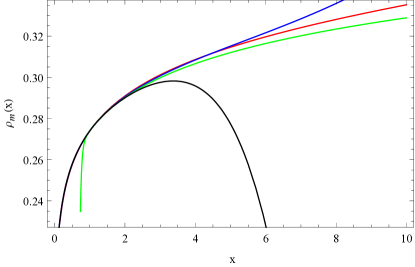
Figure 1: Plot for variation of shifted exotic matter energy density $\rho_{m}(x)$ with redshift ($x$ for range $0$ to $10$). We assume $\eta=0.001$, $\varepsilon=0.02$, $\alpha=1.2$ and $\beta=1.2,-1.2,0.2,-0.2$ for $\bar{\Omega}^{0}_{m}\simeq 0.274$ and $\bar{\Omega}^{0}_{\lambda}\simeq 0.725$. The red, green, blue and black curves correspond to $\beta=1.2,-1.2,0.2$ and $-0.2$, respectively.

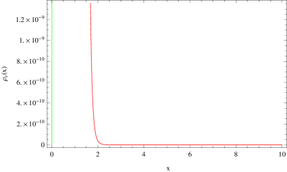
Figure 2: Variation of shifted radiation energy density $\rho_{r}(x)$ with redshift ($x$ for range $0$ to $10$). We assume $\eta=0.001$, $\varepsilon=0.02$, $\alpha=1.2$ and $\beta=1.2$ and $-1.2$ for $\bar{\Omega}^{0}_{r}\simeq 0.00005$. The red and green curves stand for $\beta=1.2$ and $-1.2$ respectively.

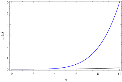
Figure 3: Variation of shifted radiation energy density $\rho_{r}(x)$ with redshift ($x$ for range $0$ to $10$). We assume $\eta=0.001$, $\varepsilon=0.02$, $\alpha=1.2$ and $\beta=0.2$ and $-0.2$ for $\bar{\Omega}^{0}_{r}\simeq 0.00005$. The blue and black curves refer to $\beta=0.2$ and $-0.2$, respectively.

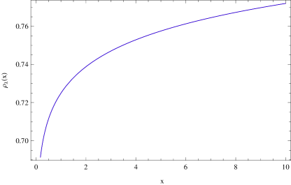
Figure 4: Variation of energy density for shifted cosmological parameter $\rho_{\lambda}(x)$ with redshift ($x$ for range $0$ to $10$). We assume $\eta=0.001$, $\varepsilon=0.02$, $\alpha=1.2$ for $\bar{\Omega}^{0}_{\lambda}\simeq 0.725$. The plot is independent of the chosen values of $\beta$

III $O_{m}(x)$ diagnostics for interaction

Recently, Sahni et al a6 introduced the redshift dependent function

$$O_{m}(x)=\frac{E^{2}(x)-1}{x^{3}-1}$$ (25)

where $E(x)=H(x)/H_{0}$ is the normalized Hubble function

$$E^{2}(x)=(1+M)\bar{\Omega}^{0}_{\lambda}x^{3\varepsilon/1+\alpha}+(1-N)\bar{\Omega}^{0}_{r}x^{4+3\varepsilon/1-\beta}$$

$$+(\bar{\Omega}^{0}_{m}-M\bar{\Omega}^{0}_{\lambda}+N\bar{\Omega}^{0}_{r})x^{\eta}$$ (26)

where the constants $M$ and $N$ are respectively given as

$$M=\frac{3\varepsilon\alpha}{3\varepsilon-\eta-\eta\alpha}$$ (27)

$$N=\frac{\beta(4+3\varepsilon)}{4+3\varepsilon-\eta+\eta\beta}$$ (28)

and $\bar{\Omega}^{0}$ is the present density parameter in the spatially flat $(k=0)$ universe.

Figure 5: Normalized Hubble parameter $E^{2}(x)$ with redshift ($x$ for range $0$ to $10$). We assume $\eta=0.001$, $\varepsilon=0.02$, $\alpha=1.2$ and $\beta=1.2$ and $-1.2$ for $\bar{\Omega}^{0}_{m}\simeq 0.274$ and $\bar{\Omega}^{0}_{\lambda}\simeq 0.725$. Blue and green curves correspond to $\beta=1.2$ and $-1.2$, respectively.

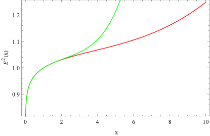
Figure 6: Normalized Hubble parameter $E^{2}(x)$ with redshift ($x$ for range $0$ to $10$). We assume $\eta=0.001$, $\varepsilon=0.02$, $\alpha=1.2$ and $\beta=0.2$ and $-0.2$ for $\bar{\Omega}^{0}_{m}\simeq 0.274$ and $\bar{\Omega}^{0}_{\lambda}\simeq 0.725$. Green and red curves refer to $\beta=0.2$ and $-0.2$, respectively.

In our scenario (perturbation + interaction) the $O_{m}(x)$-diagnostics is given as

$$O_{m}(x)=\frac{Ax^{3\varepsilon/1+\alpha}+Bx^{4+3\varepsilon/1-\beta}+Cx^{\eta}-1}{x^{3}-1}$$ (29)

where

$$A=(1+M)\bar{\Omega}_{\lambda}^{0},$$

$$B=(1-N)\bar{\Omega}_{r}^{0}$$

and

$$C=\bar{\Omega}_{m}^{0}+N\bar{\Omega}_{r}^{0}-M\bar{\Omega}_{\lambda}^{0}.$$

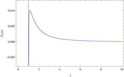
Figure 7: Plot of $O_{m}(x)$-diagnostics with redshift ($x$ for range $0$ to $10$). We assume $\eta=0.001$, $\varepsilon=0.02$, $\alpha=1.2$ and $\beta=1.2$ and $-1.2$ for $\bar{\Omega}^{0}_{\lambda}\simeq 0.725$, $\bar{\Omega}^{0}_{m}\simeq 0.274$ and $\bar{\Omega}^{0}_{r}\simeq 0.00005$. The plot is independent of the chosen values of $\beta$.

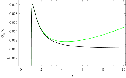
Figure 8: Plot of $O_{m}(x)$-diagnostics with redshift ($x$ for range $0$ to $10$). We assume $\eta=0.001$, $\varepsilon=0.02$, $\alpha=1.2$ and $\beta=-0.2$ and $-0.2$ for $\bar{\Omega}^{0}_{\lambda}\simeq 0.725$, $\bar{\Omega}^{0}_{m}\simeq 0.274$ and $\bar{\Omega}^{0}_{r}\simeq 0.00005$. Green and black curves are plotted for $\beta=0.2$ and $-0.2$ respectively.

The difference of the squares of the normalized Hubble parameter $E^{2}(x)$ at two different redshifts $x_{i}$ and $x_{j}$ is given as

$$\Delta E^{2}(x_{i},x_{j})=\bar{M}\bar{\Omega}^{0}_{\lambda}(x_{i}^{3\varepsilon/1+\alpha}-x_{j}^{3\varepsilon/1+\alpha})+$$

$$\bar{N}\bar{\Omega}^{0}_{r}(x_{i}^{4+3\varepsilon/1-\beta}-x_{j}^{4+3\varepsilon/1-\beta})+\chi(x_{i}^{\eta}-x_{j}^{\eta})$$ (30)

where

$$\Delta E^{2}(x_{i},x_{j})=E^{2}(x_{i})-E^{2}(x_{j}).$$

Measuring the values of $\Delta E^{2}(x_{i},x_{j})$ from observations we can estimate the proportionality constants.

Table 1: First column shows the Hubble parameter $H(z)$. Second and third columns give the redshifts $z_{i}$ and $x_{i}=1+z_{i}$ where $i=1,2,3,4$.

$H(z)$	$z_{i}$	$x_{i}$
$69\pm 12$	0.1	1.1
$95\pm 17$	0.4	1.4
$168\pm 17$	1.3	2.3
$202\pm 40$	1.75.	2.75

We further take a set of values $H(z)$ at different redshifts given in Table 1 c1 . From these values, we obtain six non-linear equations. Thus, from (30) with $H_{0}=73.8\pm 2.4\approx 73.8$ c2 we obtain six values of $\Delta E^{2}(x_{i},x_{j})$ mentioned in Table 2.

Table 2: First column gives the difference of squared normalized Hubble parameter $\Delta E^{2}(x_{i},x_{j})$, Second column is its numeric value and third column is pairs of redshifts, where $i=1,2,3,4$ and $j=1,2,3,4$.

$\Delta E^{2}(x_{i},x_{j})$	Numeric Value	$(x_{i},x_{j})$
$\Delta E^{2}(x_{1},x_{2})$	$-0.783$	$(1.1,1.4)$
$\Delta E^{2}(x_{1},x_{3})$	$-4.308$	$(1.1,2.3)$
$\Delta E^{2}(x_{1},x_{4})$	$-6.618$	$(1.1,2.75)$
$\Delta E^{2}(x_{2},x_{3})$	$-3.525$	$(1.4,2.3)$
$\Delta E^{2}(x_{2},x_{4})$	$-5.835$	$(1.4,2.75)$
$\Delta E^{2}(x_{3},x_{4})$	$-2.310$	$(2.3,2.75)$

With the help of these two Tables we have following six non-linear equations for $\Delta E^{2}(x_{i},x_{j})$

$$A_{1}[(1.1)^{3\varepsilon/1+\alpha}-(1.4)^{3\varepsilon/1+\alpha}]+$$

$$A_{2}[(1.1)^{4+3\varepsilon/1-\beta}-(1.4)^{4+3\varepsilon/1-\beta}]$$

$$+C[(1.1)^{\eta}-(1.4)^{\eta}]=-0.783$$ (31)

$$A_{1}[(1.1)^{3\varepsilon/1+\alpha}-(2.3)^{3\varepsilon/1+\alpha}]+$$

$$A_{2}[(1.1)^{4+3\varepsilon/1-\beta}-(2.3)^{4+3\varepsilon/1-\beta}]$$

$$+C[(1.1)^{\eta}-(2.3)^{\eta}]=-4.308$$ (32)

$$A_{1}[(1.1)^{3\varepsilon/1+\alpha}-(2.75)^{3\varepsilon/1+\alpha}]+$$

$$A_{2}[(1.1)^{4+3\varepsilon/1-\beta}-(2.75)^{4+3\varepsilon/1-\beta}]$$

$$+C[(1.1)^{\eta}-(2.75)^{\eta}]=-6.618$$ (33)

$$A_{1}[(1.4)^{3\varepsilon/1+\alpha}-(2.3)^{3\varepsilon/1+\alpha}]+$$

$$A_{2}[(1.4)^{4+3\varepsilon/1-\beta}-(2.3)^{4+3\varepsilon/1-\beta}]$$

$$+C[(1.4)^{\eta}-(2.3)^{\eta}]=-3.525$$ (34)

$$A_{1}[(1.4)^{3\varepsilon/1+\alpha}-(2.75)^{3\varepsilon/1+\alpha}]+$$

$$A_{2}[(1.4)^{4+3\varepsilon/1-\beta}-(2.75)^{4+3\varepsilon/1-\beta}]$$

$$+C[(1.4)^{\eta}-(2.75)^{\eta}]=-5.835$$ (35)

$$A_{1}[(2.3)^{3\varepsilon/1+\alpha}-(2.75)^{3\varepsilon/1+\alpha}]+$$

$$A_{2}[(2.3)^{4+3\varepsilon/1-\beta}-(2.75)^{4+3\varepsilon/1-\beta}]$$

$$+C[(2.3)^{\eta}-(2.75)^{\eta}]=-2.310$$ (36)

where

$$A_{1}=\bar{M}\bar{\Omega}^{0}_{\lambda},$$

$$A_{2}=\bar{N}\bar{\Omega}^{0}_{r}.$$

IV $O_{m}3(x)$ diagnostics and Statefinders

The two point $O_{m}(x)$-diagnostics may be defined asa7

$$O_{m}(x_{2},x_{1})=\frac{E^{2}(x_{2})-E^{2}(x_{1})}{x_{2}^{3}-x_{1}^{3}}$$ (37)

and $3$-point $O_{m}(x)$-diagnostics as

$$O_{m}(x_{3},x_{2},x_{1})=\frac{O_{m}(x_{2},x_{1})}{O_{m}(x_{3},x_{1})}.$$ (38)

Using (37) and (38) we have $O_{m}3(x)$-diagnostic

$$O_{m}(x_{3},x_{2},x_{1})=\frac{E^{2}(x_{2})-E^{2}(x_{1})}{x_{2}^{3}-x_{1}^{3}}.\frac{x_{3}^{3}-x_{1}^{3}}{E^{2}(x_{3})-E^{2}(x_{1})}$$ (39)

$E^{2}(x_{3})$, $E^{2}(x_{2})$ and $E^{2}(x_{1})$ can be calculated from (26) at three different redshifts. We would take up this study in future. Here, we use the statefinders for constraining the interaction.

In addition to the cosmological constant several other candidates for dark energy (quintom, quintessence, brane-world, modified gravity etc., e.g. a8 ) have been proposed. To differentiate different models of dark energy Sahni et.al a9 proposed statefinder diagnostics based on dimensionless parameters $(r,s)$ which are the functions of scale factor and its time derivative. These parameters are define as

$$r=\frac{\dddot{a}}{aH^{3}}$$

and

$$s=\frac{r-1}{3(q-\frac{1}{2})}$$

with deceleration parameter

$$q=-\frac{\ddot{a}}{aH^{2}}$$

Thus, re-writng the statefinders as,

$$r=\frac{\ddot{H}}{H^{3}}+\frac{3\dot{H}}{H^{2}}+1$$ (40)

$$s=-\frac{2}{3(3H^{2}+2\dot{H})}\left[\frac{\ddot{H}}{H}+3\dot{H}\right].$$ (41)

Considering for interaction + perturbation scenario the statefinder parameters may be calculated as from (26). Let

$$H^{2}(x)=H^{2}_{0}y_{0}$$ (42)

where

$$y_{0}=Ax^{3\varepsilon/1+\alpha}+Bx^{4+3\varepsilon/1-\beta}+Cx^{\eta}$$ (43)

$$r=\frac{y_{2}\dot{x}^{2}}{2H^{2}_{0}y^{2}_{0}}+\frac{y_{1}\dot{x}\ddot{x}}{2H^{2}_{0}y^{2}_{0}}-\frac{y^{2}_{1}\dot{x}^{2}}{2H^{2}_{0}y^{3}_{0}}(1-3H^{2}_{0}y_{0})+1$$ (44)

where

$$y_{1}=A\left(\frac{3\varepsilon}{1+\alpha}\right)x^{\frac{3\varepsilon}{1+\alpha}-1}$$

$$+B\left(\frac{4+3\varepsilon}{1-\beta}\right)x^{\frac{4+3\varepsilon}{1-\beta}-1}$$

$$+C\eta x^{\eta-1}$$ (45)

$$y_{2}=A\left(\frac{3\varepsilon}{1+\alpha}\right)\left(\frac{3\varepsilon-\alpha-1}{1+\alpha}\right)x^{\frac{3\varepsilon}{1+\alpha}-2}$$

$$+B\left(\frac{4+3\varepsilon}{1-\beta}\right)\left(\frac{3+3\varepsilon+\beta}{1-\beta}\right)x^{\frac{4+3\varepsilon}{1-\beta}-2}$$

$$+C\eta(\eta-1)x^{\eta-2}$$ (46)

From (44),(45) and (46) we can find the other statefinder parameter $s$ defined by (41) as given below

$$s=\zeta\left[\frac{H_{0}y_{2}\dot{x}^{2}}{y^{1/2}_{0}}+\frac{H_{0}y_{1}\dot{x}\ddot{x}}{y^{1/2}_{0}}-\frac{y_{1}\dot{x}}{y_{0}}+3H^{2}_{0}y_{1}\dot{x}\right]$$ (47)

where $\zeta$ given as

$$\zeta=-\frac{1}{3(3H^{3}_{0}y^{3/2}_{0}+2H^{2}_{0}y_{1}\dot{x})}.$$ (48)

For non-interacting model i.e., $\alpha=0$ and $\beta=0$ and in the absence of perturbation these turn out to be the same as in $\Lambda$CDM model $(r=1,s=0)$ for $(w_{\lambda}=-1)$ and $(w_{m}=0)$ with negligible contribution of radiation.

V Discussion

We argue that the contributions from the recent acceleration of the universe must generate the tensor fluctuations in a way similar to early inflation. It would amplify the tensor-to-scalar ratio. In fact, being robust and of recent and much longer duration this may explain the high value of $r$ recently observed by BICEP2, since it must represent a the sum of inflationary as well as well as the post-inflationary current acceleration. We have used the single tachyonic scalar field which splits due to some unknown (apparently Higgs-like) mechanism into three components (cosmological constant, radiation and dust matter) which interact to achieve a thermodynamical equilibrium. The interaction among the components at present may boost the tensor-to-scalar amplitude ratio caused by the early inflation and must appear as the enhanced signature beyond the bounds set by the Planck observations. The entire evolution of the universe arises from this process of interaction. Due to consideration of radiation in this field the dust matter appears with negative energy. A small perturbation allowed in EoS of cosmological constant changes its status from a true cosmological constant to a shifted cosmological parameter. Similarly, status of radiation and dust matter changes to shifted radiation and shifted exotic matter. With the perturbation shifted exotic matter gains non-zero negative pressure which also helps (along with dark energy) in the accelerated expansion of the universe. Total energy of field stays conserved but the field components mutually interact with interaction strength parameter $Q$ resulting in local violation of energy conservation. The interaction reflects in diagnostics with our choice of interaction strengths which are constrained by the astrophysical data of Hubble parameter at different redshifts chosen ( $z=0.1,0.4,1.3$ and $1.75$) (albeit a narrower range of redshifts would be more useful in determining dynamics at an epoch). The $O_{m}3(x)-$ diagnostics and Statefinder parameters may be further explored for interaction $+$ perturbation model to check the important constraints.

References

(1) P. A. R. Ade et al., B. Collaboration (2014), arxiv:1403.3985.
(2) P. A. R Ade et al., Planck Collaboration (2013), arxiv:1303.5082.
(3) A. G. Riess et al., Astron.J. 116, 1009 (1998).
(4) S. Perlmutter el al., Astrophys.J. 517, 565(1999).
(5) B. P. Schmidt et al., Astrophys.J. 507, 46(1998).
(6) M. M. Verma and S. D. Pathak, Int. J. Theor. Phys. 10773 (2012).
(7) I. Dymnikova and M. Khlopov, Mod. Phys. Lett. A. 15, 2305-2314 (2000).
(8) I. Dymnikova and M. Khlopov, Eur. Phys. J. C 20, 139-146 (2001).
(9) A. Sen, JHEP 0204, 048 (2002); JHEP 0207, 065 (2002); Mod. Phys. Lett. A. 17, 1797 (2002).
(10) E. S. Reich, NATURE (London) Vol. 483, 132 8 March 2012.
(11) R. M. Lutchyn, J. D. Sau and S. D. Sarma, Phys. Rev. Lett. 105, 077001 (2010).
(12) M. M. Verma and S. D. Pathak, Astrophys. Space Sci. 344, 505(2013).
(13) L. Amendola, Phys. Rev. D 62, 043511(2000).
(14) W. Zimdahl and D. Pavon, Phys. Lett. B 521, 133(2011).
(15) M. M. Verma, Astrophys. Space Sci. 330, 101(2010).
(16) M. M. Verma, Texas Symposium on Relativistic Astrophysics–TEXAS 2010, December 06-10, 2010, Heidelberg, Germany, (Proceedings of Science, 218, (2010). SISSA, Italy).
(17) L. P. Chimento, Phys. Rev. D 81, 043525(2010).
(18) J. H. He, B. Wang and P. Zhang, Phys. Rev. D 80, 063530(2009).
(19) B. Wang, Y. G. Gong and E. Abdalla, Phys. Lett. B 624, 141(2005).
(20) S. D. Campo, R. Herrera and D. Pavon, IJMP D Vol.20, 4 561(2011).
(21) H. Wei and R. G. Cai, Phys. Rev. D 71, 043504(2005).
(22) H. Wei and S. N. Zhang, Phys. Lett. B 644, 7(2007).
(23) V. Sahni, A. Shafieloo and A. A. Starobinsky, Phys. Rev. D 78, 103502 (2008).
(24) D. Stern, et al., JCAP 1002 008 (2010).
(25) A. G. Riess et al., Astrophys. J. 730, 119 (2011).
(26) A. Shafieloo, V. Sahni and A. A. Starobinsky, Phys. Rev. D 86, 103527 (2012).
(27) Y. Cai, E. N. Saridakis, M. R. Setare and J. Xia, Phys. Rept. 493, 1 (2010).
(28) V. Sahni, T. D. Saini, A. A. Starobinsky, and U. Alam, JETP Lett. 77, 201 (2003).