HU-Mathematik: 2013-23 HU-EP-13/75 DCPT-13/49

Local integrands for the five-point amplitude in planar N=4 SYM up to five loops

Raquel G. Ambrosio^a, Burkhard Eden^a,
Timothy Goddard^b, Paul Heslop^b, Charles Taylor^c

^a Institut für Mathematik und Physik, Humboldt-Universität,
Zum großen Windkanal 6, 12489 Berlin ^b Mathematics department, Durham University, Durham DH1 3LE, UK ^c 8 Cherryl House, Seymour Gardens, Sutton Coldfield, West Midlands, B74 4ST, UK

Abstract

Integrands for colour ordered scattering amplitudes in planar N=4 SYM are dual to those of correlation functions of the energy-momentum multiplet of the theory. The construction can relate amplitudes with different numbers of legs.

By graph theory methods the integrand of the four-point function of energy-momentum multiplets has been constructed up to six loops in previous work. In this article we extend this analysis to seven loops and use it to construct the full integrand of the five-point amplitude up to five loops, and in the parity even sector to six loops.

All results, both parity even and parity odd, are obtained in a concise local form in dual momentum space and can be displayed efficiently through graphs. We have verified agreement with other local formulae both in terms of supertwistors and scalar momentum integrals as well as BCJ forms where those exist in the literature, i.e. up to three loops.

Finally we note that the four-point correlation function can be extracted directly from the four-point amplitude and so this uncovers a direct link from four- to five-point amplitudes.

1 Introduction

There has been a great deal of recent progress in calculating scattering amplitudes of the maximally supersymmetric non-abelian Yang-Mills theory in four dimensions, ${\cal N}=4$ SYM. In particular, interesting structures enabling new results have been found for the amplitude integrand both in the planar limit as well as for the full non-planar theory. Perturbative calculations by Feynman graphs are complicated due to the vast number of contributing diagrams, which makes it difficult to construct even the integrand. To evaluate the integrals is, of course, the hardest step — which we will not attempt to take in this work — but it will obviously be facilitated by finding simple concise forms of the integrands.

There have been three main methods used for generating integrands. (Generalised) unitarity is the most widespread technique [1, 2, 3, 4]. Here one equates the leading singularities of an ansatz — consisting of a sum of independent graphs with arbitrary coefficients — with those of the amplitude, which will fix all freedom. There are various criteria as to which graphs should occur in the ansatz: in the planar limit one uses dual conformal invariance [5, 6, 7, 8, 9], whereas in the full non-planar theory one can use the colour-kinematics duality [10, 11]. This technique has been used to obtain the four-point amplitude up to five-loops (planar [12, 13, 14, 15] and nonplanar [16, 17, 18, 19]), the five-point amplitude to three-loops [20, 21, 22] and six-point amplitude to two loops [23, 24].

Second, one may employ a recursion relation determining higher loop amplitudes in terms of lower ones [25]. The original BCFW [26] recursion decomposed higher-point tree-level amplitudes into products of three-point amplitudes, but in a striking development this technique has been generalised to loop integrands [25]. The use of these on-shell methods, in particular in terms of momentum twistor variables, yields relatively compact expressions where Feynman graph calculations would often result in millions of terms. By construction, BCFW recursion leads to non-local integrands, i.e. individual terms have poles which are not of $1/p^{2}$ type. Yet, the existence of the Feynman graph method guarantees the cancellation of such spurious singularities in the sum of all terms. It remains a formidable problem though, to find simple local forms for the BCFW output, since the recursion procedure — although much more concise than any direct graph calculation — does fan out considerably for higher-loop integrands (although much progress has been made towards a resolution of this problem [27]). So far explicit formulae for local integrands via this method are available for MHV $n$-point amplitudes up to three loops and NMHV $n$-point amplitudes up to two loops [25, 28].

Third, another less widely known but extremely powerful technique starts from an ansatz, but now fixes the coefficients by implementing the exponentiation of infrared singularities at the level of the integrand by asserting that the log of the amplitude should have a reduced singularity [29]. This method has been used to obtain the four-point amplitude to seven loops [29], and has been shown to determine the $n$-point amplitudes at two and three loops for any $n$ [30].

Both this method and generalised unitarity customarily use graphs with local integrands. In addition, the trial graphs used in generalised unitarity methods typically contain only Lorentz products, with any parity odd structures being in the external variables only.

Planar scattering amplitudes in ${\cal N}=4$ are dual to polygonal Wilson loops with light-like edges [31, 32, 33, 23, 34]. It has recently been shown that both sides of this duality can be generated from $n$-point functions of the energy-momentum tensor multiplet of the theory [35, 36, 37, 38, 39] To this end, the operators in such an $n$-point correlator are put on the vertices of an $n$-gon with light-like edges. The relation between correlation functions and Wilson loops, which are also defined on configuration space, is rather direct [36] and can be made supersymmetric [40, 41, 42]. On the other hand, the connection between energy-momentum correlation functions and amplitudes is conceptually not well understood, while it provides a fully supersymmetric integrand duality which exactly reproduces the BCFW based loop integrands [37, 38, 39, 42]. The counterpart of the disc planarity of amplitudes is planarity on the sphere for the correlation functions. More specifically, the correlation functions yield the square of the amplitude integrands; here the two discs are quite literally welded together like the hemispheres of a ball touching at the equator.

The component operators in the energy momentum tensor multiplet are dual to supergravity states on AdS₅ in the AdS/CFT correspondence [43]. In the next section we will use superspace to package all the component operators into one superoperator; he we rather write ${\cal O}_{\Lambda}(x)$ where $\Lambda$ is simply a schematic label describing the precise component in question.

Two- and three-point functions of these operators can be shown to be protected from quantum corrections. As the first non-trivial objects the four-point functions have been intensely studied both at weak coupling in field theory perturbation theory and at strong coupling exploiting the AdS/CFT duality. The loop corrections to these four-point function take a factorised form [44]:

$$\langle{\cal O}_{\Lambda_{1}}{\cal O}_{\Lambda_{2}}{\cal O}_{\Lambda_{3}}{\cal O}_{\Lambda_{4}}\rangle\,=\,\langle{\cal O}_{\Lambda_{1}}{\cal O}_{\Lambda_{2}}{\cal O}_{\Lambda_{3}}{\cal O}_{\Lambda_{4}}\rangle_{\mathrm{tree}}+{\cal I}_{{\Lambda}_{1}{\Lambda}_{2}{\Lambda}_{3}{\Lambda}_{4}}(x_{i})\times\,f(x_{i};a)$$ (1)

In this equation ${\cal I}$ does not depend on the ’t Hooft coupling $a=g^{2}N/(4\pi^{2})$ but does depend on the particular component operators in question; whereas all the non-trivial coupling dependence lies in the single function $f$. We have $\ell$-loop integrands $f^{(\ell)}(x_{1},\dots x_{4+\ell})$ via

$$f(x_{i};a) =\sum_{\ell=1}^{\infty}{a^{\ell}\over\ell!}\,\int d^{4}x_{5}\dots d^{4}x_{4+\ell}\;f^{(\ell)}(x_{1},\dots,x_{4+\ell})$$ (2)

The one- and two-loop contributions were computed using supergraphs [45, 46]. In [47, 48] it was shown that all the loop integrands have an unexpected (hidden) symmetry permuting internal and external variables:

$$f^{(\ell)}(x_{1},\dots x_{4+\ell})=f^{(\ell)}(x_{\sigma_{1}},\dots x_{\sigma_{4+\ell}})\qquad\qquad\forall\,\sigma\in S_{4+\ell}\ .$$ (3)

The $S_{4+\ell}$ invariance together with conformal covariance ($f^{(\ell)}$ must have conformal weight 4 at each of the $4+\ell$ points), the absence of double propagator terms (which follows from an OPE analysis), and planarity of the corresponding graph beyond 1 loop, constrains the number of undetermined parameters in an ansatz of this type so severely that up to three loops there is only one term in the ansatz. Indeed even at higher loops it was possible to determine $f^{(l)}$ up to $l=6$ in combination with the aforementioned criteria about the exponentiation of infrared singularities [47, 48].

We note that any single term in $f^{(\ell)}$ has numerator and denominator composed of squared distances $x_{ij}^{2}$. The graph obtained by regarding the denominator factors as edges is called an “$f$-graph” below. These provide an exceptionally compact way to display the result, for example we display the full four-point correlator up to five-loops compactly via $f$-graphs below in (LABEL:eq:6). In diagrams we denote the numerator factors by dashed lines.

At four-points the amplitude/correlation function duality relates the four-point light-like limit of $f(x_{i};a)$ to the four-point amplitude $M_{4}(x_{i};a)$ (divided by the tree amplitude) in dual momentum space $p_{i}\,=\,x_{i}-x_{i+1}$ :

$$1+2\sum_{\ell\geq 0}a^{\ell}\,F_{4}^{(\ell)}\ =\ \bigl{(}M_{4}(x_{i};a)\bigr{)}^{2}$$ (4)

where

$$F_{4}^{(\ell)}(x_{1},x_{2},x_{3},x_{4})\ =\ \text{external factor }\times\lim_{\begin{subarray}{c}x_{i\,i+1}^{2}\rightarrow 0\\ (\text{mod }4)\end{subarray}}\int d^{4}x_{5}\dots d^{4}x_{4+\ell}\,{f^{(\ell)}\over\ell!}\ .$$ (5)

and where the external factor is simply ${x^{2}_{13}x^{2}_{24}}\prod_{1\leq i<j\leq 4}x^{2}_{ij}$. Graphically the light-like limit on the l.h.s. corresponds to selecting all possible 4-cycles in the $f$-graph (corresponding to the four external points) which then splits the planar f-graph into two disc planar pieces corresponding to the product of two amplitudes.

The interaction between four-point correlation functions and amplitudes has been the focus of much work in this direction [47, 48, 49]. Indeed one can use this relation in reverse to read off the correlation function from the amplitude and to this end $f^{(7)}$ has recently been obtained [50] using the corresponding seven-loop amplitude [29].

However, less use has been made of the fact that the very same four-point correlation function is related to particular combinations of higher point amplitudes. This remarkable feature takes place simply due to the fact that loop corrections of correlation functions are correlation functions with the Lagrangian inserted. But the Lagrangian is itself an operator in the energy-momentum supermultiplet and therefore we find that loop corrections of $n$-point correlators of energy-momentum multiplets are given by certain higher point correlators of energy-momentum multiplets. These are then in turn related to higher point amplitudes via the amplitude/correlation functions duality. The details of how this works will be derived in the next section, but here let us simply note the result

$$\sum_{\ell\geq 0}{a^{\ell}}{F_{5}^{(\ell)}}\ =\ M_{5}\,\overline{M}_{5}\ ,$$ (6)

where $F_{5}^{(\ell)}(x_{1},\dots,x_{5})$ is constructed from the four-point correlator integrands $f^{(\ell)}$:

$$F_{5}^{(\ell)}(x_{1},\dots,x_{5}):=\text{external factor}\times\lim_{\begin{subarray}{c}x_{i\,i+1}^{2}\rightarrow 0\\ (i=1\dots 5)\end{subarray}}\int d^{4}x_{6}\dots d^{4}x_{5+\ell}{}{f^{(\ell+1)}\over\ell!}\ ,$$ (7)

where here the external factor is $1/f^{(1)}=\prod_{1\leq i<j\leq 5}x^{2}_{ij}$. $M_{5}$ is the 5-point MHV amplitude (divided by tree-level) One can readily see the similaity between (6) and the four-point relation (4). So the five-point light-like limit of the four-point correlator $f$-graphs yields the above combination of the five-point amplitude, whereas the four-point lightlike limit of the same correlator yields the four-point amplitude: both the four- and five-point amplitudes are contained in the four-point correlator!

Even so, how can the single equation (6) uniquely determine $M_{5}$? The perturbative expansion of the r.h.s. contains the parity even part $M_{5}+\overline{M}_{5}$ (by choosing the leading 1 in either factor) but beyond it also all possible product terms. Now, the (sphere) planar part of the correlator integrand on the l.h.s. of the equation breaks into classes of terms in exactly the same way. Taking the five-point light-like limit corresponds to chosing a 5-cycle on the $f$-graph (as opposed to a 4-cycle when considering the four-point amplitude) which splits the $f$-graph into two disc planar pieces; the $\ell$-loop integrand contains terms corresponding to a single $\ell$-loop integral as well as products of $m$-loop and $(\ell-m)$-loop integrals. The single equation (6) is therefore “stratified” into an over-determined system that turns out to be beautifully consistent.

The article is organised as follows: In Section 2 we demonstrate how the step from four-point to five-point integrands is taken. The resulting equation is split into classes of products. As a first application we discuss why four-point graphs always appear in a symmetric sum over the position of their massive leg. Sections 3,4,5, discuss the one-, two- and higher-loop amplitudes. Our main result — a local form of the complete four-loop amplitude — is given in Section 6. Furthermore, with the publication we include computer readable files containing also the complete five-loop and the parity even sector of the six-loop integrand in a local form. In a final section of the actual text we discuss the relation to other forms of the amplitude where available in the literature. Some appendices discuss technical details.

2 The amplitude₅/correlator₄ duality

2.1 Deriving the duality

We here derive and give more detail to some of the main formulae of the introduction. The starting point is the correlator/amplitude duality [35, 36, 37, 38, 42, 39]. To make the full duality precise we use superspace to package together component fields. The components of the energy-momentum tensor multiplet, denoted ${\cal O}_{\Lambda}(x)$ in the introduction, can all be assembled into a single superfield ${\cal O}(x,\rho,\bar{\rho},y)=\mathrm{Tr}(W^{2})$ where the trace is over the $SU(N)$ gauge group, see [51, 52] and references therein. The field strength multiplet $W(x,\rho,\bar{\rho},y)$ lives on analytic superspace, which combines the Minkowski space variable $x$ with Grassmann odd coordinates $\rho,\bar{\rho}$ and $y$ coordinates which parametrise the internal symmetry of the ${\cal N}=4$ model. Likewise, amplitudes connected by supersymmetry can be packaged into a superamplitude customarily parametrised by momentum supertwistors [54, 55].

To obtain the full duality between any amplitude and any correlation function of these operators, one identifies light-like coordinate differences on the correlator side with the ingoing momenta of the amplitude according to $x_{i\,i+1}=p_{i}$ and puts $\bar{\rho}$ to zero at all points. The precise identification of the left handed Grassmann odd coordinates $\{\rho_{i}\}$ with the odd part of the momentum supertwistors $\{\chi_{i}\}$ is known [38, 39], but it is not needed here. Also, in the amplitude limits the $y$ coordinates will factor out.

Now let ${\cal G}_{n}$ denote the $n$-point function of energy-momentum multiplets ${\cal O}$. The amplitude/correlator duality [35, 36, 37, 38, 39] states that

$$\lim_{x_{i\,i+1}^{2}\rightarrow 0}\frac{{\cal G}_{n}}{{\cal G}_{n}^{\mathrm{tree}}}\,=\,({\cal M}_{n})^{2}\,,\qquad\bar{\rho}=0\,.$$ (8)

On the left hand side of this equation ${\cal G}_{n}$ is a superspace object containing component $n$-point correlators of any operator in the energy-momentum multiplet in one object (some of which are eliminated by sending $\bar{\rho}$ to zero); similarly on the right-hand side ${\cal M}_{n}$ contains all $n$-point amplitudes in the theory packaged in one superspace object: the superamplitude. To be precise, the symbol ${\cal M}_{n}$ in the last equation denotes the full superamplitude divided by the tree-level MHV amplitude, so the leading term is 1. Both sides of the equation have expansions both in powers of the odd superspace variables as well as in the coupling constant. Expanding in odd superspace variables we write

$${\cal G}_{n}\,=\,\sum_{k=0}^{n-4}G_{n;k}\,,\qquad{\cal M}_{n}\,=\,\sum_{k=0}^{n-4}M_{n;k}$$ (9)

where $G_{n;k}$ and $M_{n;k}$ contain $4k$ powers of the odd superspace variable. In particular, ${M}_{n;k}$ is the N^kMHV superamplitude.

By differentiation in the coupling constant it can be shown that

$$G_{n,k}^{(\ell)}\,=\,\frac{a^{\ell}}{\ell!}\prod_{i=1}^{\ell}\left(\int d^{4}x_{n+i}\,d^{4}\rho_{n+i}\right)G_{n+\ell;k+\ell}^{(0)}\,,\qquad\ell>0$$ (10)

where the superscript indicates the loop order. In other words, the $\ell$-loop correction to an energy-momentum $n$-point function is given by a superspace integral over a Born level correlator of the same type, just with correspondingly more points. This opens the possibility of considering various $n$-gon limits of the same correlator. We currently know very little about the correlation functions $G_{n;k}$ with $k<n-4$. On the other hand following [47, 48] we have a wealth of information about the “maximally nilpotent” case $k=n-4$. In this paper we exploit this mechanism to construct the five-point amplitude from the correlators $G^{(0)}_{n;n-4}$ that were originally elaborated for the higher-loop integrands of the four-point function. Specialising (10) to this case:

$$G_{4,0}^{(\ell)}\,=\,\frac{a^{\ell}}{\ell!}\prod_{i=1}^{\ell}\left(\int d^{4}x_{4+i}\,d^{4}\rho_{4+i}\right)G_{4+\ell;\ell}^{(0)}\,,\qquad G_{5,1}^{(\ell-1)}\,=\,\frac{a^{\ell-1}}{(\ell-1)!}\prod_{i=1}^{\ell-1}\left(\int d^{4}x_{5+i}\,d^{4}\rho_{5+i}\right)G_{4+\ell;\ell}^{(0)}\,.$$ (11)

According to [44, 45, 46, 47, 48] the Born level correlator with maximum $k=n-4$ (maximally nilpotent piece) has the form

$$G^{(0)}_{4+\ell;\ell}|_{\rho_{5}^{4}\dots\rho_{4+\ell}^{4}}\,=\,{\cal I}_{1234}\ \rho_{5}^{4}\ldots\rho_{4+\ell}^{4}\ f^{(l)}(x_{1},\ldots,x_{4+\ell})\,,$$ (12)

where

$${\cal I}_{1234}\,=\,\frac{2\,(N^{2}-1)}{(4\pi^{2})^{4}}\,(x_{12}^{2}x_{13}^{2}x_{14}^{2}x_{23}^{2}x_{24}^{2}x_{34}^{2})\,\left(\frac{y_{12}^{2}}{x_{12}^{2}}\frac{y_{23}^{2}}{x_{23}^{2}}\frac{y_{34}^{2}}{x_{34}^{2}}\frac{y_{14}^{2}}{x_{14}^{2}}\ x_{13}^{2}x_{24}^{2}+\,\ldots\right)\,$$ (13)

Here the dots indicate terms subleading in both the 4-gon $x_{12}^{2},x_{23}^{2},x_{34}^{2},x_{41}^{2}\,\rightarrow\,0$ and the 5-gon limit $x_{12}^{2},x_{23}^{2},x_{34}^{2},x_{45}^{2},x_{51}^{2}\,\rightarrow\,0$ which we are interested in.

The objects $f^{(\ell)}(x_{1},\dots x_{4+\ell})$, as explained in the introduction, are rational, symmetric in all $4+\ell$ variables, conformally covariant with weight 4 at each point and have no double poles. They can be displayed graphically via so-called $f$-graphs with vertices $x_{i}$ and edges denoting propagators $1/x_{ij}^{2}$. From 2-loops in the planar theory, the $f$-graphs will be planar (if we exclude numerator edges) $4+\ell$-point graphs with vertices of degree (or valency) four or more. Since we sum over all permutations of the vertices we need not label the graph - we sum over all possible labellings. Any vertex with degree $d$ greater that 4 must be accompanied by $d-4$ numerator lines to bring the total number of numerator lines minus denominator lines equal to 4 (corresponding to the fact that the $f^{(\ell)}$ has conformal weight 4 at each (external and internal) point) although we sometimes suppress the numerator lines for visual simplicity.

For illustration we here give the $f$-graphs to five-loops (ie the four-point correlator up to five-loops) and corresponding expressions up to three-loops:

$f^{(1)}$ =		$=\frac{1}{\prod_{1\leq i<j\leq 5}x_{ij}^{2}}\,,$
$f^{(2)}$ =		$=\frac{\frac{1}{48}\sum_{\sigma\in S_{6}}x_{\sigma_{1}\sigma_{2}}^{2}x_{\sigma_{3}\sigma_{4}}^{2}x_{\sigma_{5}\sigma_{6}}^{2}}{\prod_{1\leq i<j\leq 6}x_{ij}^{2}}$
$f^{(3)}$ =		$={{1\over 20}\sum_{\sigma\in S_{7}}x_{\sigma_{1}\sigma_{2}}^{4}x_{\sigma_{3}\sigma_{4}}^{2}x_{\sigma_{4}\sigma_{5}}^{2}x_{\sigma_{5}\sigma_{6}}^{2}x_{\sigma_{6}\sigma_{7}}^{2}x_{\sigma_{7}\sigma_{3}}^{2}\over\prod_{1\leq i<j\leq 7}x_{ij}^{2}}$

$f^{(4)}=$
$f^{(5)}=$

We see that $f^{(2)}$ has no remaining numerator terms (all three apparent numerator terms will be cancelled by the denominator) whereas $f^{(3)}$ has a single numerator line (coming from the $x^{4}_{\sigma_{1}\sigma_{2}}$ in the numerator which is only partially cancelled by the denominator.) This numerator edge will connect the two 5-valent vertices (shown in blue).

The one- and two-loop contributions were originally computed using supergraphs [45, 46] whereas the three-loop and higher were computed using the above symmetry considerations (as well as suppression of singularities for the coefficients) [47, 48].

Now according to (10), (11) we can consider this as either a four-point $\ell$-loop correlator or a five-point $\ell-1$ loop correlator (or of course a higher point correlator). First let us consider the four-point case (which is the one focussed on in previous work).

Four-point case

Eqns (10) and (12) lead directly to the factorised form

$${\cal G}_{4}|_{\bar{\rho}_{i}=0}\,=\,\langle{\cal O}_{1}{\cal O}_{2}{\cal O}_{3}{\cal O}_{4}\rangle_{\bar{\rho}_{i}=0}\,=\,{\cal G}^{\mathrm{tree}}_{4}|_{\bar{\rho}_{i}=0}+{\cal I}_{1234}(x_{i},\rho_{i},y_{i})\,f(x_{i};a)$$ (15)

which is just the superspace version of the factorisation mentioned in (1).

Now the four-point amplitude/correlator duality (8) gives the amplitude purely in terms of $f(x_{i};a)$ which we displayed in the introduction (4)

$$1+2\sum_{\ell\geq 0}a^{\ell}\,F_{4}^{(\ell)}\ =\ \bigl{(}M_{4;0}(x_{i};a)\bigr{)}^{2}$$ (16)

where

$$F_{4}^{(\ell)}\ =\ \text{external factor }\times\lim_{\begin{subarray}{c}x_{i\,i+1}^{2}\rightarrow 0\\ (\text{mod }4)\end{subarray}}\int d^{4}x_{5}\dots d^{4}x_{4+\ell}\,{f^{(\ell)}\over\ell!}\ .$$ (17)

Five-point case

Let us instead now consider (12) as the $\rho_{5}^{4}$ component of a five-point correlation function. For this special choice equation (10, 11, 12) can be written

$$G_{5;1}^{(l)}|_{\rho_{5}^{4}}\,=\,\frac{a^{\ell}}{\ell!}\prod_{i=6}^{5+\ell}\left(\int d^{4}x_{i}\,\right)G^{(0)}_{5;1}|_{\rho_{5}^{4}}\,\frac{f^{(l+1)}(x_{1},\ldots,x_{5+l})}{f^{(1)}(x_{1},\ldots,x_{5})}\,.$$ (18)

Now at five points there are MHV and NMHV amplitudes only and NMHV amplitudes are $\overline{\text{MHV}}$ amplitudes. Therefore

$$M_{5;1}\,=\,R_{12345}\,\overline{M}_{5;0}$$ (19)

where $R_{12345}$ is the five-point $R$ invariant [7, 55]. Since there is only one independent object we will henceforth drop the second subscript on $M_{5;0}$ and write $M_{5}$ instead. Furthermore, in the pentagon light-cone limit

$$\lim_{x_{i\,i+1}^{2}\rightarrow 0}\frac{G_{5;1}^{(0)}}{G_{5;0}^{\mathrm{tree}}}\,=\,2\,R_{12345}$$ (20)

as has been shown in [39]. The correlator amplitude duality (8) then implies

$$\lim_{x_{i\,i+1}^{2}\rightarrow 0}\frac{G_{5;1}}{G_{5}^{\mathrm{tree}}}\,=\,2\,R_{12345}\,M_{5}\,\overline{M}_{5}\,.$$ (21)

So combining (18, 21, 20) and dividing by $2\,R_{12345}|_{\rho_{5}^{4}}$ we obtain directly the relation between $f(x_{i};a)$ and the five-point amplitudes quoted in the introduction

$$\sum_{\ell\geq 0}{a^{\ell}}{F_{5}^{(\ell)}}\ =\ M_{5}\,\overline{M}_{5}\$$ (22)

with

$$F_{5}^{(\ell)}:=\lim_{\begin{subarray}{c}x_{i\,i+1}^{2}\rightarrow 0\\ (\text{mod }5)\end{subarray}}{}{f^{(\ell+1)}\over\ell!\,f^{(1)}}\ .$$ (23)

This is now an equation involving only spacetime points and will be the starting point for all that follows.

2.2 Refined duality

At the moment both sides of the equation contain the coupling constant. Expanding out the r.h.s. of (22) clearly gives

$$F_{5}^{(\ell)}=\sum_{m=0}^{\ell}M_{5}^{(m)}M_{5}^{(\ell-m)}\ .$$ (24)

But we can also say something more about the l.h.s. To do this we need to think a little more graphically than we have so far. In the previous subsection we reviewed $f$-graphs. Now to define $F_{5}^{(\ell)}$ we have done two things, firstly we have multiplied by the external factor $1/f^{(1)}=\prod_{1\leq i<j\leq 5}x_{ij}^{2}$ and secondly we have taken the light-like limit (see (4)). Multiplying by $\prod_{1\leq i<j\leq 5}x_{ij}^{2}$ corresponds to deleting all edges between points 1 to 5 (or adding numerator lines if no line exists). Taking the light-like limit means that any choice of external points 1,2,3,4,5 (recall that in the $f$-graph we sum over all choices) which are not connected cyclically via edges $[1,2],[2,3],\dots[5,1]$ will be surpressed. (Recall an edge $[i,j]$ represents $1/x_{ij}^{2}$.) So we only consider as external points, vertices connected in a five-cycle.

Now any cycle on a planar graph immediately splits the graph into two pieces. E.g. we can embed the graph on a sphere without crossing (since it is planar) and put the 5-cycle on the equator thus splitting the graph into a northern and a southern hemisphere. Alternatively, given an embedding of the graph on the plane, a 5-cycle splits the graph into an “inside” and an “outside” graph.

We can now classify terms in $F_{5}^{(\ell)}$ according to the number $m$ of points inside (or outside, whichever is smaller) the corresponding 5-cycle, as

$$F_{5}^{(\ell)}=\sum_{m=0}^{\lfloor\ell/2\rfloor}F_{5;m}^{(\ell)}\ .$$ (25)

The classification of terms in $F_{5}^{(\ell)}$ according to their graph structure is illustrated in Figure 1

	$=$		$\rightarrow$		$\in F_{5;0}^{(3)}$
	$=$		$\rightarrow$		$\in F_{5;1}^{(3)}$
$f$-graph with 5-cycle		“Inside”      “Outside”	$\times 1/f^{(1)}$

Figure 1: Figure illustrating graphically the classification of terms in $F_{5}^{(\ell)}$ into classes $F_{5;m}^{(\ell)}$. We start with a single $f$ graph (here contributing to $f^{(4)}$, see (LABEL:eq:6)). The correlator consists of summing over all possible labellings of this graph. Only terms where the external points $1,2,3,4,5$ are consecutively connected survive the light-like limit. Such a 5-cycle splits the $f$-graph into two pieces, an “inside” and an “outside” both of which are “disc planar” i.e. have the right planarity properties for amplitude graphs. The minimum of the number of vertices inside or outside the 5-cycle gives the value of $m$. Here we illustrate with two different 5-cycles (in thick red) on the same $f$-graph. The first has $m=0$ and the second $m=1$. On the right we give the corresponding amplitude graphs “inside” and “outside”.

A simple way of determining the value of $m$ for any given term in $F_{5}^{(\ell)}$ is to consider the reduced graph obtained by only considering edges between internal vertices (i.e. delete all external vertices). These will in general split into two disconnected groups of size $m$ and $\ell-m$.

In any case we see that $F_{5}^{(\ell)}$ naturally splits into the product of two graphs just as the duality with the amplitude suggests ($M_{5}\bar{M}_{5}$). Note that this split into products occurs only at the level of the denominator. We can and will see numerator terms linking the two product graphs. These will be considered later, but we mention here that such terms are directly related to parity odd terms in the amplitude.

In summary, then we expect a more refined duality relating specific terms of $F_{5}^{(\ell)}$ to specific products of amplitudes as

$$F_{5;m}^{(\ell)} =M_{5}^{(m)}\bar{M}_{5}^{(\ell-m)}+M_{5}^{(\ell-m)}\bar{M}_{5}^{(m)}\qquad m=0\dots\lfloor(\ell-1)/2\rfloor$$ (26)

$$F_{5;m}^{(\ell/2)} =M_{5}^{(\ell/2)}\bar{M}_{5}^{(\ell/2)}\qquad\ell\in 2{\mathbb{Z}}\ .$$

For this refined version of the duality to be true as stated we must be certain there can be no interaction between different terms (i.e. different values of $m$). The left hand side is clearly well-defined. The inside and outside of the 5-cycle on a planar f-graph is well-defined. On the right-hand side we need to ask if all terms in $M_{5}^{(\ell-m)}\bar{M}_{5}^{(m)}$ are uniquely identified by their topology as being $(\ell-m)$-loops times $m$-loop object. Stated differently, if a pentagon is drawn from points $1,2,3,4,5$ around $M_{5}^{(m)}$ say, can we also draw some or all of $M_{5}^{(\ell-m)}$ inside the pentagon without crossing. One can convince oneself that this is indeed not possible: $M_{5}^{(m)}$ contains at least four external vertices, any internal vertex of $M_{5}^{(\ell-m)}$ is connected to at least four external vertices and it is impossible to draw two such graphs inside the pentagon without crossing.

2.3 Four-point graphs appear symmetrically.

There is a simple all loop consequence of this duality which we mention here, namely that for 5-point amplitude graphs depending on only 4 external points (i.e. with one massive external momentum), the massive point must always appear symmetrically in all four places (where allowed).

Four-point amplitude graphs only arise in the parity even part of the amplitude. (The general form of the parity odd part will be discussed in later sections. Parity odd graphs always depend on all five points.) The parity even part of the amplitude is given by the $m=0$ sector of $F_{m}^{(\ell)}$ from (26). The $F_{m}^{(\ell)}$ sector has an “inside” and an “outside” as discussed in the previous section, and for $m=0$ the outside (say) has no vertices in it. The outside and inside must both be planar, but the inside contains a vertex which is not connected to any other point on the inside (apart from the two consecutive external points, around the pentagon) since it supposed to be a four-point graph. Since the $f$-graph has degree 4 or more at each point, this means there must be at least two lines attached to this point on the outside pentagon. The outside pentagon is then unique given planarity. In other words the “inside” and “outside” pentagons have the following form which combines into the $f$-graph on the right. In this picture, the blue edges and vertex represent the four-point amplitude graph in question (with conformal weight 1 at all four points)

See Figure 1 top row for an explicit example of this.

However, now we see the $f$-graph this four-point amplitude graph arises from, we can also see that there are a number of choices of 5 cycles all giving rise to the same amplitude graph but with the massive leg in different places:

The massive leg ($x_{14}^{2}$ in this case) shifts its position around the amplitude. We see that any four-point graph will appear symmetrically with respect to the position of its massive leg in the five-point amplitude. There is one slightly subtle apparent exception to this rule. That is the case where the original four-point amplitude has a numerator term $x_{14}^{2}$. In this case the numerator means there is an edge missing in the corresponding $f$-graph and since only one of the four 5-cycles does not pass through this missing edge, there is only one possible 5-cycle this time as illustrated:

However this is still consistent, since there is also only one allowed position for the massive leg: all other possibilities will be suppressed in the light-like limit by this numerator.

In summary, then we find that for any four point topology, the massive leg appears completely symmetrically. For this reason when giving our results we prefer to only display one representative of this class. We also of course have 5-point cyclic as well as dihedral symmetry and we only wish to display one term for all terms related by this symmetry.

We therefore define an operator which we call “cyc”, which does precisely this, namely cyc[“term”] denotes the sum over all terms related via cyclic or dihedral symmetry, or swapping of the position of the massive leg in the four-point case.

We will leave the precise definition of this operation to the appendix. But suffice it to say here that the argument of the operation cyc$[]$ always appears with weight 1 when expanding the result into inequivalent terms, i.e.

$$\text{cyc}[f(x_{1},x_{2},x_{3},x_{4})]=f(x_{1},x_{2},x_{3},x_{4})+\dots$$ (30)

where the dots denote different terms.

3 The one loop five-point amplitude from the correlator

Expanding out (6) to first order in the coupling (equivalent to considering (26) where $m$ can only take the value 0) gives

$$F_{5}^{(1)}\ =\ M_{5}^{(1)}+\overline{M}_{5}^{(1)}\ .$$ (31)

The left hand side of this is simply

$$F_{5}^{(1)}={\text{cyc}}\left[\frac{x^{2}_{13}x^{2}_{24}}{x^{2}_{16}x^{2}_{26}x^{2}_{36}x^{2}_{46}}\right]$$ (32)

which we recognise as the sum over 1 mass boxes. This is indeed twice the parity even part of the five-point one loop amplitude.

Having found the parity even part of the one loop amplitude from the correlator, we now ask if we can obtain the parity odd part? To do so let us go to next order.

Our refined duality equation (26) with $m=1,\,\ell=2$ gives

$$F^{(2)}_{5;1}\ =\ M_{5}^{(1)}\overline{M}_{5}^{(1)}\ .$$ (33)

So let’s check this. The contributions to $F_{5}^{(2)}$ which correspond to product graphs $m=1$ are given by:

$$F^{(2)}_{5;1}= \left(\frac{x^{4}_{13}x^{2}_{24}x^{2}_{25}}{x^{2}_{16}x^{2}_{17}x^{2}_{26}x^{2}_{27}x^{2}_{36}x^{2}_{37}x^{2}_{47}x^{2}_{56}}\ +\ {\text{cyclic in 1,2,3,4,5}}\ +\ x_{6}\leftrightarrow x_{7}\right)$$

$$+\frac{x^{2}_{13}x^{2}_{14}x^{2}_{24}x^{2}_{25}x^{2}_{35}x^{2}_{67}}{x^{2}_{16}x^{2}_{17}x^{2}_{26}x^{2}_{27}x^{2}_{36}x^{2}_{37}x^{2}_{46}x^{2}_{47}x^{2}_{56}x^{2}_{57}}$$

$$= \,\text{cyc}\left[\frac{x^{4}_{13}x^{2}_{24}x^{2}_{25}}{x^{2}_{16}x^{2}_{17}x^{2}_{26}x^{2}_{27}x^{2}_{36}x^{2}_{37}x^{2}_{47}x^{2}_{56}}+\frac{x^{2}_{13}x^{2}_{14}x^{2}_{24}x^{2}_{25}x^{2}_{35}x^{2}_{67}}{x^{2}_{16}x^{2}_{17}x^{2}_{26}x^{2}_{27}x^{2}_{36}x^{2}_{37}x^{2}_{46}x^{2}_{47}x^{2}_{56}x^{2}_{57}}\right]$$ (34)

Equating this to $M_{5}\bar{M}_{5}$, together with (32) gives us two equations for two unknowns, $M_{5}$ and $\bar{M}_{5}$ and we can thus solve for them. The equations are quadratic and so the solution involves a square root whose sign we will not be able to determine without more information.

The solution is simply

$$M_{5}^{(1)} ={1\over 2}\Big{(}F_{5}^{(1)}\pm\sqrt{(F_{5}^{(1)})^{2}-4F^{(2)}_{5;1}}\Big{)}$$ (35)

$$\overline{M}_{5}^{(1)} ={1\over 2}\Big{(}F_{5}^{(1)}\mp\sqrt{(F_{5}^{(1)})^{2}-4F^{(2)}_{5;1}}\Big{)}\ .$$ (36)

We have written the full parity even and odd 5-point ampitudes in terms of purely parity even objects (but involving a square root).

One can now ask if there is a better way of writing the parity odd part of this without using the square root, and indeed this is the case.

There is a unique parity odd conformally invariant tensor, which is easiest to see in the six-dimensional formalism reviewed in Appendix B. In this formalism it is clear that there is a unique parity odd conformally covariant object. It is a function of six points, $x_{1},\dots x_{6}$, each with weight 1 which we denote $\epsilon_{123456}$. It has a natural form in the six-dimensional formalism, but can be written in various different ways in standard four-dimensional formalism (see section B.1). In any case using this object one can show that the term inside the square root (thought of as an integrand product with integrand points $x_{6}$ and $x_{7}$ which are symmetrised) can be written in the more suggestive form

$$(F_{5}^{(1)})^{2}-4F^{(2)}_{5;1}=-{\epsilon_{123456}\over x^{2}_{16}x^{2}_{26}x^{2}_{36}x^{2}_{46}x^{2}_{56}}\times{\epsilon_{123457}\over x^{2}_{17}x^{2}_{27}x^{2}_{37}x^{2}_{47}x^{2}_{57}}\ .$$ (37)

To see this, use the identity

$$\epsilon_{123456}\times\epsilon_{123457}$$

$$= \text{cyc}\Big{[}2\,x_{67}^{2}x_{13}^{2}x_{24}^{2}x_{35}^{2}x_{14}^{2}x_{25}^{2}+x_{13}^{4}x_{24}^{2}x_{25}^{2}x_{46}^{2}x_{57}^{2}-x_{13}^{4}x_{24}^{4}x_{56}^{2}x_{57}^{2}-x_{13}^{2}x_{14}^{2}x_{24}^{2}x_{25}^{2}x_{36}^{2}x_{57}^{2}\Big{]}\,.$$ (38)

We then obtain our final result for the five-point amplitude to be

$$M_{5}^{(1)}=\frac{1}{2}\left({\cal I}_{1}^{(1)}+{\cal I}_{2}^{(1)}\right)\ .$$ (39)

The terms in this amplitude are displayed graphically in figure 2.

$$\mathcal{I}_{1}^{(1)} =\text{cyc}\left[\frac{x_{13}^{2}x_{25}^{2}}{x_{16}^{2}x_{26}^{2}x_{36}^{2}x_{56}^{2}}\right] \mathcal{I}_{2}^{(1)} =\text{cyc}\left[\frac{i\epsilon_{123456}}{x_{16}^{2}x_{26}^{2}x_{36}^{2}x_{46}^{2}x_{56}^{2}}\right]$$ (40)

  

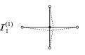
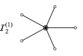
Figure 2: One loop five-point parity even and odd amplitude graphs. This is just a one loop box in dual coordinates, and a pentagon graph. The starred vertex $v$ indicates a factor $i\epsilon_{12345v}$.

In section 7 we show that this form of the five-point amplitude integrand is consistent with both the local expression in terms of twistors [28], and with the all orders in $\epsilon$ version containing a parity odd pentagon at order $\epsilon$, [56].

4 Two loops

We now proceed to investigate $M_{5}^{(2)}$. The refined duality equation (26) gives two equations involving $M_{5}^{(2)}$ and lower loop amplitudes, namely for $\ell=2,m=0$ and for $\ell=3,m=1$

$${F^{(2)}_{5;0}}\ =\ M_{5}^{(2)}+\overline{M}_{5}^{(2)}$$ (41)

$${F^{(3)}_{5;1}}\ =\ M_{5}^{(2)}\overline{M}_{5}^{(1)}+M_{5}^{(1)}\overline{M}_{5}^{(2)}\ .$$ (42)

Therefore as before, since we have two equations for two unknowns, $M_{5}^{(2)}$ and $\overline{M}_{5}^{(2)}$, we can solve for these.

To do this first rewrite the equations as:

$$M_{5}^{(2)}+\overline{M}_{5}^{(2)}\ =\ {F^{(2)}_{5;0}}$$ (43)

$$\left(M_{5}^{(2)}-\overline{M}_{5}^{(2)}\right)\left(M_{5}^{(1)}-\overline{M}_{5}^{(1)}\right) =F^{(2)}_{5;0}F^{(1)}-2F^{(3)}_{5;1}\ ,$$ (44)

thus giving an equation for the parity odd part of the two loop amplitude in term of correlator quantities $F$’s and the one loop parity odd amplitude.

Once more we can simplify the parity odd part of the amplitude at two loops. To do this, we write an ansatz for the form of $M_{5}^{(2)}-\overline{M}_{5}^{(2)}$. Since it is parity odd it must contain one factor of the six-dimensional $\epsilon$ tensor. By examination we find the parity odd part of the two loop amplitude is

$${M_{5}^{(2)}-\overline{M}_{5}^{(2)}}={1\over 2!}\text{cyc}\left({\pm i\epsilon_{123456}x^{2}_{35}\over x^{2}_{16}x^{2}_{26}x^{2}_{36}x^{2}_{56}x^{2}_{37}x^{2}_{47}x^{2}_{57}x^{2}_{67}}\right)$$ (45)

which is a pentabox with an epsilon in the numerator. Note that the $\pm$ here is the same as the 1 loop one, so once that sign is fixed so will this two loop one.

The full two-loop amplitude is then

$$M^{(2)}_{5}=\frac{1}{2\times 2!}\left({\cal I}_{1}^{(2)}+{\cal I}_{2}^{(2)}+{\cal I}_{3}^{(2)}\right)$$ (46)

where

$$\mathcal{I}_{1}^{(2)} =\text{cyc}\left[\frac{x_{13}^{4}x_{25}^{2}}{x_{16}^{2}x_{17}^{2}x_{27}^{2}x_{36}^{2}x_{37}^{2}x_{56}^{2}x_{67}^{2}}\right] \mathcal{I}_{2}^{(2)} =\text{cyc}\left[\frac{x_{16}^{2}x_{24}^{2}x_{25}^{2}x_{35}^{2}}{x_{17}^{2}x_{26}^{2}x_{27}^{2}x_{36}^{2}x_{46}^{2}x_{56}^{2}x_{57}^{2}x_{67}^{2}}\right]$$ (47)

$$\mathcal{I}_{3}^{(2)} =\text{cyc}\left[\frac{ix_{13}^{2}\epsilon_{123456}}{x_{16}^{2}x_{17}^{2}x_{27}^{2}x_{36}^{2}x_{37}^{2}x_{46}^{2}x_{56}^{2}x_{67}^{2}}\right]$$

with corresponding graphs

 

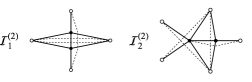
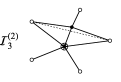
Figure 3: Two loop five-point parity even (${\cal I}_{1}^{(2)}$ and ${\cal I}_{2}^{(2)}$) and parity odd (${\cal I}_{3}^{(2)}$) amplitude graphs. The starred vertex $v$ indicates a factor $i\,\epsilon_{12345v}$.

5 Higher loops

This process can clearly be extended to higher orders. At $\ell$-loops we use the refined duality (26) with $\ell,m=0$ and $\ell+1,m=1$ giving

$${F^{(\ell)}_{5;0}}\ =\ M_{5}^{(\ell)}+\overline{M}_{5}^{(\ell)}$$ (48)

$${F^{(\ell+1)}_{5;1}}\ =\ M_{5}^{(\ell)}\overline{M}_{5}^{(1)}+M_{5}^{(1)}\overline{M}_{5}^{(\ell)}\ .$$ (49)

From (48) we can immediately read off the parity even part $M_{5}^{(\ell)}+\overline{M}_{5}^{(\ell)}$. Then similarly to (44) we can write

$$\left(M_{5}^{(\ell)}-\overline{M}_{5}^{(\ell)}\right)\left(M_{5}^{(1)}-\overline{M}_{5}^{(1)}\right) =F^{(\ell)}_{5;0}F^{(1)}-2F^{(\ell+1)}_{5;1}\ ,$$ (50)

giving the parity odd part of the $\ell$ loop graph in terms of correlator quantities ($F$’s) and the one-loop amplitude. So knowing the right-hand side of this equation we can compute the parity odd combination $M_{5}^{\ell}-\bar{M}_{5}^{(\ell)}$.

Now as at two loops we wish to rewrite this in a simpler form, i.e. in terms of $\epsilon_{123456}$. In principle we could include epsilon objects with two or more internal variables so for example $\epsilon_{123467}$. However we have always found solutions in which only a single internal variable appears in the $\epsilon$. We therefore make the following assumption:

Assumption: The parity odd part of the five-point amplitude at any loop can always be written in the form $\int d^{4}x_{6}\dots d^{4}x_{5+\ell}\,\epsilon_{123456}\,f(x_{i})$ where $f(x_{i})$ is an integrand composed of $x_{ij}^{2}$ depending on all external and internal variables. There never is an epsilon tensor involving two or more internal points.

With the help of this it is remarkably straightforward to compute the parity odd part of the amplitude at $\ell$ loops from the correlator. In the combination $\left(M_{5}^{(\ell)}-\overline{M}_{5}^{(\ell)}\right)\left(M_{5}^{(1)}-\overline{M}_{5}^{(1)}\right)$ on the l.h.s. of (50) we have to consider the product of two epsilon tensors, one from $\ell$ loops using the above conjecture and one from one loop. This product contains a single term involving an inverse propagator between two internal vertices (see (38))

$$\epsilon_{123456}\,\epsilon_{123457}\,=\,2\,{\bf x_{67}^{2}}\,x_{13}^{2}x_{35}^{2}x_{25}^{2}x_{24}^{2}x_{14}^{2}+\dots\ .$$ (51)

Thus this will produce a product graph, a pentagon around $x_{6}$ glued to a higher loop graph involving $x_{7}$ together with a numerator $x_{67}^{2}$ between them. Such a product graph with numerator can be produced from the correlator $F^{(\ell+1)}_{5;1}$ but can not be cancelled by any terms on the right hand side of (50). Thus each graph of this type in $F^{(\ell+1)}_{5;1}$ uniquely singles out a corresponding $\epsilon$-term in $M_{5}^{(\ell)}-\overline{M}_{5}^{(\ell)}$.

This can again be interpreted in terms of correlator $f$-graphs: 5-cycles in the $f$-graph split the graph into two halves. We look for 5-cycles which have the 1 loop pentagon graph on one side. The other side then gives us the parity odd graph in question. Its coefficient is inherited from the $f$-graph. The procedure is illustrated in Figure 4.

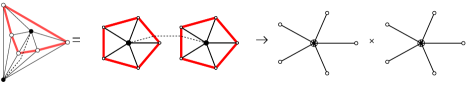
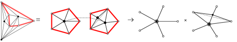
Figure 4: Figure illustrating the procedure for obtaining the parity odd part of the five-point amplitude from the correlator $f$-graphs. The 5-cycle (shown in thick red) splits the graph into two parts. The inside of the 5-cycle corresponds to the 1 loop parity odd pentagon, whereas the outside corresponds to the higher loop parity odd graph. The starred vertex is the vertex attached to the 1 loop internal vertex via an internal line. In the first line we start with a 5-cycle in $f^{(3)}$ contributing to $F_{1}^{(2)}$, the “outside” of which determines the parity odd graph for $M_{5}^{(1)}$. In the second line we start with a 5-cycle in one of the three $f$-graphs contributing to $f^{(4)}$ contributing to $F_{5}^{(2)}$ thus giving a contribution to $F^{(3)}_{5;1}$. The “outside” of the 5-cycle then determines the parity odd graph for $M_{5}^{(2)}$.

That this simple rule then correctly reproduces the entire right-hand side of (50) appears somewhat miraculous and relies on many cancellations between graphs. We will attempt to give some motivation of why/how this works in the conclusions. Notice that this consistency determines many of the correlator coefficients not determined from the four-point duality (determined by the rung rule which arises from consistency of the four-point amplitude/correlator duality). The first coefficient not determined by five-point consistency appears in $f^{(6)}$.

Note there are of course further consistency requirements on this picture, starting at four loops, since we require the $m=2$ part of $F_{5}^{(4)}$ to be given by the product of two loop amplitudes (which were determined by $F^{(2)}_{5;0}$ and $F^{(3)}_{5;1}$ i.e. $F^{(4)}_{5;2}=M_{5}^{(2)}\bar{M}_{5}^{(2)}$.

Using this method we have obtained the full the three-loop five-point amplitude (parity even and parity odd part) and checked that it indeed satisfies the consistency condition (50):

$$M_{5}^{(3)}={1\over 2}{1\over 3!}\int d^{4}x_{6}d^{4}x_{7}d^{4}x_{8}\left(\sum_{i=1}^{13}c_{i}{\cal I}_{i}^{(3)}\right)\,,$$ (52)

where

$$c_{1}=\dots=c_{6}=c_{9}=\dots c_{12}=1\,,\qquad c_{7}=c_{8}=c_{13}=-1.$$ (53)

and

$$\mathcal{I}_{1}^{(3)} =\text{cyc}\left(\frac{x_{13}^{6}x_{25}^{2}}{x_{16}^{2}x_{17}^{2}x_{18}^{2}x_{28}^{2}x_{36}^{2}x_{37}^{2}x_{38}^{2}x_{57}^{2}x_{67}^{2}x_{68}^{2}}\right) \mathcal{I}_{2}^{(3)} =\text{cyc}\left(\frac{x_{16}^{4}x_{24}^{2}x_{25}^{2}x_{35}^{2}}{x_{17}^{2}x_{18}^{2}x_{26}^{2}x_{28}^{2}x_{36}^{2}x_{46}^{2}x_{56}^{2}x_{57}^{2}x_{67}^{2}x_{68}^{2}x_{78}^{2}}\right)$$ (54)

$$\mathcal{I}_{3}^{(3)} =\text{cyc}\left(\frac{x_{13}^{4}x_{25}^{2}x_{35}^{2}x_{46}^{2}}{x_{16}^{2}x_{18}^{2}x_{28}^{2}x_{36}^{2}x_{37}^{2}x_{38}^{2}x_{47}^{2}x_{56}^{2}x_{57}^{2}x_{67}^{2}x_{68}^{2}}\right) \mathcal{I}_{4}^{(3)} =\text{cyc}\left(\frac{x_{13}^{4}x_{24}^{2}x_{46}^{2}}{x_{16}^{2}x_{18}^{2}x_{26}^{2}x_{36}^{2}x_{37}^{2}x_{47}^{2}x_{48}^{2}x_{67}^{2}x_{68}^{2}x_{78}^{2}}\right)$$

$$\mathcal{I}_{5}^{(3)} =\text{cyc}\left(\frac{x_{14}^{2}x_{16}^{2}x_{24}^{2}x_{25}^{2}x_{37}^{2}}{x_{17}^{2}x_{18}^{2}x_{26}^{2}x_{28}^{2}x_{36}^{2}x_{46}^{2}x_{47}^{2}x_{57}^{2}x_{67}^{2}x_{68}^{2}x_{78}^{2}}\right) \mathcal{I}_{6}^{(3)} =\text{cyc}\left(\frac{x_{16}^{2}x_{24}^{2}x_{25}^{4}x_{35}^{2}}{x_{18}^{2}x_{26}^{2}x_{27}^{2}x_{28}^{2}x_{36}^{2}x_{46}^{2}x_{56}^{2}x_{57}^{2}x_{58}^{2}x_{67}^{2}x_{78}^{2}}\right)$$

$$\mathcal{I}_{7}^{(3)} =\text{cyc}\left(\frac{x_{13}^{2}x_{24}^{2}x_{25}^{2}x_{35}^{2}}{x_{18}^{2}x_{26}^{2}x_{28}^{2}x_{36}^{2}x_{37}^{2}x_{47}^{2}x_{57}^{2}x_{58}^{2}x_{67}^{2}x_{68}^{2}}\right) \mathcal{I}_{8}^{(3)} =\text{cyc}\left(\frac{x_{13}^{2}x_{14}^{2}x_{35}^{2}}{x_{16}^{2}x_{17}^{2}x_{36}^{2}x_{38}^{2}x_{48}^{2}x_{57}^{2}x_{67}^{2}x_{68}^{2}x_{78}^{2}}\right)$$

$$\mathcal{I}_{9}^{(3)} =\text{cyc}\left(\frac{ix_{13}^{4}\epsilon_{123456}}{x_{16}^{2}x_{17}^{2}x_{18}^{2}x_{28}^{2}x_{36}^{2}x_{37}^{2}x_{38}^{2}x_{46}^{2}x_{56}^{2}x_{67}^{2}x_{78}^{2}}\right) \mathcal{I}_{10}^{(3)} =\text{cyc}\left(\frac{ix_{13}^{2}x_{14}^{2}\epsilon_{123456}}{x_{16}^{2}x_{17}^{2}x_{18}^{2}x_{28}^{2}x_{36}^{2}x_{38}^{2}x_{46}^{2}x_{47}^{2}x_{57}^{2}x_{67}^{2}x_{68}^{2}}\right)$$

$$\mathcal{I}_{11}^{(3)} =\text{cyc}\left(\frac{ix_{24}^{2}x_{36}^{2}\epsilon_{123456}}{x_{16}^{2}x_{26}^{2}x_{28}^{2}x_{37}^{2}x_{38}^{2}x_{46}^{2}x_{47}^{2}x_{56}^{2}x_{67}^{2}x_{68}^{2}x_{78}^{2}}\right) \mathcal{I}_{12}^{(3)} =\text{cyc}\left(\frac{ix_{14}^{2}x_{27}^{2}\epsilon_{123456}}{x_{17}^{2}x_{18}^{2}x_{26}^{2}x_{28}^{2}x_{36}^{2}x_{46}^{2}x_{47}^{2}x_{57}^{2}x_{67}^{2}x_{68}^{2}x_{78}^{2}}\right)$$

$$\mathcal{I}_{13}^{(3)} =\text{cyc}\left(\frac{ix_{13}^{2}\epsilon_{123456}}{x_{16}^{2}x_{17}^{2}x_{26}^{2}x_{36}^{2}x_{38}^{2}x_{48}^{2}x_{57}^{2}x_{67}^{2}x_{68}^{2}x_{78}^{2}}\right)$$

also illustrated graphically in figures 5 and 6

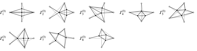
Figure 5: Three loop five-point parity even amplitude graphs. White vertices indicate external points, $x_{1},x_{2},x_{3},x_{4},x_{5}$ which are cyclically ordered in either orientation and black nodes integration variables $x_{6},x_{7},x_{8}$. A black line between vertices $i$ and $j$ indicates a propagator term $1/x_{ij}^{2}$. A dotted line indicates an inverse propagator $x_{ij}^{2}$. The integrand expression ${\cal I}_{i}^{(3)}$ is the expression thus obtained by summing over all different such labellings.

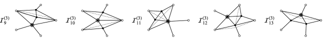
Figure 6: Three loop five-point parity odd amplitude graphs. A starred vertex $v$ indicates a factor $i\epsilon_{12345v}$.

6 Four- and five-loops amplitude

Similarly, using the method outlined in the previous section we have obtained the full (parity even and parity odd part) four-loop five-point amplitude and checked that it satisfies the consistency condition (50). For the four-loop result:

$$M_{5}^{(4)}={1\over 2}{1\over 4!}\int d^{4}x_{6}d^{4}x_{7}d^{4}x_{8}d^{4}x_{9}\left(\sum_{i=1}^{71}c_{i}{\cal I}_{i}^{(4)}\right)\,,$$ (55)

where

$$c_{1}=\dots=c_{28}=c_{45}=\dots=c_{62}=1\,,$$ (56)

$$c_{29}=\dots=c_{44}=c_{63}=\dots=c_{71}=-1\$$

and

$$\mathcal{I}_{1}^{(4)} =\text{cyc}\left[\frac{x_{13}^{8}x_{25}^{2}}{x_{16}^{2}x_{17}^{2}x_{18}^{2}x_{19}^{2}x_{29}^{2}x_{36}^{2}x_{37}^{2}x_{38}^{2}x_{39}^{2}x_{57}^{2}x_{68}^{2}x_{69}^{2}x_{78}^{2}}\right] \mathcal{I}_{2}^{(4)} =\text{cyc}\left[\frac{x_{16}^{6}x_{24}^{2}x_{25}^{2}x_{35}^{2}}{x_{17}^{2}x_{18}^{2}x_{19}^{2}x_{26}^{2}x_{29}^{2}x_{36}^{2}x_{46}^{2}x_{56}^{2}x_{58}^{2}x_{67}^{2}x_{68}^{2}x_{69}^{2}x_{78}^{2}x_{79}^{2}}\right]$$

$$\mathcal{I}_{3}^{(4)} =\text{cyc}\left[\frac{x_{13}^{2}x_{24}^{2}x_{25}^{2}x_{35}^{2}}{x_{19}^{2}x_{28}^{2}x_{29}^{2}x_{37}^{2}x_{38}^{2}x_{47}^{2}x_{56}^{2}x_{59}^{2}x_{67}^{2}x_{68}^{2}x_{69}^{2}x_{78}^{2}}\right] \mathcal{I}_{4}^{(4)} =\text{cyc}\left[\frac{x_{14}^{2}x_{24}^{2}x_{25}^{2}}{x_{17}^{2}x_{26}^{2}x_{29}^{2}x_{48}^{2}x_{49}^{2}x_{57}^{2}x_{67}^{2}x_{68}^{2}x_{69}^{2}x_{78}^{2}x_{89}^{2}}\right]$$

$$\mathcal{I}_{5}^{(4)} =\text{cyc}\left[\frac{x_{13}^{6}x_{25}^{2}x_{35}^{2}x_{46}^{2}}{x_{16}^{2}x_{17}^{2}x_{19}^{2}x_{29}^{2}x_{36}^{2}x_{37}^{2}x_{38}^{2}x_{39}^{2}x_{48}^{2}x_{56}^{2}x_{58}^{2}x_{67}^{2}x_{68}^{2}x_{79}^{2}}\right] \mathcal{I}_{6}^{(4)} =\text{cyc}\left[\frac{x_{13}^{6}x_{24}^{2}x_{67}^{2}}{x_{16}^{2}x_{17}^{2}x_{19}^{2}x_{26}^{2}x_{36}^{2}x_{37}^{2}x_{38}^{2}x_{47}^{2}x_{68}^{2}x_{69}^{2}x_{78}^{2}x_{79}^{2}x_{89}^{2}}\right]$$

$$\mathcal{I}_{7}^{(4)} =\text{cyc}\left[\frac{x_{14}^{6}x_{35}^{2}x_{36}^{2}}{x_{16}^{2}x_{17}^{2}x_{19}^{2}x_{38}^{2}x_{39}^{2}x_{46}^{2}x_{47}^{2}x_{48}^{2}x_{57}^{2}x_{67}^{2}x_{68}^{2}x_{69}^{2}x_{89}^{2}}\right] \mathcal{I}_{8}^{(4)} =\text{cyc}\left[\frac{x_{14}^{2}x_{16}^{4}x_{24}^{2}x_{25}^{2}x_{37}^{2}}{x_{17}^{2}x_{18}^{2}x_{19}^{2}x_{26}^{2}x_{29}^{2}x_{36}^{2}x_{46}^{2}x_{47}^{2}x_{57}^{2}x_{67}^{2}x_{68}^{2}x_{69}^{2}x_{78}^{2}x_{89}^{2}}\right]$$

$$\mathcal{I}_{9}^{(4)} =\text{cyc}\left[\frac{x_{16}^{4}x_{24}^{2}x_{25}^{2}x_{35}^{4}}{x_{17}^{2}x_{19}^{2}x_{26}^{2}x_{29}^{2}x_{36}^{2}x_{38}^{2}x_{48}^{2}x_{56}^{2}x_{57}^{2}x_{58}^{2}x_{67}^{2}x_{68}^{2}x_{69}^{2}x_{79}^{2}}\right] \mathcal{I}_{10}^{(4)} =\text{cyc}\left[\frac{x_{16}^{4}x_{24}^{2}x_{25}^{2}x_{35}^{2}x_{57}^{2}}{x_{17}^{2}x_{19}^{2}x_{26}^{2}x_{27}^{2}x_{36}^{2}x_{46}^{2}x_{56}^{2}x_{58}^{2}x_{59}^{2}x_{67}^{2}x_{68}^{2}x_{78}^{2}x_{79}^{2}x_{89}^{2}}\right]$$

$$\mathcal{I}_{11}^{(4)} =\text{cyc}\left[\frac{x_{13}^{6}x_{14}^{2}x_{27}^{2}x_{35}^{2}}{x_{16}^{2}x_{17}^{2}x_{18}^{2}x_{19}^{2}x_{26}^{2}x_{36}^{2}x_{37}^{2}x_{38}^{2}x_{39}^{2}x_{47}^{2}x_{57}^{2}x_{69}^{2}x_{78}^{2}x_{89}^{2}}\right] \mathcal{I}_{12}^{(4)} =\text{cyc}\left[\frac{x_{13}^{2}x_{17}^{4}x_{24}^{4}}{x_{16}^{2}x_{18}^{2}x_{19}^{2}x_{26}^{2}x_{27}^{2}x_{37}^{2}x_{47}^{2}x_{48}^{2}x_{67}^{2}x_{69}^{2}x_{78}^{2}x_{79}^{2}x_{89}^{2}}\right]$$

$$\mathcal{I}_{13}^{(4)} =\text{cyc}\left[\frac{x_{16}^{4}x_{24}^{2}x_{25}^{2}x_{35}^{2}x_{37}^{2}}{x_{17}^{2}x_{18}^{2}x_{27}^{2}x_{29}^{2}x_{36}^{2}x_{39}^{2}x_{46}^{2}x_{56}^{2}x_{58}^{2}x_{67}^{2}x_{68}^{2}x_{69}^{2}x_{78}^{2}x_{79}^{2}}\right] \mathcal{I}_{14}^{(4)} =\text{cyc}\left[\frac{x_{13}^{4}x_{17}^{2}x_{25}^{2}x_{35}^{2}x_{46}^{2}}{x_{16}^{2}x_{18}^{2}x_{19}^{2}x_{29}^{2}x_{36}^{2}x_{37}^{2}x_{39}^{2}x_{47}^{2}x_{57}^{2}x_{58}^{2}x_{67}^{2}x_{68}^{2}x_{69}^{2}x_{78}^{2}}\right]$$

$$\mathcal{I}_{15}^{(4)} =\text{cyc}\left[\frac{x_{13}^{4}x_{17}^{2}x_{24}^{2}x_{46}^{2}}{x_{16}^{2}x_{18}^{2}x_{19}^{2}x_{26}^{2}x_{36}^{2}x_{37}^{2}x_{47}^{2}x_{48}^{2}x_{67}^{2}x_{69}^{2}x_{78}^{2}x_{79}^{2}x_{89}^{2}}\right] \mathcal{I}_{16}^{(4)} =\text{cyc}\left[\frac{x_{13}^{4}x_{14}^{4}x_{24}^{2}x_{56}^{2}}{x_{16}^{2}x_{17}^{2}x_{18}^{2}x_{19}^{2}x_{29}^{2}x_{36}^{2}x_{39}^{2}x_{46}^{2}x_{47}^{2}x_{48}^{2}x_{58}^{2}x_{67}^{2}x_{69}^{2}x_{78}^{2}}\right]$$

$$\mathcal{I}_{17}^{(4)} =\text{cyc}\left[\frac{x_{16}^{2}x_{18}^{2}x_{24}^{2}x_{25}^{2}x_{35}^{2}x_{37}^{2}}{x_{17}^{2}x_{19}^{2}x_{26}^{2}x_{29}^{2}x_{36}^{2}x_{38}^{2}x_{48}^{2}x_{57}^{2}x_{58}^{2}x_{67}^{2}x_{68}^{2}x_{69}^{2}x_{78}^{2}x_{79}^{2}}\right] \mathcal{I}_{18}^{(4)} =\text{cyc}\left[\frac{x_{16}^{2}x_{17}^{2}x_{24}^{2}x_{25}^{4}x_{35}^{2}}{x_{18}^{2}x_{19}^{2}x_{26}^{2}x_{27}^{2}x_{29}^{2}x_{36}^{2}x_{46}^{2}x_{56}^{2}x_{57}^{2}x_{58}^{2}x_{67}^{2}x_{78}^{2}x_{79}^{2}x_{89}^{2}}\right]$$

$$\mathcal{I}_{19}^{(4)} =\text{cyc}\left[\frac{x_{13}^{2}x_{14}^{2}x_{26}^{2}x_{35}^{4}x_{46}^{2}}{x_{16}^{2}x_{19}^{2}x_{29}^{2}x_{36}^{2}x_{37}^{2}x_{39}^{2}x_{47}^{2}x_{48}^{2}x_{56}^{2}x_{58}^{2}x_{67}^{2}x_{68}^{2}x_{69}^{2}x_{78}^{2}}\right] \mathcal{I}_{20}^{(4)} =\text{cyc}\left[\frac{x_{13}^{2}x_{14}^{2}x_{26}^{2}x_{35}^{2}x_{36}^{2}x_{47}^{2}}{x_{16}^{2}x_{17}^{2}x_{27}^{2}x_{37}^{2}x_{38}^{2}x_{39}^{2}x_{46}^{2}x_{48}^{2}x_{56}^{2}x_{67}^{2}x_{68}^{2}x_{69}^{2}x_{79}^{2}x_{89}^{2}}\right]$$

$$\mathcal{I}_{21}^{(4)} =\text{cyc}\left[\frac{x_{13}^{2}x_{14}^{2}x_{24}^{2}x_{26}^{2}x_{36}^{2}x_{57}^{2}}{x_{16}^{2}x_{19}^{2}x_{27}^{2}x_{29}^{2}x_{37}^{2}x_{38}^{2}x_{46}^{2}x_{48}^{2}x_{56}^{2}x_{67}^{2}x_{68}^{2}x_{69}^{2}x_{78}^{2}x_{79}^{2}}\right] \mathcal{I}_{22}^{(4)} =\text{cyc}\left[\frac{x_{14}^{2}x_{24}^{4}x_{25}^{2}x_{36}^{2}x_{67}^{2}}{x_{16}^{2}x_{26}^{2}x_{27}^{2}x_{29}^{2}x_{37}^{2}x_{46}^{2}x_{47}^{2}x_{48}^{2}x_{56}^{2}x_{68}^{2}x_{69}^{2}x_{78}^{2}x_{79}^{2}x_{89}^{2}}\right]$$

$$\mathcal{I}_{23}^{(4)} =\text{cyc}\left[\frac{x_{17}^{2}x_{24}^{2}x_{25}^{4}x_{35}^{2}x_{36}^{2}}{x_{19}^{2}x_{26}^{2}x_{28}^{2}x_{29}^{2}x_{37}^{2}x_{38}^{2}x_{47}^{2}x_{56}^{2}x_{57}^{2}x_{59}^{2}x_{67}^{2}x_{68}^{2}x_{69}^{2}x_{78}^{2}}\right] \mathcal{I}_{24}^{(4)} =\text{cyc}\left[\frac{x_{14}^{4}x_{24}^{2}x_{25}^{2}x_{27}^{2}x_{36}^{2}}{x_{17}^{2}x_{19}^{2}x_{26}^{2}x_{28}^{2}x_{29}^{2}x_{38}^{2}x_{46}^{2}x_{47}^{2}x_{48}^{2}x_{57}^{2}x_{67}^{2}x_{68}^{2}x_{69}^{2}x_{79}^{2}}\right]$$

$$\mathcal{I}_{25}^{(4)} =\text{cyc}\left[\frac{x_{13}^{2}x_{18}^{2}x_{24}^{4}x_{36}^{2}}{x_{16}^{2}x_{17}^{2}x_{26}^{2}x_{29}^{2}x_{38}^{2}x_{39}^{2}x_{47}^{2}x_{48}^{2}x_{67}^{2}x_{68}^{2}x_{69}^{2}x_{78}^{2}x_{89}^{2}}\right] \mathcal{I}_{26}^{(4)} =\text{cyc}\left[\frac{x_{13}^{2}x_{18}^{2}x_{25}^{2}x_{27}^{2}x_{35}^{2}x_{46}^{2}}{x_{17}^{2}x_{19}^{2}x_{26}^{2}x_{29}^{2}x_{36}^{2}x_{38}^{2}x_{48}^{2}x_{57}^{2}x_{58}^{2}x_{67}^{2}x_{68}^{2}x_{69}^{2}x_{78}^{2}x_{79}^{2}}\right]$$

$$\mathcal{I}_{27}^{(4)} =\text{cyc}\left[\frac{x_{13}^{2}x_{14}^{2}x_{19}^{2}x_{28}^{2}x_{35}^{2}x_{46}^{2}}{x_{16}^{2}x_{17}^{2}x_{18}^{2}x_{26}^{2}x_{36}^{2}x_{39}^{2}x_{48}^{2}x_{49}^{2}x_{58}^{2}x_{67}^{2}x_{69}^{2}x_{78}^{2}x_{79}^{2}x_{89}^{2}}\right] \mathcal{I}_{28}^{(4)} =\text{cyc}\left[\frac{x_{18}^{2}x_{24}^{4}x_{25}^{2}x_{35}^{2}x_{67}^{2}}{x_{16}^{2}x_{26}^{2}x_{27}^{2}x_{29}^{2}x_{37}^{2}x_{47}^{2}x_{48}^{2}x_{56}^{2}x_{58}^{2}x_{68}^{2}x_{69}^{2}x_{78}^{2}x_{79}^{2}x_{89}^{2}}\right]$$

$$\mathcal{I}_{29}^{(4)} =\text{cyc}\left[\frac{x_{13}^{4}x_{25}^{2}x_{35}^{2}}{x_{18}^{2}x_{19}^{2}x_{29}^{2}x_{36}^{2}x_{37}^{2}x_{39}^{2}x_{57}^{2}x_{58}^{2}x_{67}^{2}x_{68}^{2}x_{69}^{2}x_{78}^{2}}\right] \mathcal{I}_{30}^{(4)} =\text{cyc}\left[\frac{x_{14}^{4}x_{35}^{2}}{x_{18}^{2}x_{19}^{2}x_{39}^{2}x_{46}^{2}x_{47}^{2}x_{56}^{2}x_{67}^{2}x_{68}^{2}x_{78}^{2}x_{79}^{2}x_{89}^{2}}\right]$$

$$\mathcal{I}_{31}^{(4)} =\text{cyc}\left[\frac{x_{16}^{2}x_{24}^{2}x_{25}^{2}x_{35}^{2}}{x_{19}^{2}x_{26}^{2}x_{29}^{2}x_{36}^{2}x_{48}^{2}x_{57}^{2}x_{58}^{2}x_{67}^{2}x_{68}^{2}x_{69}^{2}x_{78}^{2}x_{79}^{2}}\right] \mathcal{I}_{32}^{(4)} =\text{cyc}\left[\frac{x_{14}^{2}x_{16}^{2}x_{24}^{2}x_{25}^{2}x_{35}^{2}}{x_{17}^{2}x_{19}^{2}x_{26}^{2}x_{27}^{2}x_{36}^{2}x_{46}^{2}x_{48}^{2}x_{58}^{2}x_{59}^{2}x_{67}^{2}x_{68}^{2}x_{79}^{2}x_{89}^{2}}\right]$$

$$\mathcal{I}_{33}^{(4)} =\text{cyc}\left[\frac{x_{13}^{4}x_{14}^{2}x_{24}^{2}x_{35}^{2}}{x_{16}^{2}x_{18}^{2}x_{19}^{2}x_{26}^{2}x_{36}^{2}x_{37}^{2}x_{39}^{2}x_{47}^{2}x_{48}^{2}x_{58}^{2}x_{69}^{2}x_{78}^{2}x_{79}^{2}}\right] \mathcal{I}_{34}^{(4)} =\text{cyc}\left[\frac{x_{14}^{2}x_{17}^{2}x_{24}^{2}x_{25}^{2}}{x_{16}^{2}x_{19}^{2}x_{26}^{2}x_{27}^{2}x_{47}^{2}x_{48}^{2}x_{58}^{2}x_{67}^{2}x_{69}^{2}x_{78}^{2}x_{79}^{2}x_{89}^{2}}\right]$$

$$\mathcal{I}_{35}^{(4)} =\text{cyc}\left[\frac{x_{13}^{2}x_{14}^{2}x_{17}^{2}x_{35}^{2}}{x_{16}^{2}x_{18}^{2}x_{19}^{2}x_{37}^{2}x_{39}^{2}x_{47}^{2}x_{58}^{2}x_{67}^{2}x_{68}^{2}x_{69}^{2}x_{78}^{2}x_{79}^{2}}\right] \mathcal{I}_{36}^{(4)} =\text{cyc}\left[\frac{x_{13}^{2}x_{14}^{2}x_{17}^{2}x_{25}^{2}x_{35}^{2}}{x_{16}^{2}x_{18}^{2}x_{19}^{2}x_{29}^{2}x_{37}^{2}x_{39}^{2}x_{47}^{2}x_{56}^{2}x_{57}^{2}x_{67}^{2}x_{68}^{2}x_{78}^{2}x_{89}^{2}}\right]$$

$$\mathcal{I}_{37}^{(4)} =\text{cyc}\left[\frac{x_{16}^{2}x_{24}^{2}x_{25}^{2}x_{35}^{2}}{x_{19}^{2}x_{28}^{2}x_{29}^{2}x_{36}^{2}x_{46}^{2}x_{56}^{2}x_{57}^{2}x_{67}^{2}x_{68}^{2}x_{78}^{2}x_{79}^{2}x_{89}^{2}}\right] \mathcal{I}_{38}^{(4)} =\text{cyc}\left[\frac{x_{14}^{2}x_{17}^{2}x_{24}^{2}x_{25}^{2}x_{35}^{2}}{x_{16}^{2}x_{18}^{2}x_{28}^{2}x_{29}^{2}x_{39}^{2}x_{47}^{2}x_{49}^{2}x_{56}^{2}x_{57}^{2}x_{67}^{2}x_{68}^{2}x_{78}^{2}x_{79}^{2}}\right]$$

$$\mathcal{I}_{39}^{(4)} =\text{cyc}\left[\frac{x_{13}^{4}x_{25}^{4}}{x_{16}^{2}x_{19}^{2}x_{27}^{2}x_{29}^{2}x_{37}^{2}x_{38}^{2}x_{56}^{2}x_{58}^{2}x_{68}^{2}x_{69}^{2}x_{78}^{2}x_{79}^{2}}\right] \mathcal{I}_{40}^{(4)} =\text{cyc}\left[\frac{x_{13}^{4}x_{14}^{2}x_{27}^{2}x_{35}^{2}}{x_{16}^{2}x_{17}^{2}x_{18}^{2}x_{26}^{2}x_{36}^{2}x_{37}^{2}x_{39}^{2}x_{49}^{2}x_{58}^{2}x_{67}^{2}x_{78}^{2}x_{79}^{2}x_{89}^{2}}\right]$$

$$\mathcal{I}_{41}^{(4)} =\text{cyc}\left[\frac{x_{16}^{2}x_{24}^{4}x_{25}^{2}x_{35}^{2}}{x_{19}^{2}x_{26}^{2}x_{27}^{2}x_{29}^{2}x_{36}^{2}x_{46}^{2}x_{48}^{2}x_{58}^{2}x_{59}^{2}x_{67}^{2}x_{68}^{2}x_{78}^{2}x_{79}^{2}}\right] \mathcal{I}_{42}^{(4)} =\text{cyc}\left[\frac{x_{13}^{2}x_{16}^{2}x_{25}^{2}x_{28}^{2}x_{35}^{2}}{x_{17}^{2}x_{18}^{2}x_{26}^{2}x_{27}^{2}x_{36}^{2}x_{39}^{2}x_{58}^{2}x_{59}^{2}x_{67}^{2}x_{68}^{2}x_{69}^{2}x_{78}^{2}x_{89}^{2}}\right]$$

$$\mathcal{I}_{43}^{(4)} =\text{cyc}\left[\frac{x_{14}^{2}x_{16}^{2}x_{24}^{2}x_{25}^{2}x_{37}^{2}}{x_{17}^{2}x_{18}^{2}x_{26}^{2}x_{27}^{2}x_{36}^{2}x_{46}^{2}x_{49}^{2}x_{58}^{2}x_{67}^{2}x_{69}^{2}x_{78}^{2}x_{79}^{2}x_{89}^{2}}\right] \mathcal{I}_{44}^{(4)} =\text{cyc}\left[\frac{x_{13}^{2}x_{14}^{2}x_{17}^{2}x_{24}^{2}x_{35}^{2}x_{69}^{2}}{x_{16}^{2}x_{18}^{2}x_{19}^{2}x_{29}^{2}x_{37}^{2}x_{39}^{2}x_{46}^{2}x_{47}^{2}x_{56}^{2}x_{67}^{2}x_{68}^{2}x_{78}^{2}x_{79}^{2}x_{89}^{2}}\right]$$

$$\mathcal{I}_{45}^{(4)} =\text{cyc}\left[\frac{ix_{13}^{6}\epsilon_{123456}}{x_{16}^{2}x_{17}^{2}x_{18}^{2}x_{19}^{2}x_{29}^{2}x_{36}^{2}x_{37}^{2}x_{38}^{2}x_{39}^{2}x_{46}^{2}x_{56}^{2}x_{68}^{2}x_{78}^{2}x_{79}^{2}}\right] \mathcal{I}_{46}^{(4)} =\text{cyc}\left[\frac{ix_{13}^{2}\epsilon_{123456}}{x_{16}^{2}x_{19}^{2}x_{26}^{2}x_{36}^{2}x_{38}^{2}x_{47}^{2}x_{57}^{2}x_{68}^{2}x_{69}^{2}x_{78}^{2}x_{79}^{2}x_{89}^{2}}\right]$$

$$\mathcal{I}_{47}^{(4)} =\text{cyc}\left[\frac{ix_{13}^{4}x_{14}^{2}\epsilon_{123456}}{x_{16}^{2}x_{17}^{2}x_{18}^{2}x_{19}^{2}x_{29}^{2}x_{36}^{2}x_{37}^{2}x_{39}^{2}x_{46}^{2}x_{48}^{2}x_{58}^{2}x_{67}^{2}x_{68}^{2}x_{79}^{2}}\right] \mathcal{I}_{48}^{(4)} =\text{cyc}\left[\frac{ix_{16}^{4}x_{25}^{2}\epsilon_{123456}}{x_{17}^{2}x_{18}^{2}x_{19}^{2}x_{26}^{2}x_{27}^{2}x_{36}^{2}x_{46}^{2}x_{56}^{2}x_{58}^{2}x_{67}^{2}x_{68}^{2}x_{69}^{2}x_{79}^{2}x_{89}^{2}}\right]$$

$$\mathcal{I}_{49}^{(4)} =\text{cyc}\left[\frac{ix_{13}^{4}x_{26}^{2}\epsilon_{123457}}{x_{16}^{2}x_{17}^{2}x_{18}^{2}x_{28}^{2}x_{29}^{2}x_{36}^{2}x_{37}^{2}x_{39}^{2}x_{47}^{2}x_{57}^{2}x_{67}^{2}x_{68}^{2}x_{69}^{2}x_{89}^{2}}\right] \mathcal{I}_{50}^{(4)} =\text{cyc}\left[\frac{ix_{13}^{4}x_{46}^{2}\epsilon_{123457}}{x_{16}^{2}x_{17}^{2}x_{19}^{2}x_{29}^{2}x_{36}^{2}x_{38}^{2}x_{39}^{2}x_{47}^{2}x_{48}^{2}x_{57}^{2}x_{67}^{2}x_{68}^{2}x_{69}^{2}x_{78}^{2}}\right]$$

$$\mathcal{I}_{51}^{(4)} =\text{cyc}\left[\frac{ix_{17}^{4}x_{24}^{2}\epsilon_{123458}}{x_{16}^{2}x_{18}^{2}x_{19}^{2}x_{27}^{2}x_{29}^{2}x_{37}^{2}x_{47}^{2}x_{48}^{2}x_{58}^{2}x_{67}^{2}x_{68}^{2}x_{69}^{2}x_{78}^{2}x_{79}^{2}}\right] \mathcal{I}_{52}^{(4)} =\text{cyc}\left[\frac{ix_{13}^{2}x_{14}^{2}x_{37}^{2}\epsilon_{123456}}{x_{16}^{2}x_{17}^{2}x_{19}^{2}x_{29}^{2}x_{36}^{2}x_{38}^{2}x_{39}^{2}x_{47}^{2}x_{48}^{2}x_{57}^{2}x_{67}^{2}x_{68}^{2}x_{69}^{2}x_{78}^{2}}\right]$$

$$\mathcal{I}_{53}^{(4)} =\text{cyc}\left[\frac{ix_{14}^{2}x_{17}^{2}x_{28}^{2}\epsilon_{123457}}{x_{16}^{2}x_{18}^{2}x_{19}^{2}x_{27}^{2}x_{29}^{2}x_{37}^{2}x_{47}^{2}x_{48}^{2}x_{58}^{2}x_{67}^{2}x_{68}^{2}x_{69}^{2}x_{78}^{2}x_{79}^{2}}\right] \mathcal{I}_{54}^{(4)} =\text{cyc}\left[\frac{ix_{13}^{2}x_{17}^{2}x_{28}^{2}\epsilon_{123458}}{x_{16}^{2}x_{18}^{2}x_{19}^{2}x_{27}^{2}x_{29}^{2}x_{37}^{2}x_{38}^{2}x_{48}^{2}x_{58}^{2}x_{67}^{2}x_{68}^{2}x_{69}^{2}x_{78}^{2}x_{79}^{2}}\right]$$

$$\mathcal{I}_{55}^{(4)} =\text{cyc}\left[\frac{ix_{13}^{2}x_{14}^{2}x_{27}^{2}\epsilon_{123457}}{x_{16}^{2}x_{17}^{2}x_{19}^{2}x_{28}^{2}x_{29}^{2}x_{37}^{2}x_{38}^{2}x_{46}^{2}x_{47}^{2}x_{56}^{2}x_{67}^{2}x_{78}^{2}x_{79}^{2}x_{89}^{2}}\right] \mathcal{I}_{56}^{(4)} =\text{cyc}\left[\frac{ix_{13}^{2}x_{46}^{2}x_{56}^{2}\epsilon_{123457}}{x_{16}^{2}x_{19}^{2}x_{26}^{2}x_{36}^{2}x_{38}^{2}x_{47}^{2}x_{48}^{2}x_{57}^{2}x_{59}^{2}x_{67}^{2}x_{68}^{2}x_{69}^{2}x_{78}^{2}x_{79}^{2}}\right]$$

$$\mathcal{I}_{57}^{(4)} =\text{cyc}\left[\frac{ix_{17}^{2}x_{24}^{2}x_{36}^{2}\epsilon_{123456}}{x_{16}^{2}x_{18}^{2}x_{27}^{2}x_{28}^{2}x_{37}^{2}x_{39}^{2}x_{46}^{2}x_{49}^{2}x_{56}^{2}x_{67}^{2}x_{68}^{2}x_{69}^{2}x_{78}^{2}x_{79}^{2}}\right] \mathcal{I}_{58}^{(4)} =\text{cyc}\left[\frac{ix_{14}^{2}x_{18}^{2}x_{37}^{2}\epsilon_{123456}}{x_{16}^{2}x_{17}^{2}x_{19}^{2}x_{26}^{2}x_{36}^{2}x_{38}^{2}x_{47}^{2}x_{48}^{2}x_{57}^{2}x_{68}^{2}x_{69}^{2}x_{78}^{2}x_{79}^{2}x_{89}^{2}}\right]$$

$$\mathcal{I}_{59}^{(4)} =\text{cyc}\left[\frac{ix_{13}^{2}x_{14}^{2}x_{67}^{2}\epsilon_{123459}}{x_{16}^{2}x_{17}^{2}x_{18}^{2}x_{27}^{2}x_{37}^{2}x_{39}^{2}x_{46}^{2}x_{49}^{2}x_{56}^{2}x_{68}^{2}x_{69}^{2}x_{78}^{2}x_{79}^{2}x_{89}^{2}}\right] \mathcal{I}_{60}^{(4)} =\text{cyc}\left[\frac{ix_{13}^{2}x_{26}^{2}x_{47}^{2}\epsilon_{123458}}{x_{17}^{2}x_{18}^{2}x_{27}^{2}x_{29}^{2}x_{36}^{2}x_{39}^{2}x_{46}^{2}x_{48}^{2}x_{58}^{2}x_{67}^{2}x_{68}^{2}x_{69}^{2}x_{78}^{2}x_{79}^{2}}\right]$$

$$\mathcal{I}_{61}^{(4)} =\text{cyc}\left[\frac{ix_{16}^{2}x_{24}^{2}x_{57}^{2}\epsilon_{123458}}{x_{17}^{2}x_{19}^{2}x_{26}^{2}x_{27}^{2}x_{36}^{2}x_{46}^{2}x_{48}^{2}x_{58}^{2}x_{59}^{2}x_{67}^{2}x_{68}^{2}x_{78}^{2}x_{79}^{2}x_{89}^{2}}\right] \mathcal{I}_{62}^{(4)} =\text{cyc}\left[\frac{ix_{14}^{4}x_{67}^{2}\epsilon_{123456}}{x_{16}^{2}x_{17}^{2}x_{19}^{2}x_{26}^{2}x_{36}^{2}x_{46}^{2}x_{47}^{2}x_{48}^{2}x_{57}^{2}x_{68}^{2}x_{69}^{2}x_{78}^{2}x_{79}^{2}x_{89}^{2}}\right]$$

$$\mathcal{I}_{63}^{(4)} =\text{cyc}\left[\frac{ix_{24}^{2}\epsilon_{123456}}{x_{16}^{2}x_{26}^{2}x_{29}^{2}x_{37}^{2}x_{47}^{2}x_{48}^{2}x_{56}^{2}x_{68}^{2}x_{69}^{2}x_{78}^{2}x_{79}^{2}x_{89}^{2}}\right] \mathcal{I}_{64}^{(4)} =\text{cyc}\left[\frac{ix_{13}^{4}\epsilon_{123456}}{x_{16}^{2}x_{17}^{2}x_{19}^{2}x_{29}^{2}x_{36}^{2}x_{38}^{2}x_{39}^{2}x_{48}^{2}x_{57}^{2}x_{67}^{2}x_{68}^{2}x_{69}^{2}x_{78}^{2}}\right]$$

$$\mathcal{I}_{65}^{(4)} =\text{cyc}\left[\frac{ix_{13}^{2}x_{14}^{2}\epsilon_{123456}}{x_{16}^{2}x_{17}^{2}x_{19}^{2}x_{29}^{2}x_{38}^{2}x_{39}^{2}x_{46}^{2}x_{48}^{2}x_{56}^{2}x_{67}^{2}x_{68}^{2}x_{78}^{2}x_{79}^{2}}\right] \mathcal{I}_{66}^{(4)} =\text{cyc}\left[\frac{ix_{14}^{2}x_{17}^{2}\epsilon_{123456}}{x_{16}^{2}x_{18}^{2}x_{19}^{2}x_{29}^{2}x_{37}^{2}x_{46}^{2}x_{47}^{2}x_{56}^{2}x_{67}^{2}x_{68}^{2}x_{78}^{2}x_{79}^{2}x_{89}^{2}}\right]$$

$$\mathcal{I}_{67}^{(4)} =\text{cyc}\left[\frac{ix_{14}^{2}x_{26}^{2}\epsilon_{123456}}{x_{16}^{2}x_{17}^{2}x_{27}^{2}x_{29}^{2}x_{38}^{2}x_{46}^{2}x_{48}^{2}x_{56}^{2}x_{67}^{2}x_{68}^{2}x_{69}^{2}x_{79}^{2}x_{89}^{2}}\right] \mathcal{I}_{68}^{(4)} =\text{cyc}\left[\frac{ix_{13}^{2}x_{26}^{2}\epsilon_{123457}}{x_{17}^{2}x_{18}^{2}x_{27}^{2}x_{29}^{2}x_{36}^{2}x_{39}^{2}x_{46}^{2}x_{58}^{2}x_{67}^{2}x_{68}^{2}x_{69}^{2}x_{78}^{2}x_{79}^{2}}\right]$$

$$\mathcal{I}_{69}^{(4)} =\text{cyc}\left[\frac{ix_{16}^{2}x_{24}^{2}\epsilon_{123457}}{x_{17}^{2}x_{18}^{2}x_{26}^{2}x_{27}^{2}x_{36}^{2}x_{46}^{2}x_{49}^{2}x_{58}^{2}x_{67}^{2}x_{69}^{2}x_{78}^{2}x_{79}^{2}x_{89}^{2}}\right] \mathcal{I}_{70}^{(4)} =\text{cyc}\left[\frac{ix_{13}^{2}x_{25}^{2}\epsilon_{123456}}{x_{17}^{2}x_{18}^{2}x_{27}^{2}x_{29}^{2}x_{36}^{2}x_{39}^{2}x_{46}^{2}x_{56}^{2}x_{58}^{2}x_{68}^{2}x_{69}^{2}x_{78}^{2}x_{79}^{2}}\right]$$

$$\mathcal{I}_{71}^{(4)} =\text{cyc}\left[\frac{ix_{14}^{2}x_{26}^{2}x_{37}^{2}\epsilon_{123458}}{x_{17}^{2}x_{18}^{2}x_{27}^{2}x_{29}^{2}x_{36}^{2}x_{39}^{2}x_{46}^{2}x_{48}^{2}x_{58}^{2}x_{67}^{2}x_{68}^{2}x_{69}^{2}x_{78}^{2}x_{79}^{2}}\right]$$

The corresponding four-loop amplitude graphs are given in Figures 7 and 8.

We have also been able to obtain the full five-loop parity even and odd amplitude. In order to do this we needed $f^{(7)}$ which was obtained in [50] from the four-point seven-loop amplitude [29]. The seven-loop $f$-graphs and their coefficients are contained in the two separate files 7LoopTopologies.txt and 7LoopCoefficients.txt attached to the arXiv version of this paper. The result for the five-loop five-point amplitude consists of 318 different parity even topologies and 203 parity odd graphs which we give in the file 5pointamplitude.txt, which also contains the six-loop parity even integrand. As a piece of complementary information 5pointamplitudenumberofterms.txt contains the number of independent terms obtained from every graph in 5pointamplitude.txt by the cyc$[]$ operation. In order to obtain the parity odd part of the six-loop amplitude we would need $f^{(8)}$ which could be obtained for example directly from the four-point eight-loop amplitude if it became available.

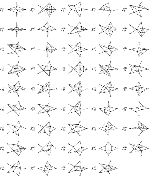
Figure 7: Four loop five-point parity even amplitude graphs.

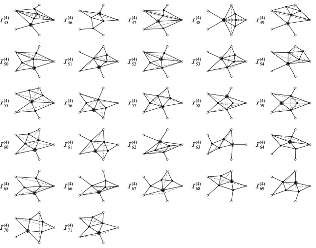
Figure 8: Four loop five-point parity odd amplitude graphs. A starred vertex $v$ indicates a factor $i\epsilon_{12345v}$.

7 Relation to other ways of writing 5-point integrands

7.1 Momentum space integrands

Forms for 1- and 2-loop 5-point amplitudes are available in momentum space in the literature both in the planar [56, 20] and more recently the full non-planar theory [21]. Whilst it is straightforward to write our dual momentum space integrands in terms of momentum space (simply using the replacement $p_{i}=x_{i\,i+1}$) a direct comparison requires some manipulation. In particular the preferred bases have integration variables appearing only as scalar products, rather than in parity odd epsilon tensors as we have here. The parity odd epsilon tensors then only depend on external momenta.

We can easily rewrite our integrands in such a form using a single formula for rewriting $\epsilon_{123456}$ in terms of $x_{i6}^{2}$ derived in appendix B.1 namely

$$\epsilon_{123456} =\frac{s_{2}s_{3}}{8\,\epsilon(p_{1},p_{2},p_{3},p_{4})}Tr(\not{p}_{4}\not{p}_{5}\not{p}_{1}\not{p}_{2})\,x_{16}^{2}\quad+\ \text{cyclic 1,2,3,4,5}$$

$$\qquad+\frac{s_{1}s_{2}s_{3}s_{4}s_{5}}{16\,\epsilon(p_{1},p_{2},p_{3},p_{4})}\ ,$$ (57)

where $p_{i}=x_{i\,i+1}$ are the amplitude momenta and $s_{i}=x_{i\,i+2}^{2}=(p_{i}+p_{i+1})^{2}$ the usual two-particle invariants. Note that this form breaks manifest dual conformal symmetry, and the coefficients of the integrands are more ugly, but it enables fairly direct comparison with results in the literature.

The canonical example is one loop. From (39) the 1 loop parity odd term is

$$\frac{i\epsilon_{123456}}{x_{16}^{2}x_{26}^{2}x_{36}^{2}x_{46}^{2}x_{56}^{2}}$$

which, using (57) becomes

$$\frac{i\,s_{2}s_{3}}{8\,\epsilon(p_{1},p_{2},p_{3},p_{4})}Tr(\not{p}_{4}\not{p}_{5}\not{p}_{1}\not{p}_{2})\,\times\,\text{Box}(p_{2},p_{3},p_{4},p_{5}+p_{1})\quad+\ \text{cyclic 1,2,3,4,5}$$

$$\qquad+\frac{i\,s_{1}s_{2}s_{3}s_{4}s_{5}}{16\,\epsilon(p_{1},p_{2},p_{3},p_{4})}\,\times\,\text{Pent}(p_{1},p_{2},p_{3},p_{4},p_{5})$$ (58)

where we see the (one mass) scalar box integrands and a scalar pentagon integrand

$$\text{Box}(p_{2},p_{3},p_{4},p_{5}+p_{1})=\int d^{4}x_{6}\frac{1}{x_{26}^{2}x_{36}^{2}x_{46}^{2}x_{56}^{2}}\,,$$ (59)

$$\text{Pent}(p_{1},p_{2},p_{3},p_{4},p_{5})=\int d^{4}x_{6}\frac{1}{x_{16}^{2}x_{26}^{2}x_{36}^{2}x_{46}^{2}x_{56}^{2}}$$ (60)

with non-trivial coefficients. These can then be compared directly with for example with the form for non-planar amplitudes (in the planar limit) found in [21] where the same basis of scalar integrals is used and we find perfect matching.

At two loops, using the same formula we reproduce the form of the amplitude given in [20].

7.2 Twistor space integrands

General expressions for MHV amplitude integrands up to three loops (parity even and odd) have also been given in momentum twistor space [28]. We will not review momentum twistors here. The only information we will need is the relation to the six-dimensional formalism reviewed in appendix B. When the $X_{i}$ are consecutively lightlike separated (i.e. $X_{i}\cdot X_{i+1}=0$) then we let ${X}_{i}^{AB}=Z_{i-1}^{\left[A\right.}Z_{i}^{\left.B\right]}$. Now let’s consider various integrands as they are expressed in [28]. All one-loop integrands are written in terms of a dual-conformal pentagon integral:

$$I_{i,j}=\frac{\langle AB(i-1,i,i+1)\cap(j-1,j,j+1)\rangle\langle X,i,j\rangle}{\langle AB,i-1,i\rangle\langle AB,i,i+1\rangle\langle AB,j-1,j\rangle\langle AB,j,j+1\rangle\langle ABX\rangle}$$ (61)

This can be rewritten in terms of a trace over $X$ variables

$$I_{i,j}=\frac{\mathrm{Tr}(X\tilde{X}_{i+1}X_{i}\tilde{X}_{0}X_{j}\tilde{X}_{j+1})}{(X_{0}\cdot X_{i})(X_{0}\cdot X_{i+1})(X_{0}\cdot X_{j})(X_{0}\cdot X_{j+1})(X_{0}\cdot X)}\ .$$ (62)

Here the integration over twistors $A$, $B$ has become integration over the $X$-space variable $X_{0}$. The variable $X$ is a reference twistor meaning it should drop out of the sum which gives the one-loop amplitude. Indeed the simplest way to deal with it is to set it to be one of the external points, e.g. $X=X_{5}$. So the one loop amplitude can be written entirely in terms of a six-trace. Just as for the more familiar four-traces in QFT, the six-trace splits as a parity odd term $\epsilon$ and a parity even term (multiple scalar products)

$$\text{Tr}(X\tilde{X}_{i+1}X_{i}\tilde{X}_{0}X_{j}\tilde{X}_{j+1}))=4\,i\,\epsilon_{X(i+1)i0j(j+1)}+4\,(X_{0}.X)(X_{i+1}.X_{j+1})(X_{i}.X_{j})+\dots$$ (63)

where the dots indicate similar terms which can be obtained by taking all possible combinations of scalar products between the six entries of the trace with minus signs where appropriate. We see immediately that the parity odd part of this twistor integrand will yield exactly the same pentagon ${\cal I}_{2}^{(5)}$ derived from the correlator. After summing all diagrams, the parity even terms will also give the same sum over one-mass boxes we expect.

Similarly at two loops, the $n$-point momentum twistor integrand in [28] is

$$M_{5}\,=\, {{\frac{1}{2}\sum_{i<j<k<l<i}\frac{\langle AB(i-1,i,i+1)\cap(j-1,j,j+1)\rangle\langle i,j,k,l\rangle}{\langle AB,i-1,i\rangle\langle ABi,i+1\rangle\langle AB,j-1,j\rangle\langle AB,j,j+1\rangle\langle ABCD\rangle}}}$$

$$\qquad\qquad\qquad\qquad\qquad\times\frac{\langle CD(k-1,k,k+1)\cap(l-1,l,l+1)\rangle}{\langle CD,k-1,k\rangle\langle CD,k,k+1\rangle\langle CD,l-1,l\rangle\langle CD,l,l+1\rangle}$$ (64)

which we can re-write in $X$-coordinates (the integration variables are $AB=X_{0}$, $CD=X_{\bar{0}}$) in the form:

$$\frac{1}{2}\sum_{ijkl}\frac{\left[X_{i+1}\tilde{X}_{i}X_{0}\tilde{X}_{j+1}X_{j}\right]^{AB}\left[X_{k+1}\tilde{X}_{k}X_{\bar{0}}\tilde{X}_{l+1}X_{l}\right]^{CD}\epsilon_{ABCD}}{(X_{0}\cdot X_{i})(X_{0}\cdot X_{i+1})(X_{0}\cdot X_{j})(X_{0}\cdot X_{j+1})(X_{0}\cdot X_{\bar{0}})(X_{\bar{0}}\cdot X_{k})(X_{\bar{0}}\cdot X_{k+1})(X_{\bar{0}}\cdot X_{l})(X_{\bar{0}}\cdot X_{l+1})}$$ (65)

To rewrite further we take advantage of ’boundary cases’, i.e. at 5-points either $j=i+1$ or $j=i+2$ and $l=k+1$. For example when $j=i+1$ we get:

$$\frac{X_{i}.X_{i+2}\,\mathrm{Tr}(X_{\bar{0}}\tilde{X}_{k}X_{k+1}\tilde{X}_{i+1}X_{l+1}\tilde{X}_{l})}{(X_{0}\cdot X_{i})(X_{0}\cdot X_{i+1})(X_{0}\cdot X_{i+2})(X_{0}\cdot X_{\bar{0}})(X_{\bar{0}}\cdot X_{k})(X_{\bar{0}}\cdot X_{k+1})(X_{\bar{0}}\cdot X_{l})(X_{\bar{0}}\cdot X_{l+1})}$$ (66)

In this way and using (63) we indeed recover the two loop 5-point amplitude in the form (46).

At three loops, starting from the equations given in [28] we are able to reproduce the same set of graphs which we have produced here. The mapping for parity odd terms is very simple and can be seen directly from drawing graphs dual to those given in [28], however the parity even terms are significantly more complicated.

8 Conclusions

The supersymmetric correlator/amplitude duality in ${\cal N}=4$ gives a way of relating objects with different numbers of outer points, or in- or outgoing particles, respectively. In the present article we have exploited this feature of the construction to derive the integrand of the colour ordered five-point amplitude up to five (and in the parity even sector six) loops from that of the four-point function of energy-momentum multiplets, which was so far chiefly associated with the MHV four-point amplitude [47, 48].

In order to take the step from four to five points, one of the integration vertices of the four-point integrand has to be regarded as an outer point. Necessarily we lose one loop order in this way. It turns out that the five-point integrand can only be uniquely fixed by taking into account topological information: amplitude graphs are planar on the disc, while the correlator integrands also contain products of two such graphs. We have used the one-loop $\times$ higher-loop terms to gain more equations on the loop corrections to the five-point amplitude. Stripping off a one-loop amplitude implies losing another loop order, though.

A beautiful picture then emerges where the parity even five-point $\ell$-loop amplitudes correspond to the outsides of those five-cycles in the planar correlator $f^{(\ell+1)}$-graphs which have no vertices on their insides, whereas the parity odd amplitude graphs correspond to the outsides of those five-cycles in the planar correlator $f^{(\ell+2)}$-graphs which have a single vertex on their inside.

Our main new results are the four- and five-loop integrands for the five-point MHV (or in this case equivalently the NMHV) amplitude. To this end, the analysis of [48] was extended to the seven-loop integrand of the four-point correlation function of energy-momentum multiplets based on the result [29] for the four-point MHV amplitude up to seven loops. We have thus made a four-point into a five-point amplitude.

Indeed, that this picture works out to be consistent is rather remarkable and non-trivial. The duality with four-point amplitudes can be shown to be consistent as long as the corresponding amplitude graphs obey the rung rule [12] which in the correlator picture simply corresponds to gluing pyramids onto the $f$-graphs [48]. Indeed the mere existence of the four-point duality then predicts many of the coefficients of loop level amplitudes (all up to three loops, the first two out of the three four-loop $f$-graphs, and the first six out of seven five-loop $f$-graphs (see (LABEL:eq:6) etc.) What is the topological reason stopping certain four-point $f$-graphs being determined from lower loops? Recall the refined four-point duality (see footnote 4) $2F_{4;m}^{(\ell)}=M_{4}^{(m)}M_{4}^{(\ell-m)}$. Thus $f$-graphs with four-cycles with a non-trivial “inside” and “outside” (i.e. which contribute to $m>0$) are determined entirely in terms of lower loop amplitudes. Conversely $f$-graphs which give no contribution to $F_{m}^{(\ell)}$ for $m>0$, i.e. which have no such four-cycle, cannot be determined from lower loop four-point amplitudes (see the final two graphs in $f^{(4)}$ and $f^{(5)}$ in (LABEL:eq:6)).

For the five-point duality on the other hand the consistency is much more subtle and we have no clear understanding (i.e. a generalisation of the pyramid gluing rung rule) for why this works. The confusion comes from the many terms which appear when gluing two $\epsilon_{123456}$ together, many of which have to cancel. However we have noticed that the structure does indeed determine many of the non-rung-rule-determined coefficients. Indeed merely the structure and consistency of the picture determines all coefficients up to $f^{(5)}$, i.e. the mere existence of the amplitude/correlator duality at 4- and 5-points determines the four-point correlator and amplitude to five loops and the five-point amplitude to four loops (parity even) and three loops (parity odd). The first coefficient which is not determined by these purely structural arguments is that of the 10-point (6 loop) $f$-graph:

Clearly any $f$-graph giving no contribution to $F_{5;m}^{(\ell)}$ for $m>0$ (i.e. whose 5-cycles have either no vertices inside or none outside) will not be determined by lower loops and it seems likely that the converse is true also: any $f$-graph contributing to $F_{5;m}^{(5)}$ for $m>0$ will be determined from lower loops via the refined duality (26) $F_{5;m}^{(\ell)}=M_{5}^{(m)}\bar{M}_{5}^{(\ell-m)}+M_{5}^{(\ell-m)}\bar{M}_{5}^{(m)}$. Indeed we see that all the 5-cycles of the graph above have either nothing inside or nothing outside them and this is the first such $f$-graph, confirming this idea. Interestingly this graph is also the first $f$-graph with a coefficient different from $\pm 1$ it having the coefficient 2.

The integrands we find are given in a local form in configuration space, which is very closely related to the twistor integrands of [25, 28] as we demonstrated in Section 7 in the text: the twistor numerators involving parity odd parts can be rather painlessly rewritten in terms of simple squares of distances and the structure $\epsilon_{12345v}=\epsilon(X_{1}X_{2}X_{3}X_{4}X_{5}X_{v})$ where the X are coordinates on the projective light-cone in 6d related to those of Minkowski space, see appendix B. This object is conformally invariant and can be broken down to a sum of 4d terms of the type $x_{1v}^{2}\epsilon(x_{2v}x_{3v}x_{4v}x_{5v})$. In the 6d epsilon, 1,2,3,4,5 denote the outer points, and only the sixth variable is an integration point. All parity odd terms in our results are of this type; epsilon terms with more than one integration vertex do not occur. By the use of Schouten identities etc. one can remove any given point from an epsilon contraction, but at the expense of introducing further denominator factors. Hence there is freedom as to the writing of the end result, although the form we found is perhaps the most natural one since it is manifestly free of higher poles like $1/x_{ij}^{4}$.

Interestingly, it is possible to generate the parity even part of the five-point amplitude from the parity odd bit up to four-loops using a few universal rules for how to replace an epsilon term. These rules depend on the other numerator terms multiplying the $\epsilon_{12345v}$. For example clearly the one-loop result can be rewritten as a single pentagon upon replacing

$$i\epsilon_{123456}\ \rightarrow\ \Big{(}x^{2}_{16}x^{2}_{24}x^{2}_{35}+x^{2}_{26}x^{2}_{14}x^{2}_{35}+x^{2}_{36}x^{2}_{14}x^{2}_{25}+x^{2}_{46}x^{2}_{13}x^{2}_{25}+x^{2}_{56}x^{2}_{13}x^{2}_{24}+i\epsilon_{123456}\Big{)}\ .$$ (67)

This is the only parity odd graph with a numerator involving an $\epsilon$ and nothing else. Other numerators have various $x^{2}$ products multiplying. If we make the following replacements for $a,b,c>0$:

$$ix_{13}^{2a}\epsilon_{123456}\ \rightarrow\ x_{13}^{2a}\Big{(}x^{2}_{56}x^{2}_{13}x^{2}_{24}+x^{2}_{46}x^{2}_{13}x^{2}_{25}+x^{2}_{26}x^{2}_{14}x^{2}_{35}+i\epsilon_{123456}\Big{)}$$

$$ix_{13}^{2a}x_{14}^{2b}\epsilon_{123456}\ \rightarrow\ x_{13}^{2a}x_{14}^{2b}\Big{(}x^{2}_{56}x^{2}_{13}x^{2}_{24}+x^{2}_{26}x^{2}_{14}x^{2}_{35}-x^{2}_{16}x^{2}_{23}x^{2}_{45}+i\epsilon_{123456}\Big{)}$$

$$ix_{13}^{2a}x_{24}^{2b}\epsilon_{123456}\ \rightarrow\ x_{13}^{2a}x_{24}^{2b}\Big{(}x^{2}_{56}x^{2}_{13}x^{2}_{24}+x^{2}_{26}x^{2}_{14}x^{2}_{35}+x^{2}_{36}x^{2}_{14}x^{2}_{25}+i\epsilon_{123456}\Big{)}$$

$$ix_{13}^{2a}x_{14}^{2b}x_{24}^{2c}\epsilon_{123456}\ \rightarrow\ x_{13}^{2a}x_{14}^{2b}x_{24}^{2c}\Big{(}x^{2}_{56}x^{2}_{13}x^{2}_{24}+x^{2}_{26}x^{2}_{14}x^{2}_{35}+x^{2}_{36}x^{2}_{14}x^{2}_{25}$$

$$\qquad\qquad\qquad\qquad\qquad-x^{2}_{16}x^{2}_{23}x^{2}_{45}-x^{2}_{46}x^{2}_{13}x^{2}_{25}+i\epsilon_{123456}\Big{)}$$ (68)

and all forms related by cyclicty related in a similar way, then the parity odd graphs will give the parity even graphs for free up to four loops. Beyond one loop, the easiest case to check is obviously the two loop case (46) where we use the first replacement. This procedure fails for the first time at 5 loops where we are left with a single parity even graph which is not determined by the parity odd sector in this manner:

This happens to be the single five-point amplitude graph generated by the ten-point $f$-graph above whose coefficient is undetermined by consistency with the duality. So we see that these rules for obtaining parity even graphs from parity odd are intimatey related to the consistency of the whole system but we have not yet fully probed this.

Note that the twistor numerators of [25, 28] (c.f. Section 7.2) also combine even and odd graphs and so the above rewriting may give expressions closer to those. One direction for future work might indeed be to look for a universal numerator describing higher-loop $n$-point amplitudes.

Another direction for future work would be to consider the six-point light-like limit. Defining

$$F_{6}^{(\ell)}:=\text{external factor}\times\lim_{\begin{subarray}{c}x^{2}_{i\,i+1}\rightarrow 0\\ (\text{mod }6)\end{subarray}}\int d^{4}x_{7}\dots d^{4}x_{6+\ell}{f^{(\ell+2)}\over\ell!}$$ (69)

where here the external factor is ${x^{2}_{12}x^{2}_{23}x^{2}_{34}x^{2}_{45}x^{2}_{56}x^{2}_{61}x^{2}_{13}x^{2}_{24}x^{2}_{35}x^{2}_{46}x^{2}_{51}x^{2}_{62}}$ then we will find the formula

$$\sum_{\ell\geq 0}{a^{\ell}}{F_{6}^{(\ell)}}\ =\ M_{6}\overline{M}_{6}+\text{NMHV contribution}\ .$$ (70)

There are various complications arising here. Firstly the NMHV contribution needs to be separated out (although this may be possible due to singularities in $x_{14}^{2},x_{25}^{2}$ and $x_{36}^{2}$ which can only appear here and not in the MHV sector). Another complication arises since there is no longer a distinction between product graphs and disc planar graphs. The graph (one loop box)$\times$ (one loop box) can appear in a disc planar fashion and indeed does appear in the two-loop six point result. Nevertheless we have seen that one can obtain more information than appears at first sight from these considerations and this certainly deserves further investigation.

We note that there are not believed to be any $\mu$ terms at five-points and thus the results here should be valid to all orders in dimensional regularisation parameter $\epsilon$ by writing the integrals in momentum space and allowing the integration momenta to live in $4-2\,\epsilon$ dimensions.

Finally, our results at five loops and beyond are contained in various attachments to the electronic version of this article, as detailed at the end of Section 6.

Appendices

Appendix A The operation “cyc[]”

It is defined to be the weighted sum over cyclically ordered (including parity flip) external points. Explicitly, for a function depending on only four out of the five external points this is defined as

$$\text{cyc}\left[f(x_{1},x_{2},x_{3},x_{4})\right]:=\sum_{1\leq i<j<k<l<i+5\leq 10}{f(x_{i},x_{j},x_{k},x_{l})+f(x_{l},x_{k},x_{j},x_{i})\over\text{symmetry factor}[f]}$$ (71)

whereas for a 5-point function it is defined as

$$\begin{split}\text{cyc}\left[f(x_{1},x_{2},x_{3},x_{4},x_{5})\right]&:=\sum_{1\leq i<j<k<l<m<i+5\leq 10}{f(x_{i},x_{j},x_{k},x_{l},x_{m})+f(x_{m},x_{l},x_{k},x_{j},x_{i})\over\text{symmetry factor}[f]}\\ &=\sum_{i=1}^{5}{f(x_{i},x_{i+1},x_{i+2},x_{i+3},x_{i+4})+f(x_{i+4},x_{i+3},x_{i+2},x_{i+1},x_{i})\over\text{symmetry factor}[f]}\ .\end{split}$$ (72)

Here all points are external and are mod 5. The symmetry factor is defined as the number of terms left invariant under such permutations. So for example, for a four-point function

$$\text{symmetry factor}\left[f(x_{1},x_{2},x_{3},x_{4})\right]= \Big{|}\big{\{}f(x_{i},x_{j},x_{k},x_{l})=f(x_{1},x_{2},x_{3},x_{4}):{\scriptstyle 1\leq i<j<k<l<i+5\leq 10}\big{\}}\Big{|}$$

$$+\Big{|}\big{\{}f(x_{l},x_{k},x_{j},x_{i})=f(x_{1},x_{2},x_{3},x_{4}):{\scriptstyle 1\leq i<j<k<l<i+5\leq 10}\big{\}}\Big{|}$$ (73)

and similarly for a five-point function. Note that this insures that the argument of the operation cyc$[]$ always appears with weight 1 when expanding the result into inequivalent terms, i.e.

$$\text{cyc}[f(x_{1},x_{2},x_{3},x_{4})]=f(x_{1},x_{2},x_{3},x_{4})+\dots$$ (74)

Finally we note that we will be dealing with integrands in general. We define integrands to be equal if they are equal up to a permutation of internal points, i.e. our functions have hidden dependence on internal variables $f(x_{1},x_{2},x_{3},x_{4},x_{5})=f(x_{1},x_{2},x_{3},x_{4},x_{5};x_{6},\dots x_{5+\ell})$ and we say

$$f(x_{1},x_{2},x_{3},x_{4},x_{5}) =f(x_{i},x_{j},x_{k},x_{l},x_{m})$$

$$\Updownarrow$$ (75)

$$f(x_{1},x_{2},x_{3},x_{4},x_{5};x_{6},x_{7},\dots x_{5+\ell}) =f(x_{i},x_{j},x_{k},x_{l},x_{m};x_{\sigma_{6}},x_{\sigma_{7}},\dots x_{\sigma_{5+\ell}})$$

for some permutation $\sigma$ of the internal variables $x_{6},\dots x_{5+\ell}$.

Appendix B 4d Minkowski coordinates in 6d $X$-variables

In order to relate our five-point integrands to similar twistor integrands found in the literature and also to explain the origin of $\epsilon_{12345v}$ used for our parity odd integrands, it is extremely useful to view 4-dimensional Minkowski space as the (Klein) quadric inside $\mathbb{RP}^{5}$. This, and its relation to momentum twistors in the context of dual conformal symmetry for amplitudes was introduced in [55].

Specifically we can describe Minkowski space in terms of six projective coordinates $X_{I}$ living in 2+4 dimensions and satisfying the null condition

$$X_{-1}^{2}+X_{0}^{2}-X_{1}^{2}-X_{2}^{2}-X_{3}^{2}-X_{4}^{2}=0$$ (76)

As such the conformal group SO(2,4) then acts linearly on these coordinates. The four-dimensional Minkowski space coordinates $x^{\mu}$, $\mu=0,1,2,3$ can be obtained easily from these by choosing a suitable representation for the homogeneous coordinate $X^{I}$.

$$X^{I}\sim\left(\frac{1-x^{2}}{2},x^{\mu},\frac{1+x^{2}}{2}\right)\hskip 56.9055ptI=-1,0,1,2,3,4$$ (77)

It is also useful — especially in relation to twistor integrands — to consider the spinorial representation of the $X^{I}$. Using that $SO(2,4)\sim SU(2,2)$ it is this representation which we employ later to consider the integrands. There are two versions:

$$X^{I}\rightarrow X=(\Sigma_{I})X^{I}$$

$$X^{I}\rightarrow\tilde{X}=(\tilde{\Sigma}_{I})X^{I}$$ (78)

where the $\Sigma$’s are are $4\times 4$ sigma matrices in 6 dimensions. We can choose them to satisfy

$$(\tilde{\Sigma}_{I})_{AB}=\frac{1}{2}\epsilon_{ABCD}(\Sigma_{I})^{CD}$$ (79)

giving the relation

$$\tilde{X}_{AB}=\frac{1}{2}\epsilon_{ABCD}X^{CD}.$$ (80)

The Clifford algebra relations,

$$\Sigma_{I}\tilde{\Sigma}_{J}+\Sigma_{J}\tilde{\Sigma}_{I}=\tilde{\Sigma}_{I}\Sigma_{J}+\Sigma_{I}\tilde{\Sigma}_{J}=2\,\eta_{IJ}$$ (81)

where $\eta_{IJ}$ is the flat metric in 2+4 dimensions, imply the following for any 6-vectors X, Y

$$X\tilde{Y}+Y\tilde{X}=2\,X\cdot Y \hskip 56.9055ptX\tilde{X}=X\cdot X\ .$$ (82)

We also have that

$$\epsilon_{IJKLMN}\Sigma_{I}\tilde{\Sigma}_{J}\Sigma_{K}\tilde{\Sigma}_{L}\Sigma_{M}\tilde{\Sigma}_{N}=i1_{4}\ .$$ (83)

B.1 Different forms for $\epsilon_{123456}$

We now consider how we are to go about writing down conformal covariants. This can be done either using vector $X$’s or spinorial $X$’s, in both cases we simply need to soak up all indices. In the vectorial notation we can essentially use $\eta_{IJ}$ or $\epsilon_{IJKLMN}$ to form invariants, those obtained using a single $\epsilon_{IJKLMN}$ will be parity-odd. The covariants for 5-points and below must necessarily be composed of only $(X_{I}\cdot X_{J})$ whereas at six-points and above we may also have the parity-odd object

$$\epsilon_{123456}:=\epsilon_{IJKLMN}X^{I}_{1}X^{J}_{2}X^{K}_{3}X^{L}_{4}X^{M}_{5}X^{N}_{6}=\det\Big{(}X_{i}{}^{I}\Big{)}$$ (84)

Indeed one can see that at six points this is the unique parity odd covariant piece. One can convert these invariants to four-dimensional notation straightforwardly by using (77)

$$X_{I}\cdot X_{J}\sim-\frac{1}{2}(x_{i}-x_{j})^{2}$$ (85)

$$\epsilon_{123456}\sim\frac{1}{2}\frac{1}{4!}\sum_{\sigma\epsilon S_{6}}(-1)^{\sigma}x_{\sigma_{1}}^{2}\epsilon(x_{\sigma_{2}},x_{\sigma_{3}},x_{\sigma_{4}},x_{\sigma_{5}})$$ (86)

Note that the latter expression for $\epsilon_{123456}$ does not look translation invariant in terms of Minkowski space variables. But of course it must be, and indeed an infinitesimal translation $x_{i}\rightarrow x_{i}+a$ gives

$$\delta\epsilon_{123456}=\sum_{\sigma\epsilon S_{6}}(-1)^{\sigma}\Big{(}a\cdot x_{\sigma_{1}}\epsilon(x_{\sigma_{2}},x_{\sigma_{3}},x_{\sigma_{4}},x_{\sigma_{5}})+2x_{\sigma_{1}}^{2}\epsilon(a,x_{\sigma_{3}},x_{\sigma_{4}},x_{\sigma_{5}})\Big{)}=0\$$ (87)

The first term vanishes due to a five term identity (expressing the fact that five points in $M^{4}$ are linearly dependent) and the second term vanishes since it is independent of $x_{\sigma_{2}}$ and $x_{\sigma_{6}}$ which appear antisymmetrically.

We can therefore rewrite the expression to make the translation invariance manifest, eg by translating by $x_{6}$ giving

$$\epsilon_{123456} \sim\frac{1}{2}\frac{1}{4!}\sum_{\sigma\epsilon S_{5}}(-1)^{\sigma}x_{\sigma_{1}\,6}^{2}\epsilon(x_{\sigma_{2}\,6},x_{\sigma_{3}\,6},x_{\sigma_{4}\,6},x_{\sigma_{5}\,6})\ .$$ (88)

It is also useful however (to compare with results in the literature which are often written in terms of scalar integrals) to give another writing of the object $\epsilon_{123456}$.

For this we first define the 6-vector $Y$ as

$$Y_{I}=\epsilon_{IJKLMN}X_{1}^{J}X_{2}^{K}X_{3}^{L}X_{4}^{M}X_{5}^{N}$$ (89)

so that $\epsilon_{123456}=-Y.X_{6}$ and then we decompose $Y$ in terms of the five vectors $X_{i}$ and the vector $I=(1,0,0,0,0,-1)$ which represents infinity in Minkowski space. Including infinity breaks conformal invariance but allows us to write all integrands in terms of purely scalar integrands which is common in the literature.

So we write

$$Y=\sum_{i=1}^{5}\alpha_{i}X_{i}+\beta I$$ (90)

and if we can solve for the coefficients $\alpha_{i},\beta$ we thus have an expression for $\epsilon_{123456}$ as

$$\epsilon_{123456}=-\sum_{i=1}^{5}\alpha_{i}X_{i}.X_{6}-\beta=1/2\sum_{i=1}^{5}\alpha_{i}x_{i6}^{2}-\beta\ .$$ (91)

To solve for by the $\alpha_{i},\beta$ simply dot (90) with $X_{j},Y$, to obtain the matrix equation

$$\left(\left(\begin{array}[]{c}X_{i}\\ I\end{array}\right).(X_{j},I)\right)\left(\begin{array}[]{c}\alpha_{i}\\ \beta\end{array}\right)=\left(\begin{array}[]{c}0\\ Y.I\end{array}\right)$$ (98)

where we use that $X_{j}.I=1$. Noting further that

$$Y.I=-\det\left(\begin{array}[]{c}X_{i}{}^{I}\\ I^{I}\end{array}\right)=\frac{1}{4!}\sum_{i\in S_{5}}(-1)^{\sigma}\epsilon(x_{\sigma_{1}},x_{\sigma_{2}},x_{\sigma_{3}},x_{\sigma_{4}})=\epsilon(x_{12},x_{23},x_{34},x_{45})\ ,$$ (101)

where the last equation can be obtained by simply expanding out the right-hand side which will be recognised as $\epsilon(p_{1},p_{2},p_{3},p_{4})$ in momentum space. Further useful equations straightforward to derive are

$$\det(X_{i}.X_{j}) =-\frac{1}{16}x_{13}^{2}x_{24}^{2}x_{35}^{2}x_{41}^{2}x_{52}^{2}$$ (102)

$$\det\left(\left(\begin{array}[]{c}X_{i}\\ I\end{array}\right).(X_{j},I)\right) =\det\left(\begin{array}[]{c}X_{i}{}^{I}\\ I^{I}\end{array}\right)^{2}=\epsilon(x_{12},x_{23},x_{34},x_{45})^{2}\ .$$ (107)

(Note that the first equation above is the only one which is not valid for arbitrary values of space-time points $X_{i}$, but only in the five-point light-like limit where $X_{i}.X_{i+1}=0$.): Thus inverting (98) and using these formulae we obtain

$$\alpha_{1} =\frac{-x^{2}_{24}x^{2}_{35}\left(x_{13}^{2}x_{52}^{2}-x^{2}_{24}x^{2}_{13}+x^{2}_{35}x^{2}_{24}-x^{2}_{41}x^{2}_{35}+x^{2}_{52}x^{2}_{41}\right)}{16\,\epsilon(x_{12},x_{23},x_{34},x_{45})}\qquad\text{and cyclic for }\alpha_{2},\dots\alpha_{5}$$

$$\beta =\frac{-x^{2}_{13}x^{2}_{24}x^{2}_{35}x^{2}_{41}x^{2}_{52}}{16\,\epsilon(x_{12},x_{23},x_{34},x_{45})}\ .$$ (108)

The $\alpha_{i}$ can be further rewritten in the simpler form in momentum space via

$$\alpha_{1}=\frac{s_{2}s_{3}}{4\,\epsilon(p_{1},p_{2},p_{3},p_{4})}Tr(\not{p}_{4}\not{p}_{5}\not{p}_{1}\not{p}_{2})\quad\text{and cyclic for }\alpha_{2},\dots\alpha_{5}$$ (109)

where $p_{i}=x_{i\,i+1},\ s_{i}=x_{i\,i+2}^{2}=(p_{i}+p_{i+1})^{2}$.

References

- [1] Z. Bern, L. J. Dixon, D. C. Dunbar and D. A. Kosower, Nucl. Phys. B 425 (1994) 217 [hep-ph/9403226].
- [2] Z. Bern, L. J. Dixon, D. C. Dunbar and D. A. Kosower, Nucl. Phys. B 435 (1995) 59 [hep-ph/9409265].
- [3] R. Britto, F. Cachazo and B. Feng, Nucl. Phys. B 725 (2005) 275 [hep-th/0412103].
- [4] E. I. Buchbinder and F. Cachazo, JHEP 0511 (2005) 036 [hep-th/0506126].
- [5] J. M. Drummond, J. Henn, G. P. Korchemsky and E. Sokatchev, Nucl. Phys. B 795 (2008) 52 [arXiv:0709.2368 [hep-th]].
- [6] J. M. Drummond, J. Henn, G. P. Korchemsky and E. Sokatchev, Nucl. Phys. B 826 (2010) 337 [arXiv:0712.1223 [hep-th]].
- [7] J. M. Drummond, J. Henn, G. P. Korchemsky and E. Sokatchev, Nucl. Phys. B 828 (2010) 317 [arXiv:0807.1095 [hep-th]].
- [8] A. Brandhuber, P. Heslop and G. Travaglini, Phys. Rev. D 78 (2008) 125005 [arXiv:0807.4097 [hep-th]].
- [9] A. Brandhuber, P. Heslop and G. Travaglini, JHEP 0910 (2009) 063 [arXiv:0906.3552 [hep-th]].
- [10] Z. Bern, J. J. M. Carrasco and H. Johansson, Phys. Rev. D 78 (2008) 085011 [arXiv:0805.3993 [hep-ph]].
- [11] Z. Bern, J. J. M. Carrasco and H. Johansson, Phys. Rev. Lett. 105 (2010) 061602 [arXiv:1004.0476 [hep-th]].
- [12] Z. Bern, J. S. Rozowsky and B. Yan, Phys. Lett. B 401 (1997) 273 [hep-ph/9702424].
- [13] Z. Bern, L. J. Dixon and V. A. Smirnov, Phys. Rev. D 72 (2005) 085001 [hep-th/0505205].
- [14] Z. Bern, M. Czakon, L. J. Dixon, D. A. Kosower and V. A. Smirnov, Phys. Rev. D 75 (2007) 085010 [hep-th/0610248].
- [15] Z. Bern, J. J. M. Carrasco, H. Johansson and D. A. Kosower, Phys. Rev. D 76 (2007) 125020 [arXiv:0705.1864 [hep-th]].
- [16] Z. Bern, L. J. Dixon, D. C. Dunbar, M. Perelstein and J. S. Rozowsky, Nucl. Phys. B 530 (1998) 401 [hep-th/9802162].
- [17] Z. Bern, J. J. M. Carrasco, L. J. Dixon, H. Johansson and R. Roiban, Phys. Rev. D 78 (2008) 105019 [arXiv:0808.4112 [hep-th]].
- [18] Z. Bern, J. J. M. Carrasco, L. J. Dixon, H. Johansson and R. Roiban, Phys. Rev. D 82 (2010) 125040 [arXiv:1008.3327 [hep-th]].
- [19] Z. Bern, J. J. M. Carrasco, H. Johansson and R. Roiban, Phys. Rev. Lett. 109 (2012) 241602 [arXiv:1207.6666 [hep-th]].
- [20] Z. Bern, M. Czakon, D. A. Kosower, R. Roiban and V. A. Smirnov, Phys. Rev. Lett. 97 (2006) 181601 [hep-th/0604074].
- [21] J. J. .Carrasco and H. Johansson, Phys. Rev. D 85 (2012) 025006 [arXiv:1106.4711 [hep-th]].
- [22] M. Spradlin, A. Volovich and C. Wen, Phys. Rev. D 78 (2008) 085025 [arXiv:0808.1054 [hep-th]].
- [23] Z. Bern, L. J. Dixon, D. A. Kosower, R. Roiban, M. Spradlin, C. Vergu and A. Volovich, Phys. Rev. D 78 (2008) 045007 [arXiv:0803.1465 [hep-th]].
- [24] F. Cachazo, M. Spradlin and A. Volovich, Phys. Rev. D 78 (2008) 105022 [arXiv:0805.4832 [hep-th]].
- [25] N. Arkani-Hamed, J. L. Bourjaily, F. Cachazo, S. Caron-Huot and J. Trnka, JHEP 1101 (2011) 041 [arXiv:1008.2958 [hep-th]].
- [26] R. Britto, F. Cachazo and B. Feng, Nucl. Phys. B 715 (2005) 499 [hep-th/0412308]; R. Britto, F. Cachazo, B. Feng and E. Witten, Phys. Rev. Lett. 94 (2005) 181602 [hep-th/0501052].
- [27] N. Arkani-Hamed, J. L. Bourjaily, F. Cachazo, A. B. Goncharov, A. Postnikov and J. Trnka, arXiv:1212.5605 [hep-th].
- [28] N. Arkani-Hamed, J. L. Bourjaily, F. Cachazo and J. Trnka, arXiv:1012.6032 [hep-th].
- [29] J. L. Bourjaily, A. DiRe, A. Shaikh, M. Spradlin and A. Volovich, JHEP 1203 (2012) 032 [arXiv:1112.6432 [hep-th]].
- [30] J. Golden and M. Spradlin, JHEP 1205 (2012) 027 [arXiv:1203.1915 [hep-th]].
- [31] L. F. Alday and J. M. Maldacena, JHEP 0706 (2007) 064 [arXiv:0705.0303 [hep-th]].
- [32] J. M. Drummond, G. P. Korchemsky and E. Sokatchev, Nucl. Phys. B 795 (2008) 385 [arXiv:0707.0243 [hep-th]].
- [33] A. Brandhuber, P. Heslop and G. Travaglini, Nucl. Phys. B 794 (2008) 231 [arXiv:0707.1153 [hep-th]].
- [34] J. M. Drummond, J. Henn, G. P. Korchemsky and E. Sokatchev, Nucl. Phys. B 815 (2009) 142 [arXiv:0803.1466 [hep-th]].
- [35] B. Eden, G. P. Korchemsky and E. Sokatchev, JHEP 1112 (2011) 002 [arXiv:1007.3246 [hep-th]].
- [36] L. F. Alday, B. Eden, G. P. Korchemsky, J. Maldacena and E. Sokatchev, JHEP 1109 (2011) 123 [arXiv:1007.3243 [hep-th]].
- [37] B. Eden, G. P. Korchemsky and E. Sokatchev, Phys. Lett. B 709 (2012) 247 [arXiv:1009.2488 [hep-th]].
- [38] B. Eden, P. Heslop, G. P. Korchemsky and E. Sokatchev, Nucl. Phys. B 869 (2013) 329 [arXiv:1103.3714 [hep-th]].
- [39] B. Eden, P. Heslop, G. P. Korchemsky and E. Sokatchev, Nucl. Phys. B 869 (2013) 378 [arXiv:1103.4353 [hep-th]].
- [40] L. J. Mason and D. Skinner, JHEP 1012 (2010) 018 [arXiv:1009.2225 [hep-th]].
- [41] S. Caron-Huot, JHEP 1107 (2011) 058 [arXiv:1010.1167 [hep-th]].
- [42] T. Adamo, M. Bullimore, L. Mason and D. Skinner, JHEP 1108 (2011) 076 [arXiv:1103.4119 [hep-th]].
- [43] J. Maldacena, Adv. Theor. Math. Phys. 2 (1998) 231 [arXiv:hep-th/9711200]; S. Gubser, I. Klebanov and A. Polyakov, Phys. Lett. B 428 (1998) 105 [arXiv:hep-th/9802109]; E. Witten, Adv. Theor. Math. Phys. 2 (1998) 253 [arXiv:hep-th/9802150].
- [44] B. Eden, A. C. Petkou, C. Schubert and E. Sokatchev, Nucl. Phys. B 607 (2001) 191 [hep-th/0009106].
- [45] F. Gonzalez-Rey, I. Y. Park and K. Schalm, Phys. Lett. B 448 (1999) 37 [hep-th/9811155]; B. Eden, P. S. Howe, C. Schubert, E. Sokatchev and P. C. West, Nucl. Phys. B 557 (1999) 355 [hep-th/9811172]; Phys. Lett. B 466 (1999) 20 [hep-th/9906051];
- [46] B. Eden, C. Schubert and E. Sokatchev, Phys. Lett. B 482 (2000) 309 [hep-th/0003096]; M. Bianchi, S. Kovacs, G. Rossi and Y. S. Stanev, Nucl. Phys. B 584 (2000) 216 [hep-th/0003203].
- [47] B. Eden, P. Heslop, G. P. Korchemsky and E. Sokatchev, Nucl. Phys. B 862 (2012) 193 [arXiv:1108.3557 [hep-th]].
- [48] B. Eden, P. Heslop, G. P. Korchemsky and E. Sokatchev, Nucl. Phys. B 862 (2012) 450 [arXiv:1201.5329 [hep-th]].
- [49] B. Eden, P. Heslop, G. P. Korchemsky, V. A. Smirnov and E. Sokatchev, Nucl. Phys. B 862 (2012) 123 [arXiv:1202.5733 [hep-th]].
- [50] C. Taylor, “Graph Theory Applied to Quantum Field Theory,” Durham University Department of Mathematical Sciences Project IV 2013; The result can be found attached to the arXiv version of this paper in the folder 7LoopResult.
- [51] P. S. Howe and G. G. Hartwell, Class. Quant. Grav. 12 (1995) 1823.
- [52] G. G. Hartwell and P. S. Howe, Int. J. Mod. Phys. A 10 (1995) 3901 [hep-th/9412147].
- [53] A. S. Galperin, E. A. Ivanov, V. I. Ogievetsky and E. S. Sokatchev, Cambridge, UK: Univ. Pr. (2001) 306 p
- [54] A. Hodges, JHEP 1305 (2013) 135 [arXiv:0905.1473 [hep-th]].
- [55] L. J. Mason and D. Skinner, JHEP 0911 (2009) 045 [arXiv:0909.0250 [hep-th]].
- [56] Z. Bern, L. J. Dixon, D. C. Dunbar and D. A. Kosower, Phys. Lett. B 394 (1997) 105 [hep-th/9611127].