Magnetic excitation in resonant inelastic x-ray scattering of Sr₂IrO₄: A localized spin picture

Abstract

We study the magnetic excitations in 5d transition-metal oxide Sr₂IrO₄ on the basis of the Heisenberg model with small anisotropic terms on a square lattice. We calculate the correlation functions by using the Green’s functions in the spin-wave approximation. The spin waves are split into two modes with slightly different energies due to the anisotropic terms. It is shown that the spin correlation functions of the $y$ and $z$ components are composed of a single peak corresponding to each mode. We analyze the process of resonant inelastic x-ray scattering (RIXS) without relying on the fast collision approximation to obtain the local scattering operator. The RIXS intensity is derived as a sum of the correlation functions of the $y$ and $z$ spin components. We demonstrate that the RIXS intensity as a function of energy shows two-peak structure brought about by the two modes, which could be observed in the RIXS experiment.

I Introduction

The $5d$ transition-metal compounds have recently drawn much attention because of the interplay between the spin-orbit interaction (SOI) and the electron correlation. Among them, Sr₂IrO₄ is one of the most fascinating systems due to the structural and electronic similarities to the La₂CuO₄, parent compound of the high-$T_{\textrm{C}}$ superconductors. This magnetic insulator, which exhibits a canted antiferromagnetic phase below $\sim$ 230 K, is proposed to be a system with an effective total angular momentum $j_{\textrm{eff}}=1/2$. Crawford et al. (1994); Cao et al. (1998); Moon et al. (2006); Clancy et al. (2012); Ye et al. (2013); Dhital et al. (2013) Many-body theoretical methods have been applied to the system to describe the electronic structure.Kim et al. (2008); Arita et al. (2012); Watanabe et al. (2010)

In the strong coupling scheme, the localized electron picture may be useful to describe the low-lying excitations in such spin-orbit induced antiferromagnetic insulator. This picture starts from the description of electronic states of each Ir atom, where five $5d$ electrons in Ir⁴⁺ ion are occupied in the $t_{2g}$ orbitals, since the energy of the $e_{g}$ orbitals is about 2 eV higher than that of the $t_{2g}$ orbitals due to the strong crystal field.Kim et al. (2008) This situation may be regarded as one hole is sitting on the t_2g orbitals. Under the strong SOI, the lowest-energy states of a hole are Kramers’ doublet with $j_{\rm eff}=1/2$.Kim et al. (2008, 2009)

The degeneracy is lifted by the inter-site interaction. Introducing the isospin operators acting on the doublet, the effective spin Hamiltonian describing the low-lying excitations is derived by the second-order perturbation with respect to the electron-transfer terms, as has usually been carried out in the superexchange theory. Anderson (1959) A Heisenberg Hamiltonian is obtained with the isotropic antiferromagnetic coupling consistent with the above findings,Jackeli and Khaliullin (2009); Jin et al. (2009); Kim et al. (2012a) as well as small anisotropic terms, which arise when Hund’s coupling is taken into account on the two-hole states in the intermediate state of the second-order perturbation.Jackeli and Khaliullin (2009); Kim et al. (2012a) Since the anisotropic terms favor the staggered moment lying in the $ab$ plane, the staggered moment is assumed to direct along the $x$ axis in the local coordinate frames. This leads to a zig-zag alignment of staggered moment along the crystal $a$ axis, because the base states are defined in the local coordinate frames rotated with respect to the $c$ axis about $\theta=\pm 11^{\circ}$ in accord with the rotation of the IrO₆ octahedra.Jackeli and Khaliullin (2009); Wang and Senthil (2011) On this situation, we have calculated the excitation spectra within the linear spin-wave approximationHolstein and Primakoff (1940) in our previous paper.Igarashi and Nagao (2013a) Having introduced the Green’s functions including the so-called anomalous type,Bulut et al. (1989) we have solved the coupled equations of motion for the Green’s functions. We have found that magnon modes in the isotropic Heisenberg model are split into two modes with slightly different energy in the entire Brillouin zone, due to the anisotropic terms. This may be considered as a hallmark of the interplay between the SOI and Hund’s coupling.

Usually, inelastic neutron scattering (INS) works effective to probe such magnetic excitations. However, it is not the case for this system, since the Ir atom is a strong absorber of neutron. On the other hand, resonant inelastic x-ray scattering (RIXS) has recently emerged as a useful probe for detecting the magnetic excitations. It has detected the single-magnon excitations as well as the two-magnon excitations in undoped cuprates, where the spectral peak behaves like the dispersion relation of spin wave in the Heisenberg model as a function of momentum transfer.Braicovich et al. (2009, 2010); Guarise et al. (2010) For Sr₂IrO₄, the RIXS experiments have also been carried out around the Ir L₃ edge.Ishii et al. (2011); Kim et al. (2012b) A low-energy peak arising from one-magnon excitations has been observed similar to undoped cuprates,Kim et al. (2012b) but no indication of the mode splitting has been seen. The theoretical analysis in the spin-wave approximation has been carried out, having described well the spectra, but without considering the anisotropic terms.Ament et al. (2011) At present, it is not clear how the split modes due to the anisotropic terms could be observed in the RIXS spectra. The purpose of this paper is to clarify the origin of two modes and how they are detected.

To this end, we introduce a pair of combination of spin operators ${\bf S}_{a}\pm{\bf S}_{b}$ where ${\bf S}_{a}$ and ${\bf S}_{b}$ are the spin operators at A and B sites, respectively. We call ${\bf S}_{a}+{\bf S}_{b}$ and ${\bf S}_{a}-{\bf S}_{b}$ as bonding and antibonding combinations, respectively. We consider the correlation functions of them, which are connected to the Green’s functions mentioned above. Since the staggered moment aligns along the $x$ axis, the correlation function of the $x$ spin component, which consists of two-magnon excitations, could be neglected as a higher order correction of $1/S$ expansion. We find that the bonding-combination functions of the $y$ and $z$ spin components consist of a single $\delta$-function peak corresponding to each mode. The modes corresponding to the $y$ and $z$ spin components are interchanged in the antibonding-combination functions.

These correlation functions are combined in evaluating the RIXS spectra. Analyzing the second-order RIXS process similar to the case for undoped cuprates,Igarashi and Nagao (2012) we obtain the expression of the local scattering operator described in terms of the spin operators at the core-hole site. The operator consists of a term consistent with the fast collision approximation (FCA)Ament et al. (2007, 2009); Haverkort (2010) and an extra term not given by FCA. However, since the lifetime broadening width is larger than the magnon energies at the Ir L edge, the latter term is considered quite small and could be neglected in the present system. Using the local scattering operator derived, we can express the RIXS spectra as a sum of the correlation functions of $y$ and $z$ spin components. Since the $\delta$-function peak energy is different between the functions with the spin components, the RIXS spectra are made up of two peaks. We also find that the correlation function of the antibonding spin combination for the momentum transfer ${\bf q}$ inside the magnetic Brillouin zone (MBZ) leads to the divergence of the intensity at ${\bf q}=(0,0)$. It attributes to the zig-zag arrangement of the staggered moment, which is a consequence of the rotation of IrO₆ octahedra. Evaluating the spectra in the model with the reasonable parameter values, we demonstrate that the mode splitting could be distinguished.

This paper is organized as follows. In Sec. II, we introduce the spin Hamiltonian with anisotropic terms in the square lattice. The excitation spectra are calculated in the spin-wave approximation with the help of the Green’s functions. The correlation functions are evaluated for the bonding and antibonding spin combinations. In Sec. III, the RIXS process is analyzed at a single site without relying on the FCA. In Sec. IV, the RIXS spectra are calculated for Sr₂IrO₄. Section V is devoted to the concluding remarks. In Appendix, the symmetry relations among the Green’s functions are summarized.

II Magnetic excitations for Sr₂IrO₄

II.1 Spin Hamiltonian

The crystal structure of Sr₂IrO₄ belongs to the K₂NiF₄ type. Crawford et al. (1994) The IrO₂-layer forms two-dimensional plane similar to the CuO₂-layer in La₂CuO₄. The crystal field energy of the $e_{g}$ orbitals is about 2 eV higher than that of the $t_{2g}$ orbitals. This yields five electrons to be occupied on $t_{2g}$ orbitals in each Ir atoms. This state could be considered as occupying one hole. The matrices of the orbital angular momentum operators with $L=2$ represented by the $t_{2g}$ states are the minus of those with $L=1$ represented by $|p_{x}\rangle$, $|p_{y}\rangle$, and $|p_{z}\rangle$, if the bases are identified by $|yz\rangle$, $|zx\rangle$, and $|xy\rangle$, respectively.Kanamori (1957) Therefore, the six-fold degenerate states are split into the states with the effective angular momentum $j_{\rm eff}=1/2$ and $3/2$ under SOI. The lowest-energy states are the doublet with $j_{\rm eff}=1/2$, given by

$$\left|\uparrow\right\rangle = \frac{1}{\sqrt{3}}\left[|yz\downarrow\rangle+i|zx\downarrow\rangle+|xy\uparrow\rangle\right],$$ (1)

$$\left|\downarrow\right\rangle = \frac{1}{\sqrt{3}}\left[|yz\uparrow\rangle-i|zx\uparrow\rangle-|xy\downarrow\rangle\right].$$ (2)

where the base states are defined in the local coordinate frames rotated in accordance with the rotation of the IrO₆ octahedra. Jackeli and Khaliullin (2009); Wang and Senthil (2011)

The exchange interaction with neighboring doublets is evaluated from the perturbation with respect to the electron transfer in the strong coupling theory.Jackeli and Khaliullin (2009); Kim et al. (2012a) By introducing the spin operators ${\bf S}$ acting on the doublet, the effective Hamiltonian may be expressed as

$$H=H^{(0)}+H^{(1)},$$ (3)

with

$$H^{(0)} = J_{\rm ex}\sum_{\langle i,j\rangle}{\bf S}_{i}\cdot{\bf S}_{j}+J^{\prime}_{\rm ex}\sum_{\langle i^{\prime},j^{\prime}\rangle}{\bf S}_{i^{\prime}}\cdot{\bf S}_{j^{\prime}}$$ (4)

$$+ J^{\prime\prime}_{\rm ex}\sum_{\langle i^{\prime\prime},j^{\prime\prime}\rangle}{\bf S}_{i^{\prime\prime}}\cdot{\bf S}_{j^{\prime\prime}}+\cdots,$$

$$H^{(1)} = J^{\prime}_{z}\sum_{\langle i,j\rangle}S_{i}^{z}S_{j}^{z}+J^{\prime}_{xy}\sum_{\langle i,j\rangle}\textrm{sgn}(i,j)\left(S_{i}^{x}S_{j}^{x}-S_{i}^{y}S_{j}^{y}\right).$$

The $H^{(0)}$ describes the isotropic exchange energy where the exchange couplings between the first, second, and third nearest-neighbors are denoted as $J_{\rm ex}$, $J^{\prime}_{\rm ex}$, and $J^{\prime\prime}_{\rm ex}$, respectively. The summations $\langle i,j\rangle$, $\langle i^{\prime},j^{\prime}\rangle$, and $\langle i^{\prime\prime},j^{\prime\prime}\rangle$ run over the first, second, and third nearest-neighbor pairs, respectively. It is known that the experimental dispersion curve can be reproduced well by setting $J_{\textrm{ex}}=60$ meV, $J_{\textrm{ex}}^{\prime}=-J_{\textbf{ex}}/3$ and $J_{\textrm{ex}}^{\prime\prime}=J_{\textbf{ex}}/4$ in the phenomenological model. Kim et al. (2012b) The $H^{(1)}$ describes the anisotropic exchange energy, which arises from the interplay between the SOI and Hund’s coupling, where $\textrm{sgn}(i,j)$ gives $+1(-1)$ when the bond between the sites $i$ and $j$ is along the $x$ ($y$) axis. It is known that $J^{\prime}_{z}$ is negative and its absolute value is nearly the same as that of $J^{\prime}_{xy}$. Jackeli and Khaliullin (2009); Kim et al. (2012a); Igarashi and Nagao (2013a) It may be sufficient to restrict the anisotropic interaction within the nearest neighbors, since it is one order of magnitude smaller than the isotropic term.

II.2 The ground state

In the absence of the anisotropic term $H^{(1)}$, the conventional antiferromagnetic spin configuration is expected, in which the direction of the staggered moment is not determined. The first term of $H^{(1)}$ makes the direction favor the $xy$ plane when $J^{\prime}_{z}<0$. This antiferromagnetic order breaks the rotational invariance of the isospin space in the $ab$ plane. We assume the staggered moment pointing to the $x$ axis.Cao et al. (1998) It should be noted here that the antiferromagnetic order in the local coordinate frames indicates a zig-zag alignment of the staggered moment, leading to the presence of the weak ferromagnetic moment in the coordinate frame fixed to the crystal axes.

II.3 Excited states

A spin-wave theory has been developed to describe excited states in Ref. Igarashi and Nagao, 2013a. Relabeling the $x$, $y$, and $z$ axes as $z^{\prime}$, $x^{\prime}$, and $y^{\prime}$ axes, respectively, we express the spin operators by boson operators within the lowest order of $1/S$-expansion:Holstein and Primakoff (1940)

$$S_{i}^{z^{\prime}} = S-a_{i}^{\dagger}a_{i},\quad S_{i}^{x^{\prime}}+iS_{i}^{y^{\prime}}=\sqrt{2S}a_{i},$$ (6)

$$S_{j}^{z^{\prime}} = -S+b_{j}^{\dagger}b_{j},\quad S_{j}^{x^{\prime}}+iS_{j}^{y^{\prime}}=\sqrt{2S}b_{j}^{\dagger},$$ (7)

where $a_{i}$ and $b_{j}$ are boson annihilation operators, and $i$ ($j$) refers to sites on the A (B) sublattice. Then, the Fourier transforms of spin operators are defined in the MBZ as

$${\bf S}_{a}({\bf k}) = \sqrt{\frac{2}{N}}\sum_{i}{\bf S}_{i}\exp(-i{\bf k}\cdot{\bf r}_{i}),$$ (8)

$${\bf S}_{b}({\bf k}) = \sqrt{\frac{2}{N}}\sum_{j}{\bf S}_{j}\exp(-i{\bf k}\cdot{\bf r}_{j}),$$ (9)

where $N$ is the number of sites, and $i$ ($j$) runs over A (B) sublattice. Defining similarly the Fourier transform of boson operators $a({\bf k})$ and $b({\bf k})$, we express the Hamiltonian as

$$H^{(0)}=J_{\rm ex}Sz\sum_{\bf k}\left\{a^{\dagger}({\bf k})a({\bf k})+b^{\dagger}({\bf k})b({\bf k})\right.$$

$$\left.+\gamma({\bf k})[a^{\dagger}({\bf k})b^{\dagger}({\bf-k})+a({\bf k})b({\bf-k})]\right\}$$

$$- J^{\prime}_{\rm ex}Sz\sum_{\bf k}[1-\gamma^{\prime}({\bf k})][a^{\dagger}({\bf k})a({\bf k})+b^{\dagger}({\bf k})b({\bf k})]$$

$$- J^{\prime\prime}_{\rm ex}Sz\sum_{\bf k}[1-\gamma^{\prime\prime}({\bf k})][a^{\dagger}({\bf k})a({\bf k})+b^{\dagger}({\bf k})b({\bf k})],$$

$$H^{(1)}=J^{\prime}_{z}(2S)\sum_{\bf k}\gamma({\bf k})[a({\bf k})-a^{\dagger}({\bf-k})][b({\bf-k})-b^{\dagger}({\bf k})]$$

$$- J^{\prime}_{xy}(2S)\sum_{\bf k}\eta({\bf k})[a({\bf k})+a^{\dagger}({\bf-k})][b({\bf-k})+b^{\dagger}({\bf k})],$$ (11)

where

$$\gamma({\bf k}) = \frac{1}{2}(\cos k_{x}+\cos k_{y}),$$ (12)

$$\gamma^{\prime}(\bf{k}) = \cos k_{x}\cos k_{y},$$ (13)

$$\gamma^{\prime\prime}(\bf{k}) = \frac{1}{2}[\cos(2k_{x})+\cos(2k_{y})],$$ (14)

$$\eta({\bf k}) = \frac{1}{2}(\cos k_{x}-\cos k_{y}).$$ (15)

Here $z$ is the number of nearest neighbors, i.e., $z=4$.

To find out the excitation modes, we introduce the Green’s functions,

$$G_{aa}({\bf k},t) = -i\langle T[a({\bf k},t)a^{\dagger}({\bf k},0)]\rangle,$$ (16)

$$F_{ba}({\bf k},t) = -i\langle T[b^{\dagger}({\bf-k},t)a^{\dagger}({\bf k},0)]\rangle,$$ (17)

$$G_{ba}({\bf k},t) = -i\langle T[b({\bf k},t)a^{\dagger}({\bf k},0)]\rangle,$$ (18)

$$F_{aa}({\bf k},t) = -i\langle T[a^{\dagger}({\bf-k},t)a^{\dagger}({\bf k},0)]\rangle,$$ (19)

where $T$ is a time-ordering operator, and $\langle X\rangle$ denotes the ground-state average of operator $X$. The $F_{ba}({\bf k},t)$ and $F_{aa}({\bf k},t)$ belong to the so called anomalous type. Their Fourier transforms are defined as $G_{aa}({\bf k},\omega)=\int G_{aa}({\bf k},t){\rm e}^{i\omega t}{\rm d}t$ and so on. Then, we get a set of equation of motion for these functions. It is given by

$$\left(\begin{array}[]{cccc}\omega-1+\xi(\textbf{k})&-A({\bf k})&B({\bf k})&0\\ -A({\bf k})&-(\omega+1-\xi(\textbf{k}))&0&B({\bf k})\\ B({\bf k})&0&\omega-1+\xi(\textbf{k})&-A({\bf k})\\ 0&B({\bf k})&-A({\bf k})&-(\omega+1-\xi(\textbf{k}))\end{array}\right)\left(\begin{array}[]{c}G_{aa}({\bf k},\omega)\\ F_{ba}({\bf k},\omega)\\ G_{ba}({\bf k},\omega)\\ F_{aa}({\bf k},\omega)\end{array}\right)=\left(\begin{array}[]{c}1\\ 0\\ 0\\ 0\end{array}\right),$$ (20)

where

$$\xi(\textbf{k}) = \frac{J_{\textrm{ex}}^{\prime}}{J_{\textrm{ex}}}(1-\gamma^{\prime}(\textbf{k}))+\frac{J_{\textrm{ex}}^{\prime\prime}}{J_{\textrm{ex}}}(1-\gamma^{\prime\prime}(\textbf{k})),$$ (21)

$$A({\bf k}) = (1+g_{z})\gamma({\bf k})-g_{xy}\eta({\bf k}),$$ (22)

$$B({\bf k}) = g_{z}\gamma({\bf k})+g_{xy}\eta({\bf k}),$$ (23)

$$g_{z} = \frac{J^{\prime}_{z}}{2J_{\rm ex}},\quad g_{xy}=\frac{J^{\prime}_{xy}}{2J_{\rm ex}}.$$ (24)

Here the energy is measured in units of $J_{\rm ex}Sz$. Hence we finally obtain,

$$\left(\begin{array}[]{c}G_{aa}({\bf k},\omega)\\ F_{ba}({\bf k},\omega)\\ G_{ba}({\bf k},\omega)\\ F_{aa}({\bf k},\omega)\\ \end{array}\right)=\frac{1}{D({\bf k},\omega)}\left(\begin{array}[]{c}g_{aa}({\bf k},\omega)\\ f_{ba}({\bf k},\omega)\\ g_{ba}({\bf k},\omega)\\ f_{aa}({\bf k},\omega)\\ \end{array}\right),$$ (25)

where

$$g_{aa}({\bf k},\omega) = [\omega-1+\xi({\bf k})][\omega+1-\xi({\bf k})]^{2}$$

$$- B({\bf k})^{2}[\omega-1+\xi({\bf k})]+A({\bf k})^{2}[\omega+1-\xi({\bf k})],$$

$$f_{ba}({\bf k},\omega) = -A({\bf k})\{\omega^{2}-[1-\xi({\bf k})]^{2}-B({\bf k})^{2}+A({\bf k})^{2}\},$$

$$g_{ba}({\bf k},\omega) = B({\bf k})\{B({\bf k})^{2}-[\omega+1-\xi({\bf k})]^{2}-A({\bf k})^{2}\},$$

$$f_{aa}({\bf k},\omega) = 2A({\bf k})B({\bf k})[1-\xi({\bf k})].$$ (29)

The denominator of Eq. (25) is given by

$$D(\textbf{k},\omega)=[\omega^{2}-E_{-}^{2}(\textbf{k})][\omega^{2}-E_{+}^{2}(\textbf{k})],$$ (30)

with

$$E_{\pm}(\textbf{k})=\sqrt{[1-\xi(\textbf{k})\pm|B(\textbf{k})|]^{2}-A^{2}(\textbf{k})}.$$ (31)

This indicates that poles exist at $\omega=E_{\pm}({\bf k})$ in the domain of $\omega>0$. When ${\bf k}\to 0$, we have $\xi({\bf k})\to 0$, $A({\bf k})\to 1+g_{z}$, and $B({\bf k})\to g_{z}$, which leads to a Goldstone mode $E_{-}(0)=0$ as well as a gap mode $E_{+}(0)=\sqrt{-2g_{z}}$. The splitting of two modes is a direct reflection of the anisotropy shown in the original Hamiltonian (LABEL:eq.H.1). Note that since $B(\textbf{k})$ is not invariant under the exchange of $k_{x}$ and $k_{y}$, the dispersion shows a slight anisotropy though the difference is negligible due to the smallness of $J_{z}^{\prime}$ and $J_{xy}^{\prime}$ in the following numerical evaluations.

Finally, evaluating the residues at the poles, we could express the Green’s function, for example, $G_{aa}({\bf k},\omega)$ as

$$G_{aa}({\bf k},\omega)=\sum_{\mu=\pm}\left\{\frac{A_{\mu}}{\omega-E_{\mu}({\bf k})+i\delta}-\frac{B_{\mu}}{\omega+E_{\mu}({\bf k})-i\delta}\right\},$$ (32)

where $\delta$ is an infinitesimal positive constant. The Green’s functions are utilized when we evaluate the spin correlation functions in the next subsection.

II.4 Spin correlation function

Since two spins exist in the unit cell, it is useful to define a pair of combination of spin operators

$${\bf Q}_{\pm}({\bf k})\equiv\frac{1}{\sqrt{2}}[{\bf S}_{a}({\bf k})\pm{\bf S}_{b}({\bf k})],$$ (33)

where $\textbf{Q}_{+}(\textbf{k})$ and $\textbf{Q}_{-}(\textbf{k})$ are called as bonding and antibonding combinations, respectively. The antibonding combination corresponds to the wave vector ${\bf k}^{\prime}={\bf k}+{\bf G}$ outside the first MBZ in the extended zone scheme, since ${\bf S}_{b}({\bf k}^{\prime})$ acquires a minus sign when it is reduced back to the first MBZ by a reciprocal lattice vector ${\bf G}$.

The INS and RIXS spectra may be connected to the correlation functions of these operators,

$$R_{\ell}^{\mu\mu}({\bf k},\omega)=\int\langle Q_{\ell}^{\mu}({\bf k},t)Q_{\ell}^{\mu}(-{\bf k},0)\rangle{\rm e}^{i\omega t}{\rm d}t,$$ (34)

with $\mu=x,y$, and $z$. Since the direction of the staggered moment is along the $x$ axis, the $R_{\ell}^{xx}({\bf k},\omega)$, composed of two-magnon excitations, is regarded as the higher order of the $1/S$ expansion, and will be neglected. The $R_{\ell}^{yy}({\bf k},\omega)$ and $R_{\ell}^{zz}({\bf k},\omega)$, composed of one-magnon excitations, are different with each other because of the anisotropic terms of $J^{\prime}_{z}$ and $J^{\prime}_{xy}$. To evaluate these functions, we decompose the right hand side of Eq. (34) into the correlation functions of Holstein-Primakoff bosons such as $\int\langle b({\bf k},t)a^{\dagger}({\bf k},0)\rangle{\rm e}^{i\omega t}{\rm d}t$, and connect them to the imaginary part of the Green’s functions such as $-2{\rm Im}\,G_{ba}({\bf k},\omega)$ for $\omega>0$. All the Green’s functions required are obtained from Eq. (25) with the help of the symmetry relations given in Appendix.

From the form of Eq. (32), we see that each correlation function has a single $\delta$-function peak structure. For instance, for k from $(0,0)$ to $(\pi,0)$, we find that $R_{+}^{zz}({\bf k},\omega)$ and $R_{-}^{zz}({\bf k},\omega)$ are composed of the $\delta$-function peaks at $E_{-}({\bf k})$ and $E_{+}({\bf k})$, respectively. On the other hand, $R_{+}^{yy}({\bf k},\omega)$ and $R_{-}^{yy}({\bf k},\omega)$ are composed of the peaks at $E_{+}({\bf k})$ and $E_{-}({\bf k})$, respectively. When we turn our attention to the diagonal direction of k, it is convenient to modify the definition of the correlation functions in the extended zone scheme. Since the antibonding combination corresponds to the wave number belonging to the outside of the first MBZ, we define the correlation functions by $R^{\mu\mu}({\bf k},\omega)\equiv R_{+}^{\mu\mu}({\bf k},\omega)$ for ${\bf k}$ inside the first MBZ, and $R^{\mu\mu}({\bf k},\omega)\equiv R_{-}^{\mu\mu}([{\bf k}],\omega)$ for ${\bf k}$ outside the 1st MBZ where $[\textbf{k}]$ is the wave vector reduced back to the first MBZ by a reciprocal lattice vector as ${\bf G}$$=\textbf{k}-[\textbf{k}]$.

In the numerical calculation, we use the parameter values, $J_{\rm ex}=60$, $J^{\prime}_{\rm ex}=-20$, $J_{\rm ex}^{\prime\prime}=15$, $J^{\prime}_{z}=-1.8$, and $J^{\prime}_{xy}=1.8$ in units of meV. The parameter set used here is the same as the one adopted in Ref. Igarashi and Nagao, 2013a, which is justified to give a better fitting of the dispersion curve of the magnetic excitation obtained by the RIXS experiment.Kim et al. (2012b) Notice that the magnitudes of the anisotropic exchange couplings $J_{z}^{\prime}$ and $J_{xy}^{\prime}$ turn out to be the same order as those evaluated by other theories.Jackeli and Khaliullin (2009); Kim et al. (2012a) Panel (a) in Fig. 1 shows the peak positions of $R^{zz}({\bf k},\omega)$ and $R^{yy}({\bf k},\omega)$ as a function of ${\bf k}$ along symmetry lines. The peak position of $R^{zz}({\bf k},\omega)$ has no gap at $(0,0)$ but has a gap at $(\pi,\pi)$, while the situation is opposite for the peak of $R^{yy}({\bf k},\omega)$. Panel (b) in Fig. 1 shows the intensities of the peaks. The intensity of $R^{zz}({\bf k},\omega)$ vanishes at ${\bf k}=(0,0)$, and grows large but remains finite around ${\bf k}=(\pi,\pi)$. The intensity of $R^{yy}({\bf k},\omega)$ remains finite but is quite small for ${\bf k}=(0,0)$, and diverges at ${\bf k}=(\pi,\pi)$.

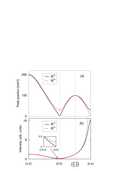
Figure 1: (Color online) (a)The $\delta$-function peak positions for $R^{zz}({\bf k},\omega)$ (solid line) and $R^{yy}({\bf k},\omega)$ (broken line) for ${\bf k}$ along symmetry lines. (b)Intensities of the peak for $R^{zz}({\bf k},\omega)$ and for $R^{yy}({\bf k},\omega)$. The gap mode at $(0,0)$ has a finite intensity as shown in Inset.

III Scattering operator of RIXS at the $L_{2,3}$ edge

III.1 Second-order optical process

The RIXS process is described by the electron-photon interaction Hamiltonian $H_{\textrm{int}}$. In the second-order optical process, the incident photon with wave vector $\textbf{q}_{i}$, energy $\omega_{i}$, and polarization $\alpha_{i}$ is absorbed by the material system, then the scattered photon with wave vector $\textbf{q}_{f}$, energy $\omega_{f}$, and polarization $\alpha_{f}$ is emitted. Then, the RIXS intensity $W(q_{f}\alpha_{f};q_{i}\alpha_{i})$ is written as,

$$W(q_{f}\alpha_{f};q_{i}\alpha_{i}) = 2\pi\sum_{f}\left|\sum_{n}\frac{\langle\Phi_{f}|H_{\rm int}|n\rangle\langle n|H_{\rm int}|\Phi_{i}\rangle}{E_{g}+\omega_{i}-E_{n}}\right|^{2}$$ (35)

$$\times \delta(E_{g}+\omega_{i}-E_{f}-\omega_{f}).$$

where $q_{i}\equiv({\bf q}_{i},\omega_{i})$ and $q_{f}\equiv({\bf q}_{f},\omega_{f})$. The initial and final states are given by $|\Phi_{i}\rangle=c_{q_{i}\alpha_{i}}^{\dagger}|g\rangle|0\rangle$ and $|\Phi_{f}\rangle=c_{q_{f}\alpha_{f}}^{\dagger}|f\rangle|0\rangle$, respectively, where $|g\rangle$ and $|f\rangle$ represent the ground and excited states of the matter with energies $E_{g}$ and $E_{f}$, respectively. The creation (annihilation) operator of the photon is denoted as $c_{\textbf{q}\alpha}^{\dagger}$ ($c_{\textbf{q}\alpha}$), which acts on the photon vacuum $|0\rangle$. The intermediate state $|n\rangle$ represents the eigenstate of the matter with energy $E_{n}$ in the presence of core hole.

At the Ir $L_{2,3}$ edge, $H_{\rm int}$ represents the electric dipole ($E$1) transition where a $2p$-core electron is excited to the $5d$ states. By restricting the transition within the manifold of $j_{\rm eff}=1/2$, it may be expressed as

$$H_{\rm int}=w\sum_{\textbf{q}}\frac{1}{\sqrt{2\omega_{\textbf{q}}}}\sum_{i,m,\sigma}D^{\alpha}(jm,\sigma)h_{i,\sigma}p_{i,jm}c_{\textbf{q}\alpha}{\rm e}^{i\textbf{q}\cdot\textbf{r}_{i}}+{\rm H.c.},$$ (36)

where $w$ is a constant proportional to $\int_{0}^{\infty}r^{3}R_{5d}(r)R_{2p}(r){\rm d}r$, with $R_{5d}(r)$ and $R_{2p}(r)$ being the radial wave-functions for the $5d$ and $2p$ states of Ir atom. The $p_{jm}$ ($p_{jm}^{\dagger}$) stands for the annihilation (creation) operator of the $2p$ core electron with the angular momentum $jm$, which states are defined in the local crystal coordinate frame. The operator $h_{i,\sigma}$ ($h_{i,\sigma}^{\dagger}$) represents the annihilation (creation) of 5d hole at site $i$ with the Kramers’ doublet specified by $\sigma$ ($=\uparrow$ or $\downarrow$) in hole picture, which quantization axis is rotated from the local crystal coordinate frame with Euler angles $\alpha$, $\beta$, and $\gamma$.Com (a) The coefficient $D^{\alpha}(jm,\sigma)$ describes the dependence on the $5d$ and core-hole states, which can be calculated in a similar manner as explained in Ref. Igarashi and Nagao, 2012 for cuprates.

III.2 Excitation and deexcitation of core hole at a single site

We analyze the situation that the core electron is excited and deexcited at the origin by following the procedure developed for undoped cuprates. The intermediate state just after the $E1$ transition takes place is given by

$$H_{\rm int}|g\rangle\propto\sum_{m}\left[\sum_{\sigma=\uparrow,\downarrow}D^{\alpha_{i}}(jm,\sigma)|\psi_{0}^{\sigma}\rangle\right]|jm\rangle.$$ (37)

Here we write $|g\rangle$ as

$$|g\rangle=|\uparrow\rangle|\psi_{0}^{\uparrow}\rangle+|\downarrow\rangle|\psi_{0}^{\downarrow}\rangle,$$ (38)

where $|\uparrow\rangle$ and $|\downarrow\rangle$ represent the normalized spin states at the origin, while $|\psi_{0}^{\uparrow}\rangle$ and $|\psi_{0}^{\downarrow}\rangle$ are constructed by the bases of the rest of spins, which are not normalized. The core hole state is represented as $|jm\rangle$. Note that the spin degrees of freedom of the $5d$ state is lost at the core-hole site, which is reminiscent of the introduction of non-magnetic impurity into spin system. Employing the normalized eigenstate $|\phi_{\eta}\rangle$’s with eigenvalue $\epsilon^{\prime}_{\eta}$ in the intermediate state, we have

$$|F\rangle \equiv \sum_{n}H_{\rm int}|n\rangle\frac{1}{\omega_{i}+E_{g}-E_{n}}\langle n|H_{\rm int}|\Phi_{i}\rangle$$ (39)

$$\propto \sum_{m,\sigma,\sigma^{\prime}}D^{\alpha_{f}}(jm,\sigma)^{*}D^{\alpha_{i}}(jm,\sigma^{\prime})$$

$$\times \sum_{\eta}|\sigma\rangle|\phi_{\eta}\rangle R(\epsilon^{\prime}_{\eta})\langle\phi_{\eta}|\psi_{0}^{\sigma^{\prime}}\rangle,$$

with

$$R(\epsilon^{\prime}_{\eta})=\frac{1}{\omega_{i}+\epsilon_{g}-\epsilon_{\rm core}+i\Gamma-\epsilon^{\prime}_{\eta}},$$ (40)

where $\epsilon_{g}$ and $\epsilon_{\rm core}$ denote the ground state energy of the magnetic system and the energy required to create a core hole in the state $|jm\rangle$ and the $5d^{6}$-configuration, respectively. The life-time broadening width of the core hole is denoted as $\Gamma$, which is around a few eV at the $L$ edge.Krause and Oliver (1979); Clancy et al. (2012) The first factor in the right hand side of Eq. (39) is rewritten as

$$\sum_{m}D^{\alpha_{f}}(jm,\sigma)^{*}D^{\alpha_{i}}(jm,\sigma) \equiv P_{\sigma}^{(0)}(j;\alpha_{f},\alpha_{i}),$$ (41)

$$\sum_{m}D^{\alpha_{f}}(jm,\sigma)^{*}D^{\alpha_{i}}(jm,-\sigma) \equiv P_{\sigma}^{(1)}(j;\alpha_{f},\alpha_{i}),$$ (42)

where $-\sigma$ denotes $\downarrow$ for $\sigma=\uparrow$ and vice versa. The $P_{\sigma}^{(0)}$ and $P_{\sigma}^{(1)}$ correspond to the spin-conserving and the spin-flip processes, respectively, whose values for $j=\frac{3}{2}$ are listed in Table 1 for $\alpha_{i}$ and $\alpha_{f}$ along the $x$, $y$, and $z$ axes. Note that they retain finite values even for the $z$ polarization, which contrasts with the case of the undoped cuprates where the $z$ polarization has no finite contribution.Igarashi and Nagao (2012) It can be confirmed that they vanish for $j=\frac{1}{2}$, consistent with the $L_{2}$ absorption experiment.Kim et al. (2009)

Table 1: $P_{\sigma}^{(0)}(\frac{3}{2};\alpha_{f},\alpha_{i})$ and $P_{\sigma}^{(1)}(\frac{3}{2};\alpha_{f},\alpha_{i})$ where upper and lower signs correspond to $\sigma=\uparrow$ and $\downarrow$, respectively.

		$P_{\sigma}^{(0)}$
$\alpha_{f}\setminus\alpha_{i}$	$x$	$y$	$z$
$x$	$\frac{2}{15}$	$\mp\frac{i}{15}\cos\beta$	$\pm\frac{i}{15}\sin\alpha\sin\beta$
$y$	$\pm\frac{i}{15}\cos\beta$	$\frac{2}{15}$	$\mp\frac{i}{15}\cos\alpha\sin\beta$
$z$	$\mp\frac{i}{15}\sin\alpha\sin\beta$	$\pm\frac{i}{15}\cos\alpha\sin\beta$	$\frac{2}{15}$
		$P_{\sigma}^{(1)}$
$x$	$0$	$\frac{i}{15}\sin\beta\textrm{e}^{\pm i\gamma}$	$\pm\frac{1}{15}[\cos\alpha\pm i\sin\alpha\cos\beta]\textrm{e}^{\pm i\gamma}$
$y$	$-\frac{i}{15}\sin\beta\textrm{e}^{\pm i\gamma}$	$0$	$-\frac{i}{15}[\cos\alpha\cos\beta\pm i\sin\alpha]\textrm{e}^{\pm i\gamma}$
$z$	$\mp\frac{1}{15}[\cos\alpha\pm i\sin\alpha\cos\beta]\textrm{e}^{\pm i\gamma}$	$\frac{i}{15}[\cos\alpha\cos\beta\pm i\sin\alpha]\textrm{e}^{\pm i\gamma}$	$0$

III.2.1 Spin-flipping channel

According to Eq. (39), the spin-flip process is given by

$$|F\rangle\propto\sum_{\sigma}P_{\sigma}^{(1)}|\sigma\rangle\sum_{\eta}|\phi_{\eta}\rangle R(\epsilon^{\prime}_{\eta})\langle\phi_{\eta}|\psi_{0}^{-\sigma}\rangle$$ (43)

We expand $|F\rangle$ by $S_{0}^{-}|g\rangle$ and $S_{0}^{+}|g\rangle$ with neglecting excitations outside the core-hole site ($S_{0}^{\pm}\equiv S_{0}^{x^{\prime}}\pm iS_{0}^{y^{\prime}}$). Note that they are orthogonal to each other and to $|g\rangle$, but not normalized, that is, $\langle g|S_{0}^{-}S_{0}^{+}|g\rangle=\langle\psi_{0}^{\downarrow}|\psi_{0}^{\downarrow}\rangle$ and $\langle g|S_{0}^{+}S_{0}^{-}|g\rangle=\langle\psi_{0}^{\uparrow}|\psi_{0}^{\uparrow}\rangle$. Therefore, introducing the quantity

$$f_{\sigma}^{(1)}(\omega_{i})=\frac{1}{\langle\psi_{0}^{\sigma}|\psi_{0}^{\sigma}\rangle}\langle\psi_{0}^{\sigma}|\sum_{\eta}|\phi_{\eta}\rangle R(\epsilon_{\eta}^{\prime})\langle\phi_{\eta}|\psi_{0}^{\sigma}\rangle,$$ (44)

we have

$$|F\rangle\sim P_{\downarrow}^{(1)}f_{\uparrow}^{(1)}(\omega_{i})S_{0}^{-}|g\rangle+P_{\uparrow}^{(1)}f_{\downarrow}^{(1)}(\omega_{i})S_{0}^{+}|g\rangle.$$ (45)

Since the process for $\sigma=\uparrow$ is generally different from that for $\sigma=\downarrow$ in the antiferromagnetic state, $f_{\sigma}^{(1)}(\omega_{i})$ may be written as

$$f_{\sigma}^{(1)}(\omega_{i})=f_{0}^{(1)}(\omega_{i})\pm\frac{1}{2}\Delta(\omega_{i}),$$ (46)

where plus and minus signs in the second term correspond to $\sigma=\uparrow$ and $\downarrow$, respectively. The $\Delta(\omega_{i})$, which is expressed as $f_{\uparrow}^{(1)}(\omega_{i})-f_{\downarrow}^{(1)}(\omega_{i})$, is proportional to the sublattice magnetization when it is small, since it vanishes without the antiferromagnetic long-range order. Inserting Eq. (46) into Eq. (45), we obtain the final expression. For example, we have for $\alpha_{f}$ along the $x$ axis and $\alpha_{i}$ along the $z$ axis,

$$|F\rangle \propto \left(\frac{2}{15}\right)if^{(1)}(\omega_{i})\left[M_{12}S_{0}^{x^{\prime}}+M_{22}S_{0}^{y^{\prime}}\right]$$ (47)

$$+ \frac{1}{15}\Delta(\omega_{i})\left[M_{12}S_{0}^{y^{\prime}}-M_{22}S_{0}^{x^{\prime}}\right],$$

where $M_{ij}$ stands for the $(i,j)$ component of the conventional rotation matrix with the Euler angles $(\alpha,\beta,\gamma)$.Com (b) A full consideration over the polarizations leads to

$$|F\rangle \propto \left(-\frac{2}{15}\right)if_{0}^{(1)}(\omega_{i})(\mbox{\boldmath{$\alpha$}}_{f}\times\mbox{\boldmath{$\alpha$}}_{i})\cdot{\bf S}_{0\perp}|g\rangle$$ (48)

$$- \left(-\frac{1}{15}\right)\Delta(\omega_{i})(\mbox{\boldmath{$\alpha$}}_{f}\times\mbox{\boldmath{$\alpha$}}_{i})\cdot({\bf e}_{m}\times{\bf S}_{0})|g\rangle,$$

where ${\bf S}_{0\perp}$ represents the component perpendicular to the direction of the staggered magnetic moment, and $\rm{\bf e}_{m}$ represents the unit vector along the direction of the sublattice magnetization.

III.2.2 Spin-conserving channel

According to Eq. (39), the spin-conserving process is given by

$$|F\rangle\propto\sum_{\sigma}P_{\sigma}^{(0)}|\sigma\rangle\sum_{\eta}|\phi_{\eta}\rangle R(\epsilon^{\prime}_{\eta})\langle\phi_{\eta}|\psi_{0}^{\sigma}\rangle.$$ (49)

We expand $|F\rangle$ by $|g\rangle$ and $S_{0}^{z^{\prime}}|g\rangle$ by neglecting the excitations outside the core-hole site. Note that $S_{0}^{z^{\prime}}|g\rangle$ is not orthogonal to $|g\rangle$ nor normalized. Let $|\psi_{1}\rangle$ and $|\psi_{2}\rangle$ be $|g\rangle$ and $S_{0}^{z^{\prime}}|g\rangle$, respectively. Then the overlap matrix $[\hat{\rho}]_{i,j}\equiv\langle\psi_{i}|\psi_{j}\rangle$ is given by

$$\hat{\rho}=\left(\begin{array}[]{cc}1&\langle S_{0}^{z^{\prime}}\rangle\\ \langle S_{0}^{z^{\prime}}\rangle&\frac{1}{4}\end{array}\right).$$ (50)

We project onto these states by operating $\sum_{i,j}|\psi_{i}\rangle(\hat{\rho}^{-1})_{i,j}\langle\psi_{j}|$. For the channel preserving the direction of the polarization during the scattering process, we have

$$|F\rangle\propto\left(\frac{2}{15}\right)(\mbox{\boldmath{$\alpha$}}_{f}\cdot\mbox{\boldmath{$\alpha$}}_{i})\left[f_{0}(\omega_{i})|g\rangle+\Delta(\omega_{i}){\bf e}_{m}\cdot{\bf S}_{0}|g\rangle\right].$$ (51)

Similarly, for the scattering channel changing the direction of the polarization during the process, by using $P_{\uparrow}^{(0)}=-P_{\downarrow}^{(0)}$, we obtain

$$|F\rangle \propto \left(-\frac{1}{15}\right)i\frac{1}{2}\Delta(\omega_{i})(\mbox{\boldmath{$\alpha$}}_{f}\times\mbox{\boldmath{$\alpha$}}_{i})\cdot{\bf e}_{m}|g\rangle$$ (52)

$$+ \left(-\frac{2}{15}\right)if_{0}^{(1)}(\omega_{i})(\mbox{\boldmath{$\alpha$}}_{f}\times\mbox{\boldmath{$\alpha$}}_{i})\cdot{\bf S}_{0\parallel}|g\rangle,$$

where ${\bf S}_{0\parallel}$ represents the component parallel to the direction of the staggered magnetic moment.

III.2.3 Elastic scattering

The amplitude of elastic scattering is given by $\langle g|F\rangle$. The first term of Eq. (51) gives a contribution independent of the magnetic order, while the second term of Eq. (51) gives a contribution proportional to $|{\bf m}|^{2}$, since $\Delta(\omega_{i})$ is proportional to $|{\bf m}|$. Here ${\bf m}$ stands for the sublattice magnetization. Both terms in Eq. (52) give the contributions proportional to $(\mbox{\boldmath{$\alpha$}}_{f}\times\mbox{\boldmath{$\alpha$}}_{i})\cdot{\bf m}$, which is consistent with the formula given by Hannon et. al. Hannon et al. (1988)

III.2.4 Remarks

Here, it is interesting to compare our result derived on the basis of the projection method with other well-known results; one is the far-off-resonance condition that $|\omega_{i}-\epsilon_{\rm core}|\gg|\epsilon^{\prime}_{\eta}-\epsilon_{g}|$, and another is the large limit of $\Gamma$, which is called as the fast collision approximation (FCA). Ament et al. (2007, 2009); Haverkort (2010) In both latter conditions, we could factor out $R(\epsilon^{\prime}_{\eta})$ from the summation over $\eta$ in Eq. (44). Then, using the closure relation of $|\phi_{\eta}\rangle$, we immediately obtain $\Delta(\omega_{i})=0$. The presence of $\Delta(\omega_{i})$ is a hallmark of a second-order process that the x ray could recognize the long-range order in the scattering process, contrast with neutron scattering. In the present case, however, $\Delta(\omega_{i})$ is estimated to be quite small, since the life-time broadening width is rather large at the Ir L-edge.Krause and Oliver (1979) By neglecting $\Delta(\omega_{i})$, Eqs. (48) and (52) are summarized into an expression, which is similar to that for the undoped cuprates, Ament et al. (2007, 2009); Haverkort (2010); Igarashi and Nagao (2012); Com (c) as

$$|F\rangle\propto\left(-\frac{2}{15}\right)if_{0}^{(1)}(\omega_{i})(\mbox{\boldmath{$\alpha$}}_{f}\times\mbox{\boldmath{$\alpha$}}_{i})\cdot{\bf S}_{0}|g\rangle.$$ (53)

Note that when both $f_{0}^{(1)}(\omega_{i})$ and $\Delta(\omega_{i})$ are numerically relevant, their $\omega_{i}$ dependence might be a intriguing feature. However, once $\Delta(\omega_{i})$ is neglected as in the present case, we do not have to evaluate the value of $f_{0}^{(1)}(\omega_{i})$, since RIXS cannot tell about the absolute magnitude of the intensity.

IV Analysis of RIXS spectra from Sr₂IrO₄

We consider the specific case of a 90^∘ scattering angle. The scattering plane is perpendicular to the IrO₂ plane and intersects the $ab$ plane with the $[110]$ direction, as illustrated in Fig. 2(a). The incident x ray is assumed to have the $\pi$ polarization. Since $\omega\sim 11.2$ keV and $|{\bf q}_{i}|\sim 5.7$ $\textrm{\AA}^{-1}$ at the Ir $L_{3}$ edge, only a few degrees of tilt of the scattering plane could sweep the entire Brillouin zone.

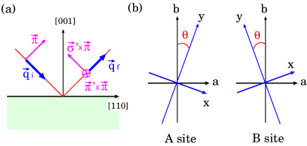
Figure 2: (Color online) (a) Geometry of 90^∘ scattering. The scattering plane is perpendicular to the $ab$ plane and intersects the $ab$ plane with the $[110]$ direction. (b) Local coordinate frames of the two sublattices, which are rotated by angle $\pm\theta$ around the $c$ axis.

The scattering operator $Z^{(1)}({\bf q})$ is given by summing up the amplitude with multiplying $\exp(i{\bf q}\cdot{\bf r}_{j})$ at each Ir site ${\bf r}_{j}$,

$$Z^{(1)}({\bf q})\equiv\frac{1}{\sqrt{N}}\sum_{j}(\mbox{\boldmath{$\alpha$}}_{f}\times\mbox{\boldmath{$\alpha$}}_{i})\cdot{\bf S}_{j}{\rm e}^{-i\textbf{q}\cdot\textbf{r}_{j}},$$ (54)

where ${\bf q}\equiv{\bf q}_{i}-{\bf q}_{f}$ is the momentum transfer. Note that the local coordinate frames defining spin operators are different between the A and B sites, as illustrated in Fig. 2(b). Evaluating $\mbox{\boldmath{$\alpha$}}_{f}\times\mbox{\boldmath{$\alpha$}}_{i}$ in the local coordinate frame, we have $Z^{(1}({\bf q})$ for ${\bf q}$ inside the first MBZ,

$$Z^{(1)}({\bf q}) = -\frac{1}{2}\left[\cos\theta\,Q_{+}^{x}({\bf q})-\sin\theta\,Q_{-}^{x}({\bf q})\right.$$ (55)

$$\left.+\cos\theta\,Q_{+}^{y}({\bf q})+\sin\theta\,Q_{-}^{y}({\bf q})\right]+\frac{1}{\sqrt{2}}Q_{+}^{z}({\bf q}),$$

in the $\sigma^{\prime}\times\pi$ channel, and

$$Z^{(1)}({\bf q}) = -\frac{1}{\sqrt{2}}\left[\cos\theta\,Q_{+}^{x}({\bf q})+\sin\theta\,Q_{-}^{x}({\bf q})\right.$$ (56)

$$\left.-\cos\theta\,Q_{+}^{y}({\bf q})+\sin\theta\,Q_{-}^{y}({\bf q})\right].$$

in the $\pi^{\prime}\times\pi$ channel. The scattering operators for ${\bf q}$ outside the first MBZ are given by replacing $Q_{\pm}^{\mu}({\bf q})$ with $Q_{\mp}^{\mu}([{\bf q}])$.

The RIXS intensity is proportional to the correlation functions for these scattering operators,

$$I\equiv W(q_{f}\alpha_{f};q_{i}\alpha_{i})\propto\int_{-\infty}^{\infty}\langle Z^{(1)}({\bf q},t)Z^{(1)}(-{\bf q},0)\rangle{\rm e}^{i\omega t}{\rm d}t.$$ (57)

The insertion of Eqs. (55) and (56) into Eq. (57) leads to the expression for ${\bf q}$ inside the first MBZ

$$I\propto\left\{\begin{array}[]{ll}\frac{\cos^{2}\theta\,R_{+}^{yy}({\bf q},\omega)+\sin^{2}\theta\,R_{-}^{yy}({\bf q},\omega)+2R_{+}^{zz}({\bf q},\omega)}{4},&{\rm for}\ \sigma^{\prime}\times\pi,\\ \frac{\cos^{2}\theta\,R_{+}^{yy}({\bf q},\omega)+\sin^{2}\theta\,R_{-}^{yy}({\bf q},\omega)}{2},&{\rm for}\ \pi^{\prime}\times\pi,\end{array}\right..$$ (58)

We have neglected $R_{\pm}^{xx}({\bf q},\omega)$, since it is a higher order of $1/S$. To extend the expression to outside the first MBZ, $R_{+}^{yy}({\bf q},\omega)$, $R_{+}^{zz}({\bf q},\omega)$ and $R_{-}^{yy}({\bf q},\omega)$ are replaced by $R_{-}^{yy}([{\bf q}],\omega)$ and $R_{-}^{zz}([{\bf q}],\omega)$ and $R_{+}^{yy}([{\bf q}],\omega)$, respectively. Note that the $\sin^{2}\theta$-terms give the antibonding contribution for ${\bf q}$ inside the first MBZ, which diverges at $\omega=0$ with ${\bf q}\to(0,0)$. This unusual contribution may be interpreted as a reflection of the weak ferromagnetism.

Figure 3 shows the numerical results with the same parameter values as for the correlation function. Panel (a) shows the RIXS spectra as a function of $\omega$ for ${\bf q}$ along the symmetry lines, and panel (b) shows the intensities of two peaks. The intensities from the $\sigma^{\prime}$ and $\pi^{\prime}$ polarization channels are summed up. At ${\bf q}=(0,0)$, the intensity of the peak diverges at $\omega=0$ due to the weak ferromagnetism ($\sin^{2}\theta$-term), while that of another peak is quite small at $\omega=29$ meV. The effect of the weak ferromagnetism is limited very close to the $\Gamma$ point. At ${\bf q}=(\pi,\pi)$, the intensity of the peak also diverges at $\omega=0$ due to the antiferromagnetic order, while that of another peak is rather large at $\omega=29$ meV.

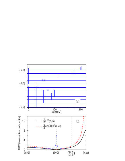
Figure 3: (Color online) (a) RIXS spectra as a function of $\omega$ for ${\bf q}$ along symmetry lines evaluated for $\theta=\pm 11^{\circ}$. Vertical bars represent the $\delta$-function peaks with heights proportional to their intensities. The height for the peaks at $\omega=0$ is divergent, and are cut to be finite on the figure. (b) Peak intensities of $\frac{1}{2}R^{zz}({\bf q},\omega)$ (black solid line) and $\frac{3}{4}\cos^{2}\theta R^{yy}({\bf q},\omega)$ (red broken line) for $\theta=0$. The (blue) broken-dotted line shows the intensity added by the $\sin^{2}\theta$ terms for $\theta=\pm 11^{\circ}$, which makes the curve deviate from the curve at $\theta=0$ for ${\bf q}$ only close to $(0,0)$.

V Concluding remarks

We have studied the magnetic excitations in Sr₂IrO₄ on the basis of the Heisenberg model with isotropic exchange couplings and small anisotropic terms. Solving the coupled equations of motion for the Green’s functions within the spin-wave approximation, we have found that two modes emerge with slightly different energies. Introducing the bonding and antibonding combinations of spin operators at A and B sites, we have considered the correlation functions for these operators. We have found that the correlation functions with the $y$ and $z$ spin-components are composed of a single $\delta$-function peak with different energies corresponding to each mode. We have analyzed the second-order RIXS process with the assumption that the excitations are confined on the core-hole site, and have obtained the expression for the local scattering operator composed of the term consistent with the FCA as well as a term existing only in the broken symmetric phase. The latter is, however, expected to be quite small in Sr₂IrO₄, since the life-time broadening width at the $L$ edge of Ir is rather large. Using the scattering operator, the RIXS intensity has been expressed by a sum of the correlation functions with two spin components. Having evaluated the formula, we have demonstrated that the spectra are composed of two peaks originated from the split modes. Such two-peak structures have not been observed in the RIXS experiments. Kim et al. (2012b); Ament et al. (2011) We hope that the present analysis may help to verify the mode splitting in the experiments with improving the instrumental energy resolution. Sala et al. (2013)

Here, we comment on the effect of $\Delta(\omega_{i})$ on the RIXS spectrum, which becomes relevant when the core-hole lifetime broadening $\Gamma$ is small. It then requires a reliable evaluation of the coefficients $f_{0}^{(1)}(\omega_{i})$ and $\Delta(\omega_{i})$ to calculate the RIXS intensity. In our previous work, we have confirmed that analysis utilizing a small cluster works well in evaluating the coefficients with moderate accuracy for cuprates, which have revealed that the RIXS intensity showed a characteristic q-dependence for small $\Gamma$.Igarashi and Nagao (2012) However, such evaluation for the present case is very difficult because the magnitude of the exchange coupling between the third neighbors remains significant in Sr₂IrO₄, which requires an analysis for a larger cluster. An analysis with high accuracy in this direction will be an intriguing future work.

The present study is based on the localized electron picture, which works well on the magnetic excitations in the strong coupling limit. Anderson (1959) However, other peak structures have been observed around the region of $0.4\sim 0.6$ eV in the RIXS experiment, which could be attributed to the excitations from $j_{\textrm{eff}}=1/2$ to $3/2$ multiplets.Kim et al. (2012b); Ament et al. (2011) Since the Mott-Hubbard gap is estimated as $\sim 0.4$ eV from the optical absorption spectra,Kim et al. (2008); Moon et al. (2009) this energy region also coincides with the energy continuum of the electron-hole pair creation. In such a situation, it may make sense to consider the spectra from the itinerant electron picture in order to obtain a coherent picture of RIXS spectra. Such study based on the Hartree-Fock and RPA approximations is under progress.Igarashi and Nagao (2013b)

Appendix A Symmetry relations among the Green’s functions

We consider the Green’s function defined by

$$G_{AB}(\omega)=-i\int\langle T[A(t)B(0)]\rangle{\rm e}^{i\omega t}{\rm d}t,$$ (59)

where $A$ and $B$ are boson operators. It is expressed in the spectral representation as

$$G_{AB}(\omega)=\sum_{n}\left\{\frac{\langle g|A|n\rangle\langle n|B|g\rangle}{\omega-E_{n}+E_{g}+i\delta}-\frac{\langle g|B|n\rangle\langle n|A|g\rangle}{\omega+E_{n}-E_{g}-i\delta}\right\},$$ (60)

where $|n\rangle$ stands for the eigenstate of the Hamiltonian with energy $E_{n}$, and $|g\rangle$ the ground state with energy $E_{g}$. It is easily proved from this expression that

$$G_{B^{\dagger}A^{\dagger}}(\omega)=G_{AB}(\omega),\quad G_{A^{\dagger}B^{\dagger}}(\omega)=G_{AB}(-\omega).$$ (61)

Hence we obtain the relations between the Green’s functions of Holstein-Primakoff bosons by replacing A by one of $a({\bf k})$, $a^{\dagger}({-\bf k})$, $b({\bf k})$, $b^{\dagger}({-\bf k})$, and B by one of $a(-{\bf k})$, $a^{\dagger}({\bf k})$, $b(-{\bf k})$, $b^{\dagger}({\bf k})$. In addition, since the Hamiltonian is invariant with exchanging $a$ and $b$ as well as $a^{\dagger}$ and $b^{\dagger}$, the Green’s functions remain the same forms by such exchange.

References

• Crawford et al. (1994) M. K. Crawford, M. A. Subramanian, R. L. Harlow, J. A. Fernandez-Baca, Z. R. Wang, and D. C. Johnston, Phys. Rev. B 49, 9198 (1994).
• Cao et al. (1998) G. Cao, J. Bolivar, S. McCall, J. E. Crow, and R. P. Guertin, Phys. Rev. B 57, R11039 (1998).
• Moon et al. (2006) S. J. Moon, M. W. Kim, K. W. Kim, Y. S. Lee, J.-Y. Kim, J.-H. Park, B. J. Kim, S.-J. Oh, S. Nakatsuji, Y. Maeno, et al., Phys. Rev. B 74, 113104 (2006).
• Clancy et al. (2012) J. P. Clancy, N. Chen, C. Y. Kim, W. F. Chen, K. W. Plumb, B. C. Jeon, T. W. Noh, and Y.-J. Kim, Phys. Rev. B 86, 195131 (2012).
• Ye et al. (2013) F. Ye, S. Chi, B. C. Chakoumakos, J. A. Fernandez-Baca, T. Qi, and G. Cao, Phys. Rev. B 87, 140406 (R) (2013).
• Dhital et al. (2013) C. Dhital, T. Hogan, Z. Yamani, C. de la Cruz, X. Chen, S. Khadka, Z. Ren, and S. D. Wilson, Phys. Rev. B 87, 144405 (2013).
• Kim et al. (2008) B. J. Kim, H. Jin, S. J. Moon, J.-Y. Kim, B.-G. Park, C. S. Leem, J. Yu, T. W. Noh, C. Kim, S.-J. Oh, et al., Phys. Rev. Lett. 101, 076402 (2008).
• Arita et al. (2012) R. Arita, J. Kuneš, A. V. Kozhevnikov, A. G. Eguiluz, and M. Imada, Phys. Rev. Lett. 108, 086403 (2012).
• Watanabe et al. (2010) H. Watanabe, T. Shirakawa, and S. Yunoki, Phys. Rev. Lett. 105, 216410 (2010).
• Kim et al. (2009) B. J. Kim, H. Ohsumi, T. Komesu, S. Sakai, T. Morita, H. Takagi, and T. Arima, Science 323, 1329 (2009).
• Anderson (1959) P. W. Anderson, Phys. Rev. 115, 2 (1959).
• Jackeli and Khaliullin (2009) G. Jackeli and G. Khaliullin, Phys. Rev. Lett. 102, 017205 (2009).
• Jin et al. (2009) H. Jin, H. Jeong, T. Ozaki, and J. Yu, Phys. Rev. B 80, 075112 (2009).
• Kim et al. (2012a) B. H. Kim, G. Khaliullin, and B. I. Min, Phys. Rev. Lett. 109, 167205 (2012a).
• Wang and Senthil (2011) F. Wang and T. Senthil, Phys. Rev. Lett. 106, 136402 (2011).
• Holstein and Primakoff (1940) T. Holstein and H. Primakoff, Phys. Rev. 58, 1098 (1940).
• Igarashi and Nagao (2013a) J. I. Igarashi and T. Nagao, Phys. Rev. B 88, 104406 (2013a).
• Bulut et al. (1989) N. Bulut, D. Hone, D. J. Scalapino, and E. Y. Loh, Phys. Rev. Lett. 62, 2192 (1989).
• Braicovich et al. (2009) L. Braicovich, L. J. P. Ament, V. Bisogni, F. Forte, C. Aruta, G. Balestrino, N. B. Brookes, G. M. De Luca, P. G. Medaglia, F. M. Granozio, et al., Phys. Rev. Lett. 102, 167401 (2009).
• Braicovich et al. (2010) L. Braicovich, J. van den Brink, V. Bisogni, M. M. Sala, L. J. P. Ament, N. B. Brookes, G. M. De Luca, M. Salluzzo, T. Schmitt, V. N. Strocov, et al., Phys. Rev. Lett. 104, 077002 (2010).
• Guarise et al. (2010) M. Guarise, B. D. Piazza, M. M. Sala, G. Ghiringhelli, L. Braicovich, H. Berger, J. N. Hancock, D. van der Marel, T. Schmitt, V. N. Strocov, et al., Phys. Rev. Lett. 105, 157006 (2010).
• Ishii et al. (2011) K. Ishii, I. Jarrige, M. Yoshida, K. Ikeuchi, J. Mizuki, K. Ohashi, T. Takayama, J. Matsuno, and H. Takagi, Phys. Rev. B 83, 115121 (2011).
• Kim et al. (2012b) J. Kim, D. Casa, M. H. Upton, T. Gog, Y.-J. Kim, J. F. Mitchell, M. van Veenendaal, M. Daghofer, J. van den Brink, G. Khaliullin, et al., Phys. Rev. Lett. 108, 177003 (2012b).
• Ament et al. (2011) L. J. P. Ament, G. Khaliullin, and J. van den Brink, Phys. Rev. B 84, 020403 (R) (2011).
• Igarashi and Nagao (2012) J. I. Igarashi and T. Nagao, Phys. Rev. B 85, 064421 (2012).
• Ament et al. (2007) L. J. P. Ament, F. Forte, and J. van den Brink, Phys. Rev. B 75, 115118 (2007).
• Ament et al. (2009) L. J. P. Ament, G. Ghiringhelli, M. M. Sala, L. Braicovich, and J. van den Brink, Phys. Rev. Lett. 103, 117003 (2009).
• Haverkort (2010) M. W. Haverkort, Phys. Rev. Lett. 105, 167404 (2010).
• Kanamori (1957) J. Kanamori, Prog. Theor. Phys. 17, 177 (1957).
• Com (a) In the $j_{\rm eff}=\frac{1}{2}$ manifold, $h_{\uparrow}^{\dagger}$ and $h_{\downarrow}^{\dagger}$ are defined by $h_{\uparrow}^{\dagger}|{\rm vac}\rangle=d_{\downarrow}|0\rangle$, $h_{\downarrow}^{\dagger}|{\rm vac}\rangle=-d_{\uparrow}|0\rangle$, with $|{\rm vac}\rangle=d_{\uparrow}^{\dagger}d_{\downarrow}^{\dagger}|0\rangle$, where $d_{\sigma}$ is the annihilation operator of electron with the Kramers’ doublet specified by $\sigma$.
• Krause and Oliver (1979) M. O. Krause and J. H. Oliver, J. Phys. Chem. Ref. Data 8, 329 (1979).
• Com (b) See, for example, Eq. (4.43) in R. E. Rose, Elementary Theory of Angular Momentum (Wiley, New York, 1957).
• Hannon et al. (1988) J. P. Hannon, G. T. Trammell, M. Blume, and D. Gibbs, Phys. Rev. Lett. 61, 1245 (1988).
• Com (c) For undoped cuprates, $\alpha_{i}$ and $\alpha_{f}$ in Eq. (53) are replaced by those projected onto the $ab$ plane.
• Sala et al. (2013) M. M. Sala, C. Henriquet, L. Simonelli, R. Verbeni, and G. Monaco, J. Electron Spectrosc. Relat. Phenom. 188, 150 (2013).
• Moon et al. (2009) S. J. Moon, H. Jin, W. S. Choi, J. S. Lee, S. S. A. Seo, J. Yu, G. Cao, T. W. Noh, and Y. S. Lee, Phys. Rev. B 80, 195110 (2009).
• Igarashi and Nagao (2013b) J. I. Igarashi and T. Nagao, Phys. Rev. B 88, 014407 (2013b).