Far-Infrared Extinction Mapping of Infrared Dark Clouds

Abstract

Progress in understanding star formation requires detailed observational constraints on the initial conditions, i.e. dense clumps and cores in giant molecular clouds that are on the verge of gravitational instability. Such structures have been studied by their extinction of Near-Infrared (NIR) and, more recently, Mid-Infrared (MIR) background light. It has been somewhat more of a surprise to find that there are regions that appear as dark shadows at Far-Infrared (FIR) wavelengths as long as $\sim 100\micron$! Here we develop analysis methods of FIR images from Spitzer-MIPS and Herschel-PACS that allow quantitative measurements of cloud mass surface density, $\Sigma$. The method builds upon that developed for MIR extinction mapping (MIREX) (Butler & Tan, 2012), in particular involving a search for independent saturated, i.e. very opaque, regions that allow measurement of the foreground intensity. We focus on three massive starless core/clumps in IRDC G028.37+00.07, deriving mass surface density maps from 3.5 to $70\>\micron$. A by-product of this analysis is measurement of the spectral energy distribution of the diffuse foreground emission. The lower opacity at $70\>\micron$ allows us to probe to higher $\Sigma$ values, up to $\sim 1\>{\rm{g\>cm}^{-2}}$ in the densest parts of the core/clumps. Comparison of the $\Sigma$ maps at different wavelengths constrains the shape of the MIR-FIR dust opacity law in IRDCs. We find it is most consistent with the thick ice mantle models of Ossenkopf & Henning (1994). There is tentative evidence for grain ice mantle growth as one goes from lower to higher $\Sigma$ regions.

1. Introduction

The molecular gas clumps that form star clusters are important links between the large, Galactic-scale and small, individual-star-scale processes of star formation. Most stars are thought to form from these structures (e.g., Lada & Lada, 2003; Gutermuth et al., 2009). Massive stars may form from massive starless cores buried in such clumps (e.g., Mckee & Tan, 2003).

Observations of clumps in their earliest stages of star formation are thus important for constraining theoretical models of massive star and star cluster formation. These early-stage clumps are expected to be cold and dense, and large populations have been revealed as “Infrared Dark Clouds” (IRDCs) via their absorption of the diffuse MIR ($\sim 10\>\micron$) emission of the Galactic interstellar medium (e.g. Egan et al. 1998; Simon et al. 2006 [S06]; Peretto et al. 2009; Butler & Tan 2009). With the advent of longer wavelength imaging data from Spitzer-MIPS (Carey et al., 2009) and Herschel-PACS (e.g., Peretto et al., 2010; Henning et al., 2010), some IRDCs are appear dark at wavelengths up to $\sim 100\>\micron$.

Butler & Tan (2009, 2012 [BT09, BT12]) developed MIR extinction (MIREX) mapping with Spitzer-IRAC 8$\micron$ GLIMPSE survey data (Churchwell et al., 2009). Using this method, which does not require knowledge of cloud temperature, they derived mass surface density, $\Sigma$, maps of 10 IRDCs with angular resolution of 2$\arcsec$. The maps probed $\Sigma$ up to $\sim 0.5\>{\rm{g\>cm}}^{-2}$ ($A_{V}\sim 100\>{\rm{mag}}$), with this limit set by the image noise level and the adopted opacity of $7.5\>{\rm{cm^{2}\>g^{-1}}}$ (based on thin ice mantle dust models; Ossenkopf & Henning (1994) [OH94]).

However, higher $\Sigma$ clouds have been claimed based on FIR/mm dust emission (e.g., Battersby et al., 2011; Ragan et al., 2012), although this requires also estimating the dust temperature. Some already-formed star clusters have cores with $\Sigma>1\>{\rm{g\>cm}}^{-2}$ (e.g., Tan et al., 2013a). It is thus important to see if extinction mapping methods can be developed that can probe to higher $\Sigma$ values. Butler, Tan & Kainulainen (2013 [BTK]) have attempted this by using more sensitive (longer exposure) 8 $\micron$ images. Here we develop methods that probe to higher $\Sigma$ via FIR extinction mapping using Spitzer-MIPS 24 and Herschel-PACS 70$\micron$ images with 6″ angular resolution. At these wavelengths, IRDCs still appear dark but have smaller optical depths. Our method also requires us to examine the FIR extinction law and its possible variations within dense gas, which may be caused by grain coagulation and ice mantle formation.

2. The Far-Infrared Extinction (FIREX) Mapping Method

2.1. MIR and FIR Imaging Data for IRDC G028.37+00.07

We utilize Spitzer-MIPS $24\micron$ images from the MIPSGAL survey (Carey et al., 2009) that have 6″ resolution and estimated $1\sigma$ noise level of $0.25\>$MJy/sr.

We also analyze archival $70\micron$ Herschel-PACS images. The first type (proposal ID KPGT-okrause-1) were observed with medium scanning speed and also have $\simeq$6″ resolution, but do not cover a very large area around the IRDC ($\sim 16$′ in extent). We estimate a $1\sigma$ noise level of $\sim 15\>$MJy/sr, i.e. about a factor of two better than achieved with fast scanning observations (Traficante et al., 2011). The second type (proposal ID KPOT-smolinar-1) were observed in the Galactic plane HiGAL survey (Molinari et al., 2010) in fast scanning mode with $\sim$9″ resolution. These data are useful for assessing intensity of the Galactic background emission, which needs to be interpolated from regions surrounding the IRDC.

Both the Herschel data sets are obtained already processed to level 2.5 in HIPE, so zero-level offsets need to be applied to have measurements of absolute values of specific intensities. We adopted a model spectral energy distribution (SED) of the diffuse Galactic plane emission (Li & Draine 2001 [LD01]) from NIR to FIR. We fit this model to the observed median intensities in a 2$\arcdeg\times$2$\arcdeg$ field centered on the cloud, considering data at 8$\micron$ (Spitzer-IRAC), 24$\micron$ (Spitzer-MIPS), 60$\micron$ and 100$\micron$ (both IRAS) and then predicted the expect intensities in the Herschel-PACS 70µm band. A single offset value was then applied to each Herschel dataset (908 MJy/sr and 241 MJy/sr for medium and fast scan data, respectively). We tested this method against offset corrections reported by Bernard et al. (2010) at $l=30\arcdeg$ based on Planck data, finding agreement at the $\simeq 10\%$ level.

We find an astrometric difference of a few arcseconds between the Herschel and Spitzer maps. We corrected this by the average value of the mean positional offset of four point sources seen at 8, 24 and 70 $\rm{\mu}m$, amounting to a 3.4″ translation at P.A. 62.7$\arcdeg$. The resulting three-color image of the IRDC is shown in Fig. 1.

While our focus is on FIR data, we also compare to Spitzer-IRAC 3.5, 4.5, 5.9, $8\micron$ (GLIMPSE) images, which have 2″ resolution at 8µm. For these, we adopt $1\sigma$ noise levels of 0.3 MJy/sr, 0.3 MJy/sr, 0.7 MJy/sr, 0.6 MJy/sr, respectively (Reach et al., 2006).

To compare multiwavelength extinction mapping pixel by pixel, we regrid the IRAC images to the 24µm MIPS frame with its $1.25\arcsec\times 1.25\arcsec$ pixels, similar to the 1.2″ IRAC pixels. However, for Herschel-PACS data, with its 3.2″ pixels, we first carry out extinction mapping on the original pixel grid (especially searching for saturated pixels, see below), before finally regridding to the MIPS frame for multiwavelength comparison.

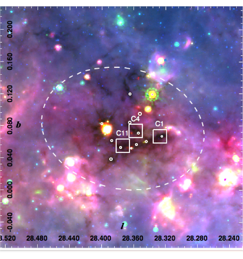
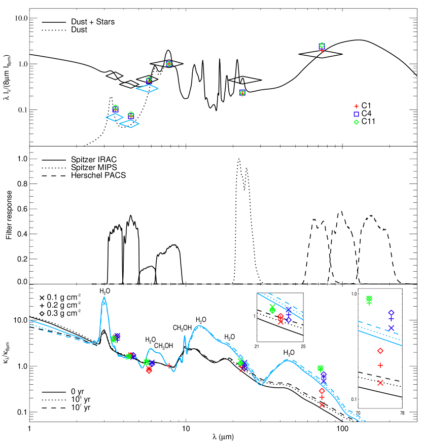
Figure 1.— (a) Left: Three-color image of IRDC G028.37+00.07 (red: 70$\micron$, green: 24$\micron$ & blue: 8$\micron$). Small circles indicate massive cores studied by BT12 and BTK. Squares are regions inspected for local saturation around cores C1, C4 & C11. Dashed ellipse shows the IRDC boundary from S06. (b) Right top: Total IR to sub-mm SED (solid line) of the Galactic plane in the “MIRS” region at $l\simeq 44\arcdeg$ (LD01). Dotted line shows contribution to this from dust; stars dominate at short wavelengths. Large diamonds indicate convolution of these SEDs with the filter response function of corresponding instruments (panel (b)). The red/blue/green symbols show foreground intensities, relative to the LD01 IRAC 8$\micron$ value, measured to the three saturated cores C1/C4/C11, respectively. (c) Right middle: Filter response of IRAC bands 1-4 (solid lines), MIPS 24$\micron$ (dotted line) and PACS 70, 100, & 160$\micron$ (dashed lines). (d) Right bottom: Dust opacities relative to effective opacity measured in the IRAC 8$\micron$ band. Black/blue lines show thin/thick ice mantle models of OH94. Solid lines show the initial, uncoagulated MRN grain population. Dotted and dashed lines indicate these models after $10^{5}$ and $10^{7}\>{\rm{yr}}$ of coagulation at $n_{\rm{H}}=10^{6}\>{\rm{cm}}^{-3}$, respectively. The red/blue/green symbols (for C1/C4/C11 regions; slight wavelength offsets applied for clarity) show $\kappa_{\lambda}/\kappa_{8\micron}$ for the indicated $\Sigma$ ranges.

2.2. Radiative Transfer and Foreground Estimation

We adopt the 1D radiative transfer model of BT12, which requires knowing the intensity of radiation directed toward the observer at the location just behind, $I_{\nu,0}$, and just in front, $I_{\nu,1}$, of the target IRDC. The infrared emission from the IRDC is assumed to be negligible (which imposes an upper limit on the dust temperature of $\sim 15\>$K; (Tan et al., 2013b)), so that

$$I_{\nu,1}=e^{-\tau_{\nu}}I_{\nu,0}$$ (1)

where optical depth $\tau_{\nu}=\kappa_{\nu}\Sigma$ and $\kappa_{\nu}$ is total opacity at frequency $\nu$ per unit total mass and $\Sigma$ is the total mass surface density. The value of $I_{\nu,0}$ is to be estimated via a suitable interpolation from the region surrounding the IRDC, while $I_{\nu,1}$ is to be derived from the observed intensity to given locations towards the cloud. However, because the observed Galactic background emission, $I_{\nu,0,{\rm{obs}}}$, and the observed intensity just in front of the IRDC, $I_{\nu,1,{\rm{obs}}}$, are contaminated with foreground emission, $I_{\nu,{\rm{fore}}}$, (IRDCs are typically at several kpc distance in the Galactic plane) we actually observe

$$I_{\nu,1,{\rm{obs}}}=I_{\nu,{\rm{fore}}}+I_{\nu,1}$$ (2)

and

$$I_{\nu,0,{\rm{obs}}}=I_{\nu,{\rm{fore}}}+I_{\nu,0}.$$ (3)

Therefore, like MIREX mapping, FIREX mapping requires measurement of $I_{\nu,{\rm{fore}}}$ towards each region to be mapped.

Following BT12, we estimate $I_{\nu,{\rm{fore}}}$ empirically by looking for spatially independent dark regions that are “saturated”, i.e. they have the same observed intensity to within some intensity range set by the noise level of the image. Using $8\>\micron$ GLIMPSE images with 2″ resolution and $1\sigma$ noise level of 0.6 MJy/sr, BT12 defined saturated pixels as being within a 2$\sigma$ range above the observed global minimum value in a given IRDC. However, for the IRDC to be said to exhibit saturation, these pixels needed to be distributed over a region at least 8″ in extent.

We follow a similar method here for the images in the IRAC bands at 24 and 70µm, but with the following differences: (1) We search for “local saturation” in smaller 1′ by 1′ fields of view that contain dense cores previously identified by BT12. This helps to minimize the effects of foreground spatial variation. (2) In addition to a standard $2\sigma$ intensity range we also consider $4\sigma$ and $8\sigma$ ranges. This is because we regard the estimate of the noise level in the images as somewhat uncertain. We will gauge the liklihood of saturation also by considering the morphology (e.g. connectedness) of the saturated pixels, together with their overlap with saturated pixels at other wavelengths. In general we expect the saturated region to be larger at wavelengths with larger dust opacities (i.e. generally increasing at shorter wavelengths), but the size is also affected by the relative noise levels in the different wavebands. The ability to detect saturation can also be compromised by the presence of a nearby source that enhances the local level of foreground emission. (3) Given the larger beam sizes at 24 and 70µm, we adopt a less stringest spatial extent criterion, requiring separation of saturated pixels by about two times the beam FWHM, i.e. 12″.

Our method for estimating the background intensity is the same adopted by BT09 and BT12, i.e. the small median filter method applied outside the defined IRDC ellipse from S06 (filter size set to 1/3 of the major axis, i.e. 4′), followed by interpolation inside this ellipse. We inspected the background fluctuations in three control fields equal to this filter size just outside the ellipse: after foreground subtraction the average $1\sigma$ fluctuations (from a fitted Gaussian) were 17.3%, 25.3% and 42.3% at 8, 24, 70µm, respectively. In the optically thin limit, these values provide an estimate of the uncertainty in the derived $\tau$ and thus $\Sigma$ in any given pixel due to background fluctuations.

2.3. MIR to FIR Opacities

Following BT09, we adopt a spectrum of the diffuse Galactic background from the model of LD01. We will see below that a by-product of our extinction mapping is a measurement of this spectrum of the foreground emission.

We then consider several different dust models (Table 1), especially the thin and thick ice mantle models for moderately coagulated (i.e. coagulation for $10^{5}\>$yr at $n_{\rm{H}=10^{6}\>{\rm{cm}^{-3}}}$) grains (OH94). For all models we adopt a total (gas plus dust) mass to refractory dust mass ratio of 142 (Draine, 2011, c.f. the value of 156 used in BT09 and BT12). This choice will not affect measurement of relative opacities. Finally, we obtain the effective opacities in different wavebands, i.e. convolution of the background spectrum, filter response function and opacity function (see Fig. 1b,c,d and Table 1).

Table 1Telescope Band and Background-Weighted Dust Opacities Per Gas Mass ($\rm{cm^{2}\>g^{-1}}$)

Dust Model	IRAC3.5	IRAC4.5	IRAC6	IRAC8	MIPS24	PACS70	PACS100	PACS160
	$\rm{3.52\>\micron}$	$\rm{4.49\>\micron}$	$\rm{5.91\>\micron}$	$\rm{7.80\>\micron}$	$\rm{23.0\>\micron}$	$\rm{74.0\>\micron}$	$\rm{103.6\>\micron}$	$\rm{161.6\>\micron}$
WD01 $R_{V}=3.1$	8.73	5.45	3.63	5.45	3.92	0.392	0.185	0.0756
WD01 $R_{V}=5.5$	11.5	7.59	4.86	6.13	4.10	0.420	0.193	0.0776
OH94 thin mantle, 0 yr	19.3 (14.0)	11.8 (9.57)	8.56 (7.77)	6.89 (6.77)	4.88	0.762	0.389	0.180
OH94 thin mantle, $10^{5}$yr, $10^{6}\>{\rm{cm^{-3}}}$	24.7 (17.9)	14.6 (11.9)	10.4 (9.43)	8.24 (8.09)	6.86	1.14	0.603	0.290
OH94 thin mantle, $10^{7}$yr, $10^{6}\>{\rm{cm^{-3}}}$	26.5 (19.2)	16.2 (13.2)	11.7 (10.6)	9.18 (9.01)	8.33	1.42	0.746	0.356
OH94 thick mantle, 0 yr	36.0 (26.1)	15.1 (12.3)	16.7 (15.1)	9.34 (9.17)	10.6	3.13	0.950	0.290
OH94 thick mantle, $10^{5}$yr, $10^{6}\>{\rm{cm^{-3}}}$	43.5 (31.5)	17.8 (14.5)	18.7 (17.0)	10.7 (10.5)	13.2	3.96	1.27	0.404
OH94 thick mantle, $10^{7}$yr, $10^{6}\>{\rm{cm^{-3}}}$	45.7 (33.1)	18.2 (14.8)	19.4 (17.6)	10.9 (10.7)	14.8	4.55	1.44	0.450

3. Results

3.1. Saturated regions and measurement of the spectrum of the Galactic foreground

After a global investigation of the IRDC, we focus on three 1$\arcmin\times$1$\arcmin$ regions around BT12 and BTK core/clumps, C1 (Fig. 2), C4 (Fig. 3) and C11 (Fig. 4) to search for local saturation at 8, 24, and 70µm. As seen in the top panels of these figures, the 8µm saturation is more widespread than seen by BT12, i.e. in C1 and C4, which is a consequence of searching in local regions and thus reducing the masking effect of foreground variations. There is generally good correspondence of saturated regions across the different wavebands, although this can be disrupted by the presence of discrete sources. There is a tendency for saturation to be more extended at 8 and 24µm, than at 70µm (however, not in C11). The size of the $2\sigma$ saturated region in C1 at 70µm is not greater than 12″  but it is larger if the condition is relaxed to $4\sigma$, so we consider this likely to be a saturated core. In general, comparing the 2, 4, 8$\sigma$-defined saturated regions, we see coherent, contiguous morphologies, which indicates that these levels are revealing real cloud structures and that the image noise levels are reasonably well-estimated.

We derive the specific intensities of the Galactic foreground towards C1, C4, C11, also including measurements in IRAC bands 1 to 3 at the locations of 8µm pixels showing $2\sigma$-saturation. We plot these intensities, normalized by the 8µm values, on Figure 1b. In general, these measurements agree well with the LD01 model. The 24µm values are consistently about a factor of two smaller, while the 70µm values are a few tens of percent larger. These particular ratios are sensitive to our choice of normalizing at 8µm. In the IRAC bands 1 and 2, the observed intensities are significantly lower than the LD01 model of total emission. However, there is reasonable agreement with just the dust component of Galactic emission (dotted line). This IRDC is at 5 kpc distance, and this appears to be close enough that foreground stars are not making significant contributions to the foreground emission as measured on $\sim$arcsecond scales in these saturarted cores.

3.2. FIR Extinction Maps

Following the method described in §2, given estimates of the foreground and background intensities towards each region we derive the extinction maps at 8, 24 and 70µm, displaying $\Sigma$ in $\rm{g\>cm^{-2}}$ under the assumption of opacities of the thick ice mantle model of OH94 (middle rows of Figs. 2, 3, 4). The choice of this thick, rather than thin, ice mantle dust model is motivated by the observed opacity law (below), and is different from BT12’s use of the thin ice mantle model. For 8µm-derived maps the resulting variation of opacity per unit mass and thus $\Sigma$ is quite small, $\sim 30\%$, but it can make more than a factor of 3 difference at 70µm.

The value of $\Sigma$ at which our saturation-based extinction mapping begins to start underestimating the true mass surface density is (BT12)

$$\Sigma_{\rm{sat}}=\frac{\tau_{\nu,{\rm{sat}}}}{\kappa_{\nu}}=\frac{{\rm{ln}}(I_{\nu,0}/I_{\nu,1})}{\kappa_{\nu}},$$ (4)

where $I_{\nu,1}$ is set equal to the $2\sigma$ noise level, i.e. 1.2, 0.5, 30 MJy/sr for the 8, 24, 70µm images. At these wavelengths, the saturated cores have average values of $I_{\nu,0}=$92.7, 53.7, 1302.3 MJy/sr, respectively. Thus for thick ice mantle opacities, $\Sigma_{\rm{sat}}=0.44,0.39,1.05\>{\rm{g\>cm^{-2}}}$, respectively, while for thin ice mantle opacities it is $0.58,0.75,3.66\>{\rm{g\>cm^{-2}}}$. Note, as discussed by BT12, higher values of $\Sigma$ than $\Sigma_{\rm{sat}}$ will be present in the map, but these will be tend to be more and more affected by saturation, leading to underestimation of the true $\Sigma$ values.

The above analysis predicts that we should be able to probe to higher values of $\Sigma$ in the 70µm maps than in the 8 and 24µm maps, and that such high $\Sigma$ structures will be in regions that have been identified as being saturated at the two shorter wavelengths. In core/clump C1, we indeed see this morphology: the 70µm map peaks at around $\rm{1\>g\>cm^{-2}}$ at a position close to the C1 core center identified by BT12 and BTK. This highest column density region is coincident with the C1-N $\rm{N_{2}D^{+}}(3-2)$ core identified by Tan et al. (2013b). We also infer that the 70µm map is revealing real structures in the range $\Sigma\sim 0.5-1\>{\rm{g\>cm}^{-2}}$, which are not so reliably probed by the shorter wavelength maps.

In the C4 region we see two main high $\Sigma$ peaks that exhibit local saturation, with the western structure identified as C4 by BT12 and the eastern as C13 by BTK. In between are two sources seen most clearly at 24µm. These sources undoubtedly affect the MIREX and FIREX methods in this region, so it is possible that there is a high $\Sigma$ bridge between the two cores.

In C11, there is a relatively widespread high $\Sigma$ region, which is part of a highly filamentary structure extending towards C12 to the NE (BTK). The 70µm map also reveals a relatively high $\Sigma$ region extending to the NW. This extension is seen in the 8 and 24µm maps, but at lower $\Sigma$. It is possible that localized foreground variations at the shorter wavelengths are affecting the 8 and 24µm maps (see also BTK, where this extension is more prominent in an 8µm map derived with a finer decomposition of foreground variations).

3.3. The MIR to FIR Extinction Law and Evidence for Grain Growth

The relative values of $\Sigma$ derived in non-saturated regions at different wavelengths yield information about the shape of the dust extinction law. This law is expected to vary as grains undergo growth via coagulation and increasing deposition of volatiles, such as water, methanol and CO, to form ice mantles (see Fig. 1d). The $\Sigma$ maps of Figs. 2, 3 and 4 are derived assuming the moderately-coagulated thick ice mantle model of OH94, so deviations in the $\Sigma$ ratios, e.g. $\Sigma_{70\micron}/\Sigma_{8\micron}$, from unity tell us about deviations of the actual dust extinction law from the OH94 model.

In the bottom rows of Figs. 2, 3 and 4 we present maps of $\Sigma_{24\micron}/\Sigma_{8\micron}$, $\Sigma_{70\micron}/\Sigma_{8\micron}$ and $\Sigma_{70\micron}/\Sigma_{24\micron}$. Some of the variation in these ratio maps is due to the different saturation levels, i.e. the 70µm map is able to probe to $\Sigma\simeq 1\>{\rm{g\>cm^{-2}}}$, while the other maps saturate at $\sim 0.4\>{\rm{g\>cm^{-2}}}$ (and tend to have ratio maps closer to unity). Thus we focus on variations present in non-saturated regions, especially considering intervals of $\pm 0.05\>{\rm{g\>cm^{-2}}}$ centered on $\Sigma_{8\micron}=0.1,0.2,0.3\>{\rm{g\>cm^{-2}}}$. For pixels in these ranges, we evaluate the mean values of $\Sigma_{24\micron}/\Sigma_{8\micron}$ and $\Sigma_{70\micron}/\Sigma_{8\micron}$. These mean ratios can be reconciled to unity by assuming different values of $\kappa_{24\micron}$ and $\kappa_{70\micron}$ relative to $\kappa_{8\micron}$, and these are shown in Fig. 1d for each of the three cores.

We also derived $\Sigma$ maps in IRAC bands 1, 2 and 3 for each of the three regions, following the same methods described above and in BT12, and used their ratio maps compared to $\Sigma_{8\micron}$ to explore opacity variations down to 3.5µm (Fig. 1d). Our fiducial maps use the total stars plus dust SED of the Galactic background. If the spectrum of only the dust component is used (see Fig. 1b), then the effective opacity would change by at most 10%.

The relative opacity values from the MIR to FIR, generally follow the thick ice mantle models of OH94. In particular the ratio of $\kappa_{70\micron}/\kappa_{8\micron}$ and, to a lesser extent, that of $\kappa_{24\micron}/\kappa_{8\micron}$, favor such models. At shorter wavelengths, the thick and thin ice mantle models are more similar, so there is less discriminatory power, although there is a hint that the 3.5µm IRAC band is picking up growth of the 3µm water ice feature.

There are hints of a systematic increase in $\kappa_{70\micron}/\kappa_{8\micron}$ with increasing $\Sigma$, especially in the regions around cores C1 and C4, which would be consistent with basic expectations of grain evolution (OH94). However, a larger sample of regions is needed to confirm this trend.

It is possible that systematic differences seen from core region to core region (e.g., the C1 region shows relatively lower 6 and 70µm opacities) could reflect real evolutionary differences between the regions. However, systematic temperature variations, if extending $\gtrsim 15\>$K (Tan et al., 2013b) could affect FIREX maps at 70µm and produce similar effects.

The opacity features in the thick ice mantle models around 3, 6, 20 and 50µm are mostly caused by H₂O ice, but CH₃OH ice makes an $\sim 1/3$ contribution to the 6µm feature (Hudgins et al., 1993). It is possible that astrochemical variations in the abundance of CH₃OH could be contributing to the observed dispersion of the 6µm opacity, and potentially also affecting the 8µm opacity, which sets the normalization of the curves and data shown in Fig. 1d. Again a larger sample of regions and a search for potential correlations with other astrochemical indicators is needed to assess these possibilities.

$\begin{array}[]{ccc}\includegraphics[width=155.38005pt]{c1i8.eps}&\includegraphics[width=155.38005pt]{c1i24.eps}&\includegraphics[width=155.38005pt]{c1i70.eps}\\ \includegraphics[width=155.38005pt]{c1s8.eps}&\includegraphics[width=155.38005pt]{c1s24.eps}&\includegraphics[width=155.38005pt]{c1s70.eps}\\ \includegraphics[width=155.38005pt]{c1im.eps}&\includegraphics[width=155.38005pt]{c1ip.eps}&\includegraphics[width=155.38005pt]{c1mp.eps}\\ \end{array}$

Figure 2.— Top row: Saturated regions in IRDC C1 viewed in Galactic coordinates at 8, 24 & 70µm (left, middle, right panels; intensity scales in MJy/sr). We have searched inside the displayed 1$\arcmin\times 1\arcmin$ square for saturated intensities in each pixel, defined to be within 2/4/8$\sigma$ (white/blue/black, respectively) of the minimum pixel value. Small/medium/large circles show 8/24/70µm saturation, respectively, which are displayed together on the left panel and separately for 24 and 70µm on the middle and right panels. The circles in the lower-right indicate the beam. Middle row: $\Sigma$ maps derived from the 8, 24, 70µm images (left, middle, right panels; intensity scale in $\rm g\>cm^{-2}$) assuming the moderately coagulated thick ice mantle dust model of OH94. Bottom row: Ratios of $\Sigma$ maps (or equivalently deviation of relative opacity from the OH94 thick ice mantle dust model) for $\Sigma_{24\micron}/\Sigma_{8\micron}$ (left), $\Sigma_{70\micron}/\Sigma_{24\micron}$ (middle) and $\Sigma_{70\micron}/\Sigma_{8\micron}$ (right).

$\begin{array}[]{ccc}\includegraphics[width=155.38005pt]{c4i8.eps}&\includegraphics[width=155.38005pt]{c4i24.eps}&\includegraphics[width=155.38005pt]{c4i70.eps}\\ \includegraphics[width=155.38005pt]{c4s8.eps}&\includegraphics[width=155.38005pt]{c4s24.eps}&\includegraphics[width=155.38005pt]{c4s70.eps}\\ \includegraphics[width=155.38005pt]{c4im.eps}&\includegraphics[width=155.38005pt]{c4ip.eps}&\includegraphics[width=155.38005pt]{c4mp.eps}\\ \end{array}$

Figure 3.— Same with Figure 2 but for C4.

$\begin{array}[]{ccc}\includegraphics[width=155.38005pt]{c11i8.eps}&\includegraphics[width=155.38005pt]{c11i24.eps}&\includegraphics[width=155.38005pt]{c11i70.eps}\\ \includegraphics[width=155.38005pt]{c11s8.eps}&\includegraphics[width=155.38005pt]{c11s24.eps}&\includegraphics[width=155.38005pt]{c11s70.eps}\\ \includegraphics[width=155.38005pt]{c11im.eps}&\includegraphics[width=155.38005pt]{c11ip.eps}&\includegraphics[width=155.38005pt]{c11mp.eps}\\ \end{array}$

Figure 4.— Same with Figure 2 but for C11.

References

- Battersby et al. (2011) Battersby, C., Bally, J., Ginsburg, A. et al., 2011, A&A, 535, 128
- Bernard et al. (2010) Bernard, J.-Ph., Paradis, D., Marshall, D. J. et al., 2010, A&A, 518, 88
- Butler & Tan (2009) Butler, M. J. & Tan, J. C., 2009, ApJ, 696, 484
- Butler & Tan (2012) Butler, M. J. & Tan, J. C., 2012, ApJ, 754, 5
- Butler, Tan & Kainulainen (2013) Butler, M. J., Tan, J. C. & Kainulainen, J., 2013, ApJ, submitted
- Carey et al. (2009) Carey, S. J., Noriega-Crespo, A., Mizuno, D. R., et al. 2009, AJ, 121, 76
- Churchwell et al. (2009) Churchwell, E., Babler B., Meade, M. et al. 2009, PASP, 121, 213
- Draine (2011) Draine, B. T. 2011, ApJ, 732, 100
- Egan et al. (1998) Egan, M. P., Shipman, R. F., Price, S. D., 1998, ApJ, 494, 199
- Gutermuth et al. (2009) Gutermuth, R. A., Megeath, S. T., Myers, P. C. et al., 2009, ApJS, 184, 18
- Henning et al. (2010) Henning, Th., Linz, H., Krause, O. et al., 2010, A&A, 518, 95
- Hudgins et al. (1993) Hudgins, D. M., Sandford, S. A., Allamandola, L. J. et al. 1993, ApJS, 86, 713
- Lada & Lada (2003) Lada, C. J. & Lada, E. A., 2003, ARA&A, 41, 57
- Li & Draine (2001) Li, A. & Draine, B. T. 2001, ApJ, 554, 778
- Mckee & Tan (2003) McKee, C. F. & Tan, J. C., 2003, ApJ, 585, 850
- Molinari et al. (2010) Molinari, S., Swinyard, B., Bally, J. et al., 2010, A&A, 518, 100
- Ossenkopf & Henning (1994) Ossenkopf, V. & Henning, Th. 1994, A&A, 291, 943
- Peretto & Fuller (2009) Peretto, N. & Fuller, G. A., 2009, A&A, 505, 405
- Peretto et al. (2010) Peretto N., Fuller G. A., Plume R. et al. 2010, A&A, 518, L98
- Ragan et al. (2012) Ragan, S., Henning, Th., Krause, O. et al. 2012, A&A, 547, 49
- Reach et al. (2006) Reach, W. T., Rho, J., Tappe, A. et al. 2006, AJ, 131, 1479
- Simon et al. (2006) Simon, R., Rathborne, J. M., Shah, R. Y., et al. 2006, ApJ, 653, 1325
- Tan et al. (2006) Tan, J. C., Krumholz, M. R., McKee, C. F. 2006, ApJ, 641, 121
- Tan et al. (2013a) Tan, J. C., Shaske, S. N., Van Loo, S. 2013a, IAU Symp., 292, 19
- Tan et al. (2013b) Tan, J. C., Kong, S., Butler, M. J. et al. 2013b, ApJ, 779,96
- Traficante et al. (2011) Traficante, A., Calzoletti, L., Veneziani, M., et al. 2011, MNRAS, 416, 2932
- Weingartner & Draine (2001) Weingartner, J. & Draine, B., 2001, ApJ, 563, 842