Inflationary Steps in the Planck Data
Abstract
We extend and improve the modeling and analysis of large-amplitude, sharp inflationary steps for second order corrections required by the precision of the Planck CMB power spectrum and for arbitrary Dirac-Born-Infeld sound speed. With two parameters, the amplitude and frequency of the resulting oscillations, step models improve the fit by . Evidence for oscillations damping before the Planck beam scale is weak: damping only improves the fit to for one extra parameter, if step and cosmological parameters are jointly fit, in contrast to analyses which fix the latter. Likewise, further including the sound speed as a parameter only marginally improves the fit to but has interesting implications for the lowest multipole temperature and polarization anisotropy. Since chance features in the noise can mimic these oscillatory features, we discuss tests from polarization power spectra, lensing reconstruction and squeezed and equilateral bispectra that should soon verify or falsify their primordial origin.
I Introduction
Intriguingly, the cosmic microwave background (CMB) seems to favor rapid oscillations in the curvature power spectrum over the smooth power law spectrum given by slow-roll inflation at a level of . Such oscillations, first seen in the WMAP data Flauger:2009ab ; Adshead:2011jq ; Peiris:2013opa ; Meerburg:2013cla , persist in the recent Planck data Ade:2013rta ; Easther:2013kla ; Benetti:2013cja ; Meerburg:2013dla . While the significance of this improvement is debatable given the ability of statistical fluctuations from instrument noise or cosmic variance to mimic the signal, its implications for inflationary physics are sufficiently dramatic to merit careful consideration.
Rapidly oscillating power spectra can be generated during inflation if the inflaton rolls over features in much less than an efold, for example oscillations in the potential Chen:2006xjb ; Silverstein:2003hf , a step in the potential Adams:2001vc or warp in the Dirac-Born-Infeld (DBI) model Bean:2008na . In this paper we consider the less well-explored step feature cases.
On the model side, we extend previous analyses Adshead:2011jq ; Miranda:2012rm by analytically treating large amplitude sharp steps in both the potential and warp at arbitrary sound speeds including new second order corrections that are required by the enhanced precision of the Planck data. Having an analytic model for the inflationary power spectrum greatly enhances the efficiency of the analysis while varying the sound speed provides interesting phenomenology for the lowest multipoles.
On the analysis side, we jointly fit for step and cosmological parameters unlike the Planck collaboration analysis Ade:2013rta . Because the presence of step oscillations also changes the broadband average power in the spectrum, joint variation is crucial for interpreting constraints on step parameters. Although more recent analyses have also jointly varied parameters Easther:2013kla ; Meerburg:2013dla , they did so in a different context where the oscillations persist out to arbitrarily high multipoles. We show that joint variation is particularly important for finite width steps and misleading constraints arise when cosmological parameters are fixed.
The outline of the paper is as follows. In §II we describe the improvements and extensions to the modeling of the curvature power spectrum from steps in the potential and warp. These are derived in Appendix A and shown to be sufficiently accurate for Planck data in Appendix B. The best fit step models at low and high sound speed, found from jointly maximizing the likelihood over step and cosmological parameters in Appendix C, are presented in §III. In §IV we provide falsifiable predictions of these models. We discuss these results in §V.
II Step Power Spectra
In this section, we summarize the description of the curvature power spectrum for sharp potential and warp steps in DBI inflation derived in Appendix A. This analytic treatment generalizes previous ones Adshead:2011jq ; Miranda:2012rm to large amplitude, arbitrary sound speed models and employs second order corrections to ensure sufficient accuracy for comparison to the Planck data in the following sections.
We consider models with step features in the DBI Lagrangian
| (1) |
where the kinetic term . We choose units where throughout. In braneworld theories that motivate the DBI Lagrangian, determines the position of the brane, gives the warped brane tension, and is the interaction potential. Note that for , the sound speed
| (2) |
goes to 1 and this Lagrangian becomes that of a scalar with a canonical kinetic term.
We allow steps to appear in either the warp or the potential
| (3) |
Here , , parameterize the smooth model and are determined by the tilt and amplitude of the power spectrum as well as the end point for DBI inflation, whereas , give the height of a step
| (4) |
at field location , with field width . Unlike previous treatments Adshead:2011jq ; Miranda:2012rm we allow for the possibility of potential steps at arbitrary sound speed but for simplicity do not consider simultaneous steps in both the warp and the potential.
We show in Appendix A that steps in the warp or potential, over which the inflaton rolls in much less than an efold, generate oscillations in the power spectrum of the following form
| (5) |
where we take the normalization scale Mpc-1 which is closer to the best constrained scale for the Planck data than the conventional choice of Mpc-1. The leading order contribution from the step is
| (6) |
and the second order contribution is
| (7) |
where the windows
| (8) | ||||
and . The sound horizon when the inflaton crosses the step controls the frequency of the oscillations, whereas the finite width determines their damping via
| (9) |
We give the correspondence between these phenomenological parameters and the fundamental ones in Appendix B. There we also test the accuracy of the analytic model in Eq. (5) against exact calculations. We show that the precision of the Planck data set necessitates the inclusion of the second order correction whose analytic form is entirely new to this work (cf. Miranda:2012rm ,Ade:2013rta ). Note that the second order term is determined by exactly the same parameters as the leading order term as a consequence of the generalized slow-roll construction Dvorkin:2010dn .
The constants can be related to fractional changes in and the slow roll parameter induced by the step
| (10) |
where denotes their values on the attractor after the step, for the same before the step, for immediately after the step off of the attractor. More specifically,
| (11) |
For warp steps, the attractor solutions before and after the step and energy conservation at the step gives
| (12) |
This generalizes the results of Ref. Miranda:2012rm to large amplitude steps as . Note that in this limit, arbitrarily large fractional steps in the warp still only cause infinitesimal changes in the slow roll parameters or . Consequently, there are sound speeds near unity for which a step in the warp cannot explain finite amplitude oscillations in the data.

For potential steps
| (13) |
This generalizes the results of Ref. Adshead:2011jq for potential steps to arbitrary sound speeds. Note that for potential steps . We test the accuracy of these approximations in Appendix B.
In summary, a model is parameterized by five numbers . To leading order, the term represents a step in the power spectrum at , the term represents a constant amplitude oscillation out to the damping scale , and the term represents a change to the shape of the first few oscillations.
In a given model, not all of these parameters are independent as they are determined by the background parameters. Specifically, the three parameters are controlled by the amplitude of the step and mainly the sound speed after the step. For a potential step and for . For a warp step, all three are comparable but for , even for arbitrarily large steps.
III Planck Data Analysis
In this section we analyze the Planck data for the presence of sharp inflationary steps which create high frequency oscillations in the power spectrum. We begin in §III.1 with potential steps in canonical sound speed models. In §III.2 we extend the analysis to arbitrary sound speed models where both warp and potential steps can produce the oscillatory phenomenology favored by the Planck data. In Appendix C we discuss details of the analysis that enhance the efficiency of the model search.
III.1 Canonical Sound Speed Models
We begin with the simplest case of models. Here, warp steps have no effect and potential steps give . Step models are thus described by three parameters , the oscillation frequency, amplitude and damping scale respectively. The underlying smooth cosmology is taken to be the flat CDM model as defined by , where is the angular acoustic scale at recombination, parameterizes the cold dark matter density, the baryon density, the Thomson optical depth to reionization. We calculate CMB power spectra using a modified version of CAMB Lewis:1999bs ; Howlett:2012mh . In addition, the Planck data are modeled by foreground parameters which we hold fixed throughout to the best fit smooth model (see Appendix C and Tab. 1, 2).
We are interested in the question of whether the step parameters significantly improve the fit to the Planck data rather than marginalized constraints on the parameters themselves. Since the Monte Carlo Markov chain technique is highly inefficient for these purposes, we instead directly maximize the likelihood or minimize the effective in the step and cosmological parameter space jointly. For these oscillatory spectra, the likelihood is a rapidly varying function of frequency with many local minima. Fortunately previous works have shown that is the frequency range that contains the global minimum Ade:2013rta ; Meerburg:2013dla . We therefore search only around this global minimum region. Even so, for efficiency in the minimization it is important to choose combinations of the parameters that are close to the principal components of the curvature or covariance matrix. We discuss such choices in Appendix C.
Unlike the Planck collaboration analysis Ade:2013rta , we simultaneously vary the cosmological and step parameters in the minimization. This step is crucial as discussed in Appendix B since the presence of rapid oscillations also changes both the amplitude and shape of the broadband power in multipole space. If the cosmological parameters are not readjusted, the Planck data would falsely suggest that the oscillations cannot continue into the regime where the data is most constraining. For this reason, the minimum found in Ref. Ade:2013rta is not the global minimum nor is there strong evidence for damping of the oscillations at high multipole. The minimum as a function of the damping scale is shown in Fig. 1 and is nearly flat for .
We find that the global minimum is given by
| (14) |
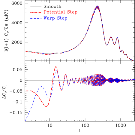
where the improvement is measured against the best fit smooth model. In contrast, the best fit model of Ref. Ade:2013rta had and a similar amplitude and frequency with a .111The original version of the Planck collaboration analysis Ade:2013rta [arXiv:1303.5082v1] erroneously conflated with (see Eq. 94) and correcting this definition also brings the amplitude into agreement with that found for WMAP Adshead:2011jq . As shown in Tab. 3, this difference is not due to the inclusion of second order corrections from in Eq. (5) though their omission would bias cosmological parameters such as and . The Planck data thus favor oscillations at the few percent level in , with a peak-to-peak spacing of . Note that at , the damping suppression and for this model corresponds to . Thus the oscillations persists at least out to the second acoustic peak (see Fig. 2).
The complete list of cosmological parameters for the best fit step model is listed in Tab.3. The oscillations add broadband power and generally require a lower normalization. Because in this model they damp near the well-constrained third peak, this also requires a higher tilt to keep the total power fixed at this best constrained region. As a result, the model has slightly smaller broadband power at low multipoles, reaching at the quadrupole.
Furthermore, the Planck data are also compatible with oscillations that persist out to the highest multipole measured in the data . Taking , which is indistinguishable from infinity for Planck,
| (15) |
This fit only differs in by 2.6 from that of the global minimum and is comparable to the best fit found in Ref. Ade:2013rta . Note that even with no damping scale in curvature fluctuations, oscillations in decline with due to projection and lensing effects (see Adshead:2011jq and Eq. 94). Had we fixed cosmological parameters to the best fit smooth model then this would be falsely penalized by . The cosmological parameters for this model are also given in Tab. 3. Notably with no damping scale, the tilt no longer requires significant adjustment. The change in mainly reflects slightly different cosmological parameters that produce correspondingly different distances to recombination rather than a change in the angular scale.
In summary, the Planck data favor percent level oscillations in produced by potential step features by with two parameters that control the oscillation frequency and amplitude. Minimizing the for damping of the oscillations confines the oscillations to roughly the first and second peaks and marginally improves the fit with an additional for a total of with one additional parameter for a total of three.
III.2 Low Sound Speed Models
Low sound speed DBI models allow for two different classes of steps with two different phenomenologies that impact low multipoles in the Planck data. Both steps in the potential and warp produce the same high multipole oscillations driven by the amplitude parameter . Given a that minimizes the Planck at high multipole, the remaining freedom is in choosing a sound speed after the step . In both the potential and warp scenarios, this uniquely fixes the two remaining step parameters and . Recall that controls the step in the power spectrum around the first oscillation and controls the shape of the first few oscillations. Since the fit is driven by the oscillations with only small impact from and , we fix all the other parameters to the global minimum of Eq. (III.1) when examining the impact of .
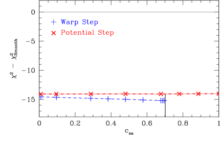
For potential steps, and . Even for the maximal case of and , there is very little impact on the CMB power spectrum. Consequently as shown in Fig. 3 the surface is essentially flat across .
For warp steps both and can be greater than unity and the sound speed has a larger fractional effect on . However, their impact is still limited to the first few oscillations and, given the preference for a horizon scale , severely cosmic variance limited. Raising mainly enhances the step in the power spectrum relative to the oscillations thus lowering the first few multipoles. Both and are important in establishing the shape due to a cancellation in their effects at the first oscillation.
Since warp steps do not produce oscillatory features as , there is a maximum for which they can explain the oscillations (see Fig. 3). The best fit has the maximal possible sound speed
| (16) |
which implies , given the fixed parameters in Eq. (III.1). While the step in the curvature power spectrum is approximately (see Fig. 9) in , this and the changes in the cosmological parameters translates into a suppression of power at the quadrupole relative to the smooth model (see Fig. 2). Note that the drop between is particularly sharp for warp steps due to a local maximum in the curvature spectrum oscillations. Nonetheless, with cosmic variance these changes have only a small impact on the fit. As a consequence, while warp steps have interesting phenomenology that may ameliorate low multipole anomalies, there is no statistically significant preference for .
IV Future Tests
While an improvement of for two parameters and up to in the full step parameter space may sound significant, it has been shown that for more flexible oscillatory models, where not only the amplitude and frequency but also the phase of the oscillation is fit, realizations of smooth models with noise often recover this level of improvement, albeit typically with a smaller oscillation amplitude Meerburg:2013cla . Furthermore the improvement in the WMAP likelihood Adshead:2011jq ; Meerburg:2013cla is comparable to that of the Planck likelihood despite the higher precision of Planck whereas one would have expected the latter to increase for a true signal. For these reasons, it is important to have more definitive tests for the origin of these improvements. In this section we discuss predictions of the best fit models identified above that may be used to verify or falsify the hypothesis of their primordial origin.
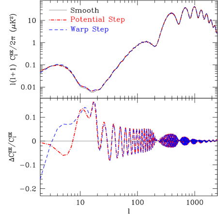
As emphasized by Ref. Mortonson2009 , the most incisive consistency test for inflationary features is the -mode polarization power spectrum and cross spectrum. In Fig. 4 (left panel), we show the predicted -mode power spectrum of the models in Fig. 2. Consistency with inflationary oscillations demands that oscillations appear at the same frequency while modulated by the acoustic transfer to have nodes that are out of phase with the temperature. Furthermore due to projection effects, the polarization oscillations are twice as prominent in polarization. In principle, the low polarization can also more than double the distinguishing power between the warp and potential fits, albeit limited in practice by galactic foregrounds and uncertainties in the reionization model.
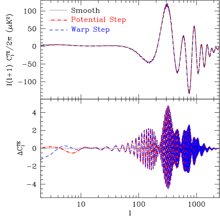
Finally, the temperature-polarization cross spectrum must also exhibit consistent oscillations as shown in Fig. 4 (right panel). These predictions should be tested in the next release of the Planck data. More generally they can be tested in any CMB polarization data set that has sufficient amounts of sky to distinguish modes separated by and oscillations in power of 3-10%.
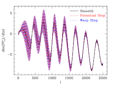
The best fit oscillatory models also predict different CMB lensing effects. High frequency features act in a similar fashion as the acoustic peaks in providing a signal for lensing. The fineness of the features compared with the acoustic spacing of offsets the smallness of the amplitude. In Fig. 5, we quantify this expectation by showing for the smooth and best fit step models
| (17) |
which controls lensing and squeezed bispectrum effects Lewis:2011fk . Note that what was a small effect for the power spectrum is an order unity effect for certain lensing effects.
There are two related ways in which the oscillations impact lensing observables. First, if lensing reconstruction were performed with the oscillatory models to construct the filters in the optimal quadratic estimator rather than the smooth models, the noise power in the reconstruction should decrease if the oscillatory features are real. To see this note that in the flat-sky approximation the sample-variance limited reconstruction noise power of the lensing potential is given by Hu:2001tn ; Lewis:2011fk
| (18) |
where . For , and for , can be Taylor expanded around . The numerator then scales as the derivative in Eq. (17) squared. For the best fit models, this changes the noise for .
Relatedly, lensing by long-wavelength modes modulates the angular scale of features in the power spectrum which itself is correlated with the CMB temperature anisotropy through the ISW effect. Thus the presence of fine scale oscillations changes the squeezed reduced bispectrum of temperature fluctuations Goldberg:1999xm
| (19) |
where is the correlation of the ISW temperature and lensing potential fields. The permutation of again makes the result scale as the derivative of and is enhanced by the oscillation. Both of these lensing effects are in principle detectable, though for the best fit frequency with the impact will be limited by cosmic variance. A more detailed study is required to determine their effects on the existing Planck data set.
Features during inflation also produce primordial non-Gaussianity in mainly the equilateral configuration Chen:2006xjb ; Adshead:2011bw ; Adshead:2012xz ; Achucarro:2012fd . For the best fit step models these should also be observable in Planck Adshead:2011jq ; Adshead:2013zfa . Extracting these signals though will require using specific templates that include these rapid oscillations Fergusson:2010dm . Since the equilateral bispectrum amplitude scales as , the lack of a strong bound on the damping scale implies that the bispectrum signal could be very large at high multipole, though these models would be beyond the regime of validity of the effective field theory that underlies their calculation Baumann:2011su
Thus if the oscillatory fits really reflect inflationary features, there is a battery of consistency tests that the CMB temperature and polarization anisotropy must satisfy.
V Discussion
In this paper, we have extended and improved the modeling and analysis of sharp inflationary steps for the Planck CMB power spectrum. We find that for the two parameters of the amplitude and frequency of the oscillations, step models improve the fit by whereas additional parameters such as the finite width of the step and sound speed of the inflaton marginally improve the fit to and respectively. In particular, sound speed effects for warp steps lower the quadrupole power by .
We have shown that it is critical to jointly fit step and cosmological parameters simultaneously. If cosmological parameters, especially the amplitude and tilt, are held fixed then one would falsely infer that the oscillations must damp away at high multipole due to their excess average power. We have shown that on the contrary there is only marginal preference for a finite damping scale. The improvement in modeling to second order terms in the generalized slow roll approximation developed here is also required by the increased precision of Planck at high multipoles but their omission would mainly bias the cosmological parameters rather than degrade the fit itself.
Given that chance features in the noise can masquerade as oscillatory step features Meerburg:2013cla , we have also provided a suite of consistency tests that can verify or falsify the primordial origin of these improved fits. The polarization power and cross spectra should reveal a matching and larger set of oscillations modulated by an out of phase acoustic transfer. The oscillations, if primordial, also provide an extra signal for CMB lensing reconstruction and squeezed bispectra from the lensing-ISW correlation. Finally, the primordial non-Gaussianity in equilateral bispectrum configurations should also be observable. These predictions may soon be tested in the next release of Planck data.
Acknowledgements.
We thank Peter Adshead, Aurelien Benoit-Levy, Douglas H. Rudd and Shi Chun Su for useful discussions. WH was supported by the Kavli Institute for Cosmological Physics at the University of Chicago through grants NSF PHY-0114422 and NSF PHY-0551142 and an endowment from the Kavli Foundation and its founder Fred Kavli. VM and WH were additionally supported by U.S. Dept. of Energy contract DE-FG02-90ER-40560, WH by the David and Lucile Packard Foundation and VM by the Brazilian Research Agency CAPES Foundation and by U.S. Fulbright Organization.Appendix A Analytic Step Spectrum
In this Appendix, we derive and test the analytic model for the power spectrum used in the main paper, extending previous treatments Adshead:2011jq ; Miranda:2012rm for large, sharp steps in the warp and potential in the DBI context. These necessitate second order corrections to achieve the precision required for the Planck data. We begin with a brief review of the generalized slow roll (GSR) approximation Stewart:2001cd ; Hu:2011vr for large power spectrum features in §A.1 Dvorkin:2009ne . In §A.2, we use exact energy conservation and the attractor solutions before and after the step to derive the general analytic model for the power spectrum in the GSR approximation. In §A.3, A.4 we apply this model to steps in the warp and potential.
A.1 Generalized Slow Roll
In a general model for inflation, the comoving curvature power spectrum,
| (20) |
is evaluated by solving the field or modefunction equation in spatially flat gauge Garriga:1999vw ; Hu:2011vr
| (21) |
Here deviations from de Sitter space are characterized by
| (22) |
where
| (23) |
with as efolds with as the end of inflation, denotes the sound speed of field fluctuations, and
| (24) |
denotes the sound horizon. Here and throughout .
Eq. (21) can be formally solved with the Green function technique by taking its right hand side as an external source given by the de Sitter mode function with Bunch-Davies initial conditions
| (25) |
and iteratively improving the solution for the presence of the deviations introduced by . Including the leading second order correction for large features, the power spectrum is given by Choe:2004zg ; Dvorkin:2009ne
| (26) | ||||
where the source function
| (27) |
and recall is given by Eq. (II). The validity of the approximation relies on the deviations in the modefunctions or the curvature being small rather than the deviations from slow roll. It is monitored by the second order corrections
| (28) |
with and given by Eq. (II). The GSR approximation itself will begin to break down unless Dvorkin:2011ui
| (29) |
.
Finally, carries both the smooth tilt type deviations from scale invariance as well as any impact of sharp features. For sharp features it can be approximated by Miranda:2012rm
| (30) |
where the additional slow-roll parameters are defined by
| (31) |
and we reabsorb the slow roll deviations in these parameters into the factor. Thus modeling a sharp feature amounts to determining its impact on and .
A.2 Step Sources
We consider sharp steps in the warp and potential of the DBI Lagrangian (1) which generate analogous changes in and . To keep our treatment general, we first parameterize the evolution of these quantities relying on energy conservation and the attractor solution to define their functional form. In the following subsections we give the correspondence of this parameterization to specific step parameters.
The energy density of the inflaton
| (32) |
is conserved as long as the inflaton rolls across the step in much less than an efold. This conservation then gives the relationship between the sound speed before (“”; ) and immediately after (“”; ) the step. The acceleration equation
| (33) |
then gives the corresponding change in . After the step, the rolling of the inflaton
| (34) |
differs from the friction dominated attractor solution
| (35) |
to which it must decay on the expansion time scale or well after the inflaton has crossed the step (“”). These relations hold for arbitrarily large steps so long as .
Together, they imply that the functional form of and is generically given by Miranda:2012rm
| (36) | ||||
where for convenience we have scaled the quantities to their values on the attractor after the step
| (37) |
Here represents a step of infinitesimal width at normalized to before the step and after. We discuss the impact of the finite width below.
Following Ref. Miranda:2012rm , it is straightforward to derive the source function in the approximation that changes to and are small by taking their derivatives and integrals to form the quantities in Eq. (30). Note that this limit does not necessarily require the steps in the warp itself to be small. In the limit of a large warp factor , the sound speed approaches unity regardless of the form of and hence the change in the sound speed are small even for a large fractional change in .
Integrals over are then simply evaluated by recalling that is a delta function of amplitude 2. The result of integrating the source by parts is
| (38) |
where
| (39) |
for the leading order GSR contribution in Eq. (26) which, once corrected for the finite width of the step below, we shall call GSR0. Here we have replaced the parameter in Eq. (26) with the power spectrum normalization at . Note that
| (40) |
which is given in closed form in Eq. (II).
Given that
| (41) |
we can further interpret the meaning of the coefficients. represents a step in the power spectrum and its amplitude is determined by the fact that the inflaton is on the attractor solution before and well after the step. provides a constant amplitude oscillation whose value is determined by the sharpest part of the feature: the fractional changes in and right at the step. Finally modifies the shape of the first few oscillations due to the source.
Likewise the first order corrections are given by
| (42) |
where
| (43) |
which is given in closed form in Eq. (II).
We call the analytic model with the correction GSR1. Using Eq. (29), we thus expect the GSR expansion itself to be under control for so long as
| (44) |
At , the exact requirement is a model dependent restriction on a combination of , , but in the warp and potential step examples this gives roughly the same criteria for the step height.
In principle this domain of validity includes fractional deviations in and that approach unity, including the region of interest for Planck. However although the GSR expansion itself remains under control, Eq. (39) is derived by assuming small fractional deviations and requires correction. Just as we extended the validity of the step approximation to nonlinearities in the step amplitude above, we can also approximately correct for weak nonlinearity in the slow roll parameters by rescaling the coefficients. Here we extend and generalize the approach of Ref. Adshead:2011jq and Miranda:2012rm for arbitrary sound speeds.
The amplitude gives the step in power and hence the slow roll attractor determines it as
| (45) |
The changes in and at the step are already determined nonlinearly and so the only further correction to comes from the conversion to slow-roll parameters, e.g. . Following Ref. Adshead:2011jq , we evaluate and at the midpoint of the step and hence
| (46) |
Finally for , while there is no direct nonlinear constraint to determine its amplitude, by also renormalizing to the midpoint of the step we approximately preserve the relative relationship between the coefficients that determines the shape of their combined contributions. This is especially important for warp steps where cancellations between and occur around the first oscillation. Thus, we take
| (47) |
Finally, we can account for the finite width of the step. If we replace the step function with a function
| (48) |
the integrals over will not contribute if the windows in Eq. (II) oscillate many times over the width of the step . This causes a damping such that the coefficients in Eqs. (A.2) and (42) are replaced by Adshead:2011jq
| (49) |
where the damping function
| (50) |
with the damping scale
| (51) |
The derivation of Eq. (5) for the functional form for the analytic model of the step power spectrum is thus complete. We now turn to specific forms for warp and potential steps.
A.3 Warp Steps
For steps in the warp , we have before and after the step
| (52) |
and we can then use energy conservation and the attractor solution to give the relevant and parameters of the model in Eq. (37). Our convention is to quote these in terms of and the sound speed on the attractor after the step . The attractor solution tells us that
| (53) |
and using Eq. (33) for , we obtain
| (54) |
Now let us consider the sharp changes immediately after the step. Energy conservation tells us
| (55) |
or
| (56) |
and with Eq. (33)
| (57) |
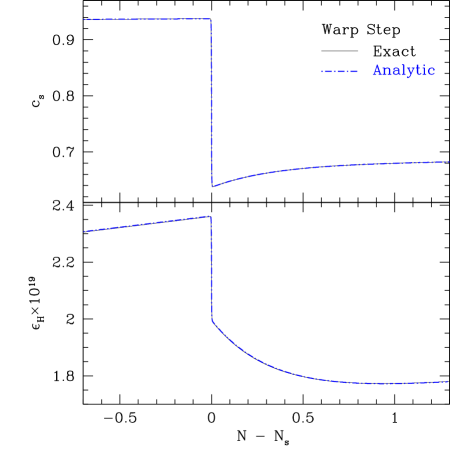
We show an example of the evolution of and in Fig. 6. Since the analytic model only captures the evolution of the parameters around the step and not the evolution on the slow roll attractor, we plot
| (58) |
where is the analytic model of Eq. (36), is the attractor on either side of the step and is evaluated approaching the step from either side with approached from the side after the step. We likewise account for the slow roll evolution of . In practice, rather than iterating the attractor solution of Eq. (35) in the equations of motion to the required accuracy we numerically solve the equivalent smooth model before and after the step to determine .
We can now use the general description of Eqs. (45), (46), (47) to give the coefficients of the analytic power spectrum form. Note that in the small step limit,
| (59) |
and so
| (60) |
in agreement with Ref. Miranda:2012rm . Our generalized expression lets us explore the limit
| (61) |
Note that for finite these limits are all finite and so the maximal amplitudes are also bounded
| (62) |
Thus for a fixed observed oscillation amplitude there is always a maximum for which a warp step cannot explain the data
| (63) |
For example, if , .

A.4 Potential Steps
For potential steps
| (64) |
The attractor solution says that to leading order in , there is no net change in or only a transient deviation at the step. Thus and () or
| (65) |
We can also use the attractor to eliminate using
| (66) |
Energy conservation then gives the transient change as
| (67) |
and using Eq. (33)
| (68) |
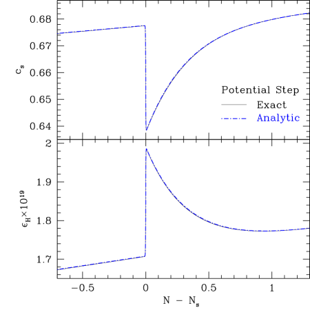
The general description of Eqs. (45), (46), (47) then gives the coefficients of the analytic power spectrum form. We show an example of the evolution of and in Fig. 8. Again, to capture the slow roll evolution of the smooth model, we plot the analytic model corrected as in Eq. (58).
In the limit of a small potential step
| (69) |
and so
| (70) |
which generalizes the results of Ref. Adshead:2011jq to arbitrary sound speed. The sound speed experiences a transient dip for downward steps .
Note that in the opposite limit
| (71) |
and so
| (72) |
Since these amplitudes are beyond the limits of the GSR approximation itself according to Eq. (44), there is effectively no relevant bound on the oscillation amplitude set by energy conservation and the attractor solution unlike the warp step case. Likewise, for a given , there is no bound on the required sound speed.
Appendix B Power Spectrum Accuracy
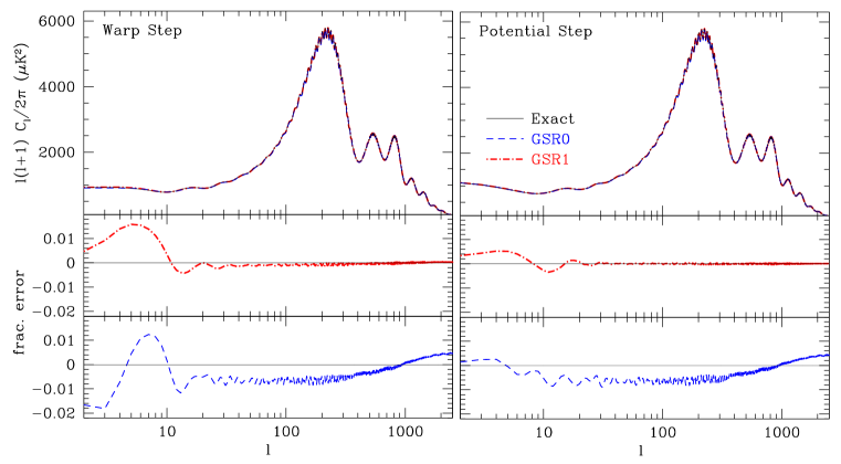
In this section, we test the accuracy of the leading order GSR0 approximation used in previous analyses Adshead:2011jq and the first order GSR1 corrections discussed in Appendix A against an exact computation of the power spectrum from the DBI Lagrangian of Eq. (1). Although GSR0 was previously demonstrated to be sufficiently accurate for WMAP data Adshead:2011jq ; Miranda:2012rm , we show here that the increase in precision to the level in Planck requires second order corrections.
The exact computation of the power spectrum follows from solving Eq. (21) for a DBI step model that is parameterized by , defining the broadband amplitude and slope of the power spectrum, and the step parameters defining the step position, height parameters, and width (see Miranda:2012rm for computational details). For testing purposes, we choose
| (73) |
and
| (74) |
For the warp step, we choose
| (75) |
and for the potential step
| (76) |
These parameters are in fact chosen to be close to the Planck maximum likelihood solution for the amplitude and frequency of warp step oscillations by inverting the steps in this test. Notice that in that case, the fractional change in the warp exceeds unity. The width is set so that damping occurs in the region that Planck is most sensitive to so as to yield the most stringent test of accuracy. The cosmological parameters for the test are given in Tab. 1 and coincide with the best fit model without a step.
The analytic models are specified by the conversion of the fundamental parameters into the amplitude parameters , the sound horizon at the step , the effective number of oscillations before damping , as well as the broadband amplitude and tilt parameters and .
Given a solution to the background equations without the step, we set the parameters
| (77) |
according to their values at . The amplitude parameters are then determined by Eqs. (45-(47) such that
| (78) |
and
| (79) |
Next, the physical scale associated with the step has to be set very precisely in order not to have a phase error after many oscillations. We follow Ref. Miranda:2012rm in defining it numerically to be the sound horizon at which the deviation in the GSR source function due to the step is appropriately centered to a small fraction of the step width
| (80) |
Using this definition we obtain
| (81) |
Note that although the step is at the same position in field space in both cases, the sound horizon differs slightly due to the change in .
For the damping parameter, we likewise convert the field width to a physical width with the numerical solution for through
| (82) |
For the test cases, we obtain
Finally there are the broadband power parameters and . For the tilt parameter, which is slowly varying and essentially independent of the step, we take the slope at Mpc-1 of the model with . We have chosen parameters in Eq. (73) so that coincides with the value given in Tab. 1. On the other hand, the effective amplitude depends on the presence of the step as well as the order of the GSR approximation used. In Eq. (A.2), the broadband power gains a contribution from the average of the oscillations
where here is the modified Bessel function, not to be confused with the GSR integral . This non-zero average is the fundamental reason why cosmological parameters must be varied jointly with the step parameters when analyzing the Planck data. In the first order correction Eq. (26), there is the analogous averaging effect
| (84) |
which is also despite being higher order in the GSR approximation. Moreover, around the damping scale set by the broadband average of the oscillation changes with in Eq. (B)-(84) and is not purely an amplitude shift. Note that the error induced by this average term scales as and so rapidly increases with the amplitude of the oscillations.
Since the best choice for depends on both the method and the data set considered, we choose as the amplitude which gives the best agreement between the exact computation and the given GSR computation for the Planck dataset. We therefore use the Planck likelihood itself to define for each method. In order to remove the ambiguity caused by the exact model not possessing the maximum likelihood normalization, we in practice maximize both the Planck likelihood over to obtain and a rescaling of the amplitude of the exact model by to obtain its best normalization. We then set to remove the rescaling.
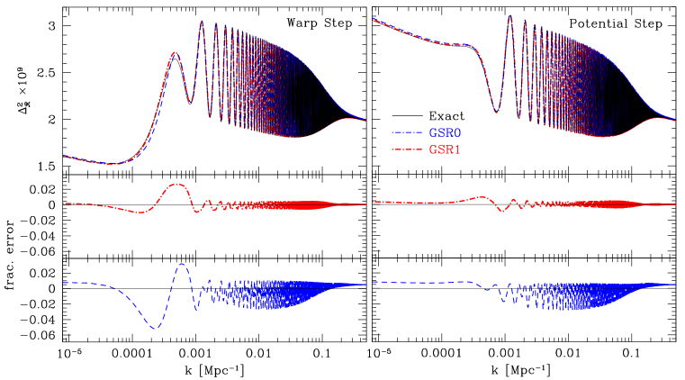
In Fig. 10 we show the residual errors in the GSR0 and GSR1 after the normalization has been set in this way. Note that the residuals cross zero at , reflecting the pivot or best constrained portion of the Planck spectrum. For scales much smaller than or much larger than the damping scale of the oscillation, the difference between GSR0, GSR1, and exact is nearly constant and can be absorbed into the normalization. However in our test case, which we have chosen to be the worst case scenario, the damping falls exactly at the pivot. The result is that even with the best fit normalization, GSR0 produces errors that pivot around . While the error in GSR0 can mainly be absorbed by adjusting cosmological parameters such as the tilt, they are large enough to bias such parameters non-negligibly. These residuals are reduced to the level with the GSR1 approximation.
More quantitatively, for these specific test cases the residuals produce a change in the Planck likelihood versus exact of
| (85) |
and
| (86) |
Thus the GSR1 approximation is sufficiently accurate for the Planck analysis. In fact, the errors would be even smaller at its global minimum.
The error in these approximations also depends on the step parameter model. For reference if the error in the GSR0 approximation becomes for the warp step and for the potential step. Here the error is significantly lower since it takes the form of a constant amplitude rescaling which can be absorbed into .
In our examples the result of the normalization procedure is to set,
| (87) |
for the warp step and
| (88) |
for the potential step. In the absence of a step (), the same procedure would yield which is different from the GSR1 value. These changes reflect the broadband power introduced by the oscillations in each case. Given the precision of the Planck data these differences are significant and cannot be held fixed when fitting to step models.
For the minimization procedure in Appendix C, it is nonetheless useful to have an approximate prescription for the renormalization of in the presence of oscillations. Given the average of the oscillatory pieces in Eq. (B-84), the normalization parameter that the data should hold approximately fixed is
| (89) |
where contains the average of the oscillatory pieces in each approximation
| (90) |
Here the factor accounts for the change in the heights of the acoustic peaks due to anisotropy suppression by scattering during reionization. In our test cases
| (91) |
for the warp step,
| (92) |
for the potential step and without a step. Note that absorbs most of the changes in the normalization given in Eq. (87-88) from the presence of the step.
Appendix C Minimization
In this Appendix we provide details of the effective minimization for the various models presented in §III. In each case, we use the MIGRAD variable metric minimizer from the CERN Minuit2 code James:1975dr .
We begin with the smooth CDM cosmology specified by the cosmological parameters , and 14 foregrounds parameters defined in the Planck likelihood Planck:2013kta . We include the Planck low- spectrum (Commander, ), the high- spectrum (CAMspec, ) and WMAP9 polarization (lowlike) likelihoods in our analysis Planck:2013kta ; Bennett:2012fp . is the effective normalization defined in Eq. (89); in the absence of a step . In the standard CDM model, the effective number and sum of the masses of neutrinos are held fixed to and respectively with the helium fraction . The best fit model is given in Tab. 1 and 2 and its is the baseline from which we quantify any improvements due to the step parameters. We fix the foreground parameters to these values for the following analysis but have spot checked that reoptimization over the foreground parameters does not substantially change our results.
| GSR1 | GSR0 | |||
For the step analysis, the starting point is the canonical potential step where . As the oscillatory features from dominate the fit to the Planck data, the other cases are built from this model. In this case the step is described by . While we could directly minimize the in this joint cosmological and step parameter space, the efficiency of the search is greatly improved by choosing parameters that are better aligned to the principle axes of the surface.
The angular frequency of the oscillation changes with cosmological parameters at fixed . It is thus advantageous to replace with
| (93) |
where is the distance to recombination. Note that the oscillations in are then described by sinusoids such as . Next, due to projection effects, a fixed amplitude produces an oscillation in that decays as . In Ref. Adshead:2011jq this scaling was approximately accounted for in the curvature power spectrum description by introducing the amplitude parameter
| (94) |
we adopt this convention rather than the more orthogonal angular approach in order to compare with the previous literature. Note that the original version of the Planck collaboration analysis erroneously conflated this parameter with Ade:2013rta .
Finally, given that the oscillations produce excess broadband power, we use the normalization parameter as defined in Eq. (89). For the best fit models, this parameter rather than itself is nearly constant. The optimized parameters are therefore for the smooth cosmology and for the step. The minimum potential step model with is given in Tab. 3 (GSR1 column) and represents an improvement of over the smooth model of Tab. 1. For reference we also show here the best fit model at , where the oscillations are undamped all the way to the maximum of for Planck. Note that most of the improvement due to the step remains. We also repeat the minimization for the GSR0 approximation used in previous treatments for comparison. Note that after adjusting cosmological parameters, steps in either approximation fit equally well but the recovery of such parameters would be biased by using the less accurate GSR0 approximation.
For the arbitrary sound speed warp and potential step models, and are set consistently with the step amplitude and slow roll parameters after the step through Eq. (II). These parameters mainly change the power spectrum around and hence produce only small changes in the due to the limitations of cosmic variance.
We therefore keep the other parameters fixed to the values of model listed in Tab. 3 when considering the additional freedom in these models. Given a fixed , which fixes the amplitude of the step, this freedom is parameterized by , the sound speed after the step. For warp step, the best fit is given by
| (95) |
and this corresponds to a improvement over the potential step model at . For low sound speed potential step models, the limit provides the best fit
| (96) |
Given the additional parameter , neither improvement is statistically significant.
References
- (1) R. Flauger, L. McAllister, E. Pajer, A. Westphal, and G. Xu, JCAP 1006, 009 (2010), arXiv:0907.2916 [hep-th]
- (2) P. Adshead, C. Dvorkin, W. Hu, and E. A. Lim, Phys.Rev. D85, 023531 (2012), arXiv:1110.3050 [astro-ph.CO]
- (3) H. Peiris, R. Easther, and R. Flauger, JCAP 1309, 018 (2013), arXiv:1303.2616 [astro-ph.CO]
- (4) P. D. Meerburg, D. N. Spergel, and B. D. Wandelt(2013), arXiv:1308.3704 [astro-ph.CO]
- (5) P. Ade et al. (Planck Collaboration)(2013), arXiv:1303.5082 [astro-ph.CO]
- (6) R. Easther and R. Flauger(2013), arXiv:1308.3736 [astro-ph.CO]
- (7) M. Benetti(2013), arXiv:1308.6406 [astro-ph.CO]
- (8) P. D. Meerburg and D. N. Spergel(2013), arXiv:1308.3705 [astro-ph.CO]
- (9) X. Chen, R. Easther, and E. A. Lim, JCAP 0706, 023 (2007), arXiv:astro-ph/0611645 [astro-ph]
- (10) E. Silverstein and D. Tong, Phys.Rev. D70, 103505 (2004), arXiv:hep-th/0310221 [hep-th]
- (11) J. A. Adams, B. Cresswell, and R. Easther, Phys. Rev. D64, 123514 (2001), arXiv:astro-ph/0102236
- (12) R. Bean, X. Chen, G. Hailu, S.-H. Tye, and J. Xu, JCAP 0803, 026 (2008), arXiv:0802.0491 [hep-th]
- (13) V. Miranda, W. Hu, and P. Adshead, Phys.Rev. D86, 063529 (2012), arXiv:1207.2186 [astro-ph.CO]
- (14) C. Dvorkin and W. Hu, Phys.Rev. D82, 043513 (2010), arXiv:1007.0215 [astro-ph.CO]
- (15) A. Lewis, A. Challinor, and A. Lasenby, Astrophys. J. 538, 473 (2000), astro-ph/9911177
- (16) C. Howlett, A. Lewis, A. Hall, and A. Challinor, JCAP 1204, 027 (2012), arXiv:1201.3654 [astro-ph.CO]
- (17) M. J. Mortonson, C. Dvorkin, H. V. Peiris, and W. Hu, Phys. Rev. D79, 103519 (2009), arXiv:0903.4920 [astro-ph.CO]
- (18) A. Lewis, A. Challinor, and D. Hanson, JCAP 1103, 018 (2011), arXiv:1101.2234 [astro-ph.CO]
- (19) W. Hu, Astrophys.J. 557, L79 (2001), arXiv:astro-ph/0105424 [astro-ph]
- (20) D. M. Goldberg and D. N. Spergel, Phys.Rev. D59, 103002 (1999), arXiv:astro-ph/9811251 [astro-ph]
- (21) P. Adshead, W. Hu, C. Dvorkin, and H. V. Peiris, Phys.Rev. D84, 043519 (2011), arXiv:1102.3435 [astro-ph.CO]
- (22) P. Adshead and W. Hu, Phys.Rev. D85, 103531 (2012), arXiv:1203.0012 [astro-ph.CO]
- (23) A. Achucarro, J.-O. Gong, G. A. Palma, and S. P. Patil, Phys.Rev. D87, 121301 (2013), arXiv:1211.5619 [astro-ph.CO]
- (24) P. Adshead, W. Hu, and V. Miranda, Phys.Rev. D88, 023507 (2013), arXiv:1303.7004 [astro-ph.CO]
- (25) J. Fergusson, M. Liguori, and E. Shellard, JCAP 1212, 032 (2012), arXiv:1006.1642 [astro-ph.CO]
- (26) D. Baumann and D. Green, JCAP 1109, 014 (2011), arXiv:1102.5343 [hep-th]
- (27) E. D. Stewart, Phys.Rev. D65, 103508 (2002), arXiv:astro-ph/0110322 [astro-ph]
- (28) W. Hu, Phys.Rev. D84, 027303 (2011), arXiv:1104.4500 [astro-ph.CO]
- (29) C. Dvorkin and W. Hu, Phys.Rev. D81, 023518 (2010), arXiv:0910.2237 [astro-ph.CO]
- (30) J. Garriga and V. F. Mukhanov, Phys.Lett. B458, 219 (1999), arXiv:hep-th/9904176 [hep-th]
- (31) J. Choe, J.-O. Gong, and E. D. Stewart, JCAP 0407, 012 (2004), arXiv:hep-ph/0405155 [hep-ph]
- (32) C. Dvorkin and W. Hu, Phys.Rev. D84, 063515 (2011), arXiv:1106.4016 [astro-ph.CO]
- (33) F. James and M. Roos, Comput.Phys.Commun. 10, 343 (1975)
- (34) P. Ade et al. (Planck collaboration)(2013), arXiv:1303.5075 [astro-ph.CO]
- (35) C. Bennett, D. Larson, J. Weiland, N. Jarosik, G. Hinshaw, et al.(2012), arXiv:1212.5225 [astro-ph.CO]