Hamiltonian Monte Carlo for Hierarchical Models

Abstract

Hierarchical modeling provides a framework for modeling the complex interactions typical of problems in applied statistics. By capturing these relationships, however, hierarchical models also introduce distinctive pathologies that quickly limit the efficiency of most common methods of inference. In this paper we explore the use of Hamiltonian Monte Carlo for hierarchical models and demonstrate how the algorithm can overcome those pathologies in practical applications.

Many of the most exciting problems in applied statistics involve intricate, typically high-dimensional, models and, at least relative to the model complexity, sparse data. With the data alone unable to identify the model, valid inference in these circumstances requires significant prior information. Such information, however, is not limited to the choice of an explicit prior distribution: it can be encoded in the construction of the model itself.

Hierarchical models take this latter approach, associating parameters into exchangeable groups that draw common prior information from shared parent groups. The interactions between the levels in the hierarchy allow the groups to learn from each other without having to sacrifice their unique context, partially pooling the data together to improve inferences. Unfortunately, the same structure that admits powerful modeling also induces formidable pathologies that limit the performance of those inferences.

After reviewing hierarchical models and their pathologies, we’ll discuss common implementations and show how those pathologies either make the algorithms impractical or limit their effectiveness to an unpleasantly small space of models. We then introduce Hamiltonian Monte Carlo and show how the novel properties of the algorithm can yield much higher performance for general hierarchical models. Finally we conclude with examples which emulate the kind of models ubiquitous in contemporary applications.

I Hierarchical Models

Hierarchical models GelmanEtAl:2013 are defined by the organization of a model’s parameters into exchangeable groups, and the resulting conditional independencies between those groups. A one-level hierarchy with parameters $\left(\theta,\phi\right)$ and data $\mathcal{D}$, for example, factors as (Figure 1)

$$\pi\!\left(\theta,\phi|\mathcal{D}\right)\propto\prod_{i=1}^{n}\pi\!\left(\mathcal{D}_{i}|\theta_{i}\right)\pi\!\left(\theta_{i}|\phi\right)\pi\!\left(\phi\right).$$ (1)

A common example is the one-way normal model,

$$y_{i} \sim\mathcal{N}\!\left(\theta_{i},\sigma_{i}^{2}\right)$$

$$\theta_{i} \sim\mathcal{N}\!\left(\mu,\tau^{2}\right),\mbox{ for }i=1,\dots,I,$$ (2)

or, in terms of the general notation of (1), $\mathcal{D}=(y_{i},\sigma_{i})$, $\phi=(\mu,\tau)$, and $\theta=(\theta_{i})$. To ease exposition we refer to any elements of $\phi$ as global parameters, and any elements of $\theta$ as local parameters, even though such a dichotomy quickly falls apart when considering models with multiple layers.

Figure 1: In hierarchical models “local” parameters, $\theta$, interact via a common dependency on “global” parameters, $\phi$. The interactions allow the measured data, $\mathcal{D}$, to inform all of the $\theta$ instead of just their immediate parent. More general constructions repeat this structure, either over different sets of parameters or additional layers of hierarchy.

Unfortunately for practitioners, but perhaps fortunately for pedagogy, the one-level model (1) exhibits all of the pathologies typical of hierarchical models. Because the $n$ contributions at the bottom of the hierarchy all depend on the global parameters, a small change in $\phi$ induces large changes in the density. Consequently, when the data are sparse the density of these models looks like a “funnel”, with a region of high density but low volume below a region of low density and high volume. The probability mass of the two regions, however, is comparable and any successful sampling algorithm must be able to manage the dramatic variations in curvature in order to fully explore the posterior.

For visual illustration, consider the funnel distribution Neal:2003 resulting from a one-way normal model with no data, latent mean $\mu$ set to zero, and a log-normal prior on the variance $\tau^{2}=e^{v}$,

$$\pi\!\left(\theta_{1},\ldots,\theta_{n},v\right)\propto\prod_{i=1}^{n}\mathcal{N}\!\left(x_{i}|0,(e^{-v/2})^{2}\right)\mathcal{N}\!\left(v|0,3^{2}\right).$$

The hierarchical structure induces large correlations between $v$ and each of the $\theta_{i}$, with the correlation strongly varying with position (Figure 2). Note that the position-dependence of the correlation ensures that no global correction, such as a rotation and rescaling of the parameters, will simplify the distribution to admit an easier implementation.

Figure 2: Typical of hierarchical models, the curvature of the funnel distribution varies strongly with the parameters, taxing most algorithms and limiting their ultimate performance. Here the curvature is represented visually by the eigenvectors of $\sqrt{\left|\partial^{2}\log p\!\left(\theta_{1},\ldots,\theta_{n},v\right)/\partial\theta_{i}\partial\theta_{j}\right|}$ scaled by their respective eigenvalues, which encode the direction and magnitudes of the local deviation from isotropy.

II Common Implementations of Hierarchical Models

Given the utility of hierarchical models, a variety of implementations have been developed with varying degrees of success. Deterministic algorithms, for example PinheiroEtAl:2000 ; RabeEtAl:2008 ; RueEtAl:2009 , can be quite powerful in a limited scope of models. Here we instead focus on the stochastic Markov Chain Monte Carlo algorithms, in particular Metropolis and Gibbs samplers, which offer more breadth.

II.1 Naïve Implementations

Although they are straightforward to implement for many hierarchical models, the performance of algorithms like Random Walk Metropolis and the Gibbs sampler RobertEtAl:1999 is limited by their incoherent exploration. More technically, these algorithms explore via transitions tuned to the conditional variances of the target distribution. When the target is highly correlated, however, the conditional variances are much smaller than the marginal variances and many transitions are required to explore the entire distribution. Consequently, the samplers devolve into random walks which explore the target distribution extremely slowly.

As we saw above, hierarchical models are highly correlated by construction. As more groups and more levels are added to the hierarchy, the correlations worsen and naïve MCMC implementations quickly become impractical (Figure 3).

Figure 3: One of the biggest challenges with modern models is not global correlations but rather local correlations that are resistant to the corrections based on the global covariance. The funnel distribution, here with $N=100$, features strongly varying local correlations but enough symmetry that these correlations cancel globally, so no single correction can compensate for the ineffective exploration of (a) the Gibbs sampler and (b) Random Walk Metropolis. After 2500 iterations neither chain has explored the marginal distribution of $v$, $\pi\!\left(v\right)=\mathcal{N}\!\left(v|0,3^{2}\right)$. Note that the Gibbs sampler utilizes a Metropolis-within-Gibbs scheme as the conditional $\pi\!\big{(}v|\vec{\theta}\big{)}$ does not have a closed-form.

II.2 Efficient Implementations

A common means of improving Random Walk Metropolis and the Gibbs sampler is to correct for global correlations, bringing the conditional variances closer to the marginal variances and reducing the undesired random walk behavior. The correlations in hierarchical models, however, are not global but rather local and efficient implementations require more sophistication. To reduce the correlations between successive layers and improve performance we have to take advantage of the hierarchical structure explicitly. Note that, because this structure is defined in terms of conditional independencies, these strategies tend to be more natural, not to mention more successful, for Gibbs samplers.

One approach is to separate each layer with auxiliary variables LiuEtAl:1998 ; LiuEtAl:1999 ; GelmanEtAl:2008 , for example the one-way normal model (2) would become

$$\theta_{i}=\mu+\xi\eta_{i},\ \eta_{i}\sim\mathcal{N}\!\left(0,\sigma^{2}_{\eta}\right),$$

with $\tau=|\xi|\sigma_{\eta}$. Conditioned on $\eta$, the layers become independent and the Gibbs sampler can efficiently explore the target distribution. On the other hand, the multiplicative dependence of the auxiliary variable actually introduces strong correlations into the joint distribution that diminishes the performance of Random Walk Metropolis.

In addition to adding new parameters, the dependence between layers can also be broken by reparameterizing existing parameters. Non-centered parameterizations, for example PapaspiliopoulosEtAl:2007 , factor certain dependencies into deterministic transformations between the layers, leaving the actively sampled variables uncorrelated (Figure 4). In the one-way normal model (2) we would apply both location and scale reparameterizations yielding

$$y_{i} \sim\mathcal{N}\!\left(\vartheta_{i}\tau+\mu,\sigma_{i}^{2}\right)$$

$$\vartheta_{i} \sim\mathcal{N}\!\left(0,1\right),$$

effectively shifting the correlations from the latent parameters to the data. Provided that the the data are not particularly constraining, i.e. the $\sigma_{i}^{2}$ are large, the resulting joint distribution is almost isotropic and the performance of both Random Walk Metropolis and the Gibbs sampler improves.

Figure 4: In one-level hierarchical models with global parameters, $\phi$, local parameters, $\theta$, and measured data $y$, correlations between parameters can be mediated by different parameterizations of the model. Non-centered parameterizations exchange a direct dependence between $\phi$ and $\theta$ for a dependence between $\phi$ and $y$; the reparameterized $\vartheta$ and $\phi$ become independent conditioned on the data. When the data are weak these non-centered parameterizations yield simpler posterior geometries.

Unfortunately, the ultimate utility of these efficient implementations is limited to the relatively small class of models where analytic results can be applied. Parameter expansion, for example, requires that the expanded conditional distributions can be found in closed form (although, to be fair, that is also a requirement for any Gibbs sampler in the first place) while non-centered parameterizations are applicable mostly to models where the dependence between layers is given by a generalized linear model. To enable efficient inference without constraining the model we need to consider more sophisticated Markov Chain Monte Carlo techniques.

III Hamiltonian Monte Carlo for Hierarchical Models

Hamiltonian Monte Carlo DuaneEtAl:1987 ; Neal:2011 ; BetancourtEtAl:2011 utilizes techniques from differential geometry to generate transitions spanning the full marginal variance, eliminating the random walk behavior endemic to Random Walk Metropolis and the Gibbs samplers.

The algorithm introduces auxiliary momentum variables, $p$, to the parameters of the target distribution, $q$, with the joint density

$$\pi\!\left(p,q\right)=\pi\!\left(p|q\right)\pi\!\left(q\right).$$

After specifying the conditional density of the momenta, the joint density defines a Hamiltonian,

$$H\!\left(p,q\right) =-\log\pi\!\left(p,q\right)$$

$$=-\log\pi\!\left(p|q\right)-\log\pi\!\left(q\right)$$

$$=T\!\left(p|q\right)+V\!\left(q\right),$$

with the kinetic energy,

$$T\!\left(p|q\right)\equiv-\log\pi\!\left(p|q\right),$$

and the potential energy,

$$V\!\left(q\right)\equiv-\log\pi\!\left(q\right).$$

This Hamiltonian function generates a transition by first sampling the auxiliary momenta,

$$p\sim\pi\!\left(p|q\right),$$

and then evolving the joint system via Hamilton’s equations,

$$\frac{dq}{dt} =+\frac{\partial H}{\partial p}=+\frac{\partial T}{\partial p}$$

$$\frac{dp}{dt} =-\frac{\partial H}{\partial q}=-\frac{\partial T}{\partial q}-\frac{\partial V}{\partial q}.$$

The gradients guide the transitions through regions of high probability and admit the efficient exploration of the entire target distribution. For how long to evolve the system depends on the shape of the target distribution, and the optimal value may vary with position Betancourt:2013b . Dynamically determining the optimal integration time is highly non-trivial as naïve implementations break the detailed balance of the transitions; the No-U-Turn sampler preserves detailed balance by integrating not just forward in time but also backwards HoffmanEtAl:2011 .

Because the trajectories are able to span the entire marginal variances, the efficient exploration of Hamiltonian Monte Carlo transitions persists as the target distribution becomes correlated, and even if those correlations are largely local, as is typical of hierarchical models. As we will see, however, depending on the choice of the momenta distribution, $\pi\!\left(p|q\right)$, hierarchical models can pose their own challenges for Hamiltonian Monte Carlo.

Figure 5: Careful consideration of any adaptation procedure is crucial for valid inference in hierarchical models. As the step size of the numerical integrator is decreased (a) the average acceptance probability increases from the canonically optimal value of 0.651 but (b) the sampler output converges to a consistent distribution. Indeed, (c) at the canonically optimal value of the average acceptance probability the integrator begins to diverge. Here consistency is measured with a modified potential scale reduction statistic GelmanEtAl:1992 ; StanMan:2013 for the latent parameter $v$ in a (50 + 1)-dimensional funnel.

III.1 Euclidean Hamiltonian Monte Carlo

The simplest choice of the momenta distribution, and the one almost exclusively seen in contemporary applications, is a Gaussian independent of $q$,

$$\pi\!\left(p|q\right)=\mathcal{N}\!\left(p|0,\Sigma\right),$$

resulting in a quadratic kinetic energy,

$$T\!\left(p,q\right)=\frac{1}{2}p^{T}\Sigma^{-1}p.$$

Because the subsequent Hamiltonian also generates dynamics on a Euclidean manifold, we refer to the resulting algorithm at Euclidean Hamiltonian Monte Carlo. Note that the metric, $\Sigma$, effectively induces a global rotation and rescaling of the target distribution, although it is often taken to be the identity in practice.

Despite its history of success in difficult applications, Euclidean Hamiltonian Monte Carlo does have two weaknesses that are accentuated in hierarchical models: the introduction of a characteristic length scale and limited variations in density.

III.1.1 Characteristic Length Scale

In practice Hamilton’s equations are sufficiently complex to render analytic solutions infeasible; instead the equations must be integrated numerically. Although symplectic integrators provide efficient and accurate numerical solutions HairerEtAl:2006 , they introduce a characteristic length scale via the time discretization, or step size, $\epsilon$.

Typically the step size is tuned to achieve an optimal acceptance probability BeskosEtAl:2013 , but such optimality criteria ignore the potential instability of the integrator. In order to prevent the numerical solution from diverging before it can explore the entire distribution, the step size must be tuned to match the curvature. Formally, a stable solution requires HairerEtAl:2006

$$\epsilon\sqrt{\lambda_{i}}<2$$

for each eigenvalue, $\lambda_{i}$, of the matrix

$$M_{ij}=\left(\Sigma^{-1}\right)_{ik}\frac{\partial^{2}V}{\partial q_{k}\partial q_{j}}.$$

Moreover, algorithms that adapt the step size to achieve an optimal acceptance probability require a relatively precise and accurate estimate of the global acceptance probability. When the chain has high autocorrelation or overlooks regions of high curvature because of a divergent integrator, however, such estimates are almost impossible to achieve. Consequently, adaptive algorithms can adapt too aggressively to the local neighborhood where the chain was seeded, potentially biasing resulting inferences.

Given the ubiquity of spatially-varying curvature, these pathologies are particularly common to hierarchical models. In order to use adaptive algorithms we recommend relaxing the adaptation criteria to ensure that the Markov chain hasn’t been biased by overly assertive adaptation. A particularly robust strategy is to compare inferences, especially for the latent parameters, as the adaptation criteria is gradually weakened, selecting a step size only once the inferences have stabilized and divergent transitions are rare (Figure 5). At the very least an auxiliary chain should always be run at a smaller step size to ensure consistent inferences.

III.1.2 Limited Density Variations

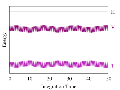
A more subtle, but no less insidious, vulnerability of Euclidean HMC concerns density variations with a transition. In the evolution of the system, the Hamiltonian function,

$$H\!\left(p,q\right)=T\!\left(p|q\right)+V\!\left(q\right),$$

is constant, meaning that any variation in the potential energy must be compensated for by an opposite variation in the kinetic energy. In Euclidean Hamiltonian Monte Carlo, however, the kinetic energy is a $\chi^{2}$ variate which, in expectation, varies by only half the dimensionality, $d$, of the target distribution. Consequently the Hamiltonian transitions are limited to

$$\Delta V=\Delta T\sim\frac{d}{2},$$

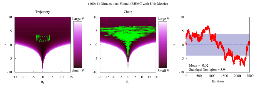
restraining the density variation within a single transition. Unfortunately the correlations inherent to hierarchical models also induce huge density variations, and for any but the smallest hierarchical model this restriction prevents the transitions from spanning the full marginal variation. Eventually random walk behavior creeps back in and the efficiency of the algorithm plummets (Figure 6, 7).

Figure 6: Because the Hamiltonian, $H$, is conserved during each trajectory, the variation in the potential energy, $V$, is limited to the variation in the kinetic energy, $T$, which itself is limited to only $d/2$.

Figure 7: Limited to moderate potential energy variations, the trajectories of Euclidean HMC, here with a unit metric $\Sigma=\mathbb{I}$, reduce to random walk behavior in hierarchical models. The resulting Markov chain explores more efficiently than Gibbs and Random Walk Metropolis (Figure 3), but not efficiently enough to make these models particularly practical.

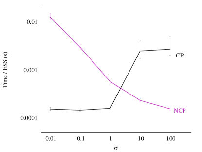
Because they remove explicit hierarchical correlations, non-centered parameterizations can also reduce the density variations of hierarchical models and drastically increase the performance of Euclidean Hamiltonian Monte Carlo (Figure 8). Note that as in the case of Random Walk Metropolis and Gibbs sampling, the efficacy of the parametrization depends on the relative strength of the data, although when the nominal centered parameterization is best there is often enough data that the partial pooling of hierarchical models isn’t needed in the first place.

Figure 8: Depending on the common variance, $\sigma^{2}$, from which the data were generated, the performance of a 10-dimensional one-way normal model (2) varies drastically between centered (CP) and non-centered (NCP) parameterizations of the latent parameters, $\theta_{i}$. As the variance increases and the data become effectively more sparse, the non-centered parameterization yields the most efficient inference and the disparity in performance increases with the dimensionality of the model. The bands denote the quartiles over an ensemble of 50 runs, with each run using Stan Stan:2013 configured with a diagonal metric and the No-U-Turn sampler. Both the metric and the step size were adapted during warmup, and care was taken to ensure consistent estimates (Figure 9).

Figure 9: As noted in Section III.1.1, care must be taken when using adaptive implementations of Euclidean Hamiltonian Monte Carlo with hierarchical models. For the results in Figure 8, the optimal average acceptance probability was relaxed until the estimates of $\tau$ stabilized, as measured by the potential scale reduction factor, and divergent transitions did not appear.

III.2 Riemannian Hamiltonian Monte Carlo

Euclidean Hamiltonian Monte Carlo is readily generalized by allowing the covariance to vary with position

$$\pi\!\left(p|q\right)=\mathcal{N}\!\left(p|0,\Sigma\!\left(q\right)\right),$$

giving,

$$T\!\left(p,q\right)=\frac{1}{2}p^{T}\Sigma^{-1}\left(q\right)p-\frac{1}{2}\log\left|\Sigma\!\left(q\right)\right|.$$

With the Hamiltonian now generating dynamics on a Riemannian manifold with metric $\Sigma$, we follow the convention established above and denote the resulting algorithm as Riemannian Hamiltonian Monte Carlo GirolamiEtAl:2011 .

The dynamic metric effectively induces local corrections to the target distribution, and if the metric is well chosen then those corrections can compensate for position-dependent correlations, not only reducing the computational burden of the Hamiltonian evolution but also relieving the sensitivity to the integrator step size.

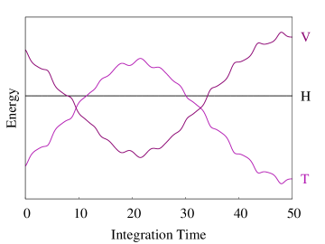
Note also the appearance of the log determinant term, $\frac{1}{2}\log\left|\Sigma\!\left(q\right)\right|$. Nominally in place to provide the appropriate normalization for the momenta distribution, this term provides a powerful feature to Riemannian Hamiltonian Monte Carlo, serving as a reservoir that absorbs and then releases energy along the evolution and potentially allowing much larger variations in the potential energy.

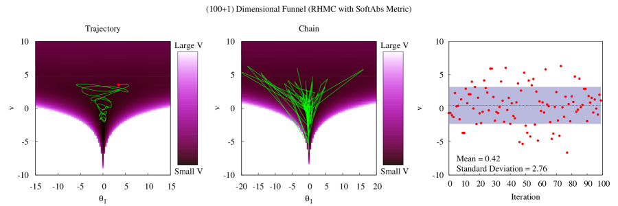
Of course, the utility of Riemannian Hamiltonian Monte Carlo is dependent on the choice of the metric $\Sigma\!\left(q\right)$. To optimize the position-dependent corrections we want a metric that leaves the target distribution locally isotropic, motivating a metric resembling the Hessian of the target distribution. Unfortunately the Hessian isn’t sufficiently well-behaved to serve as a metric itself; in general, it is not even guaranteed to be positive-definite. The Hessian can be manipulated into a well-behaved form, however, by applying the SoftAbs transformation, and the resulting SoftAbs metric Betancourt:2013a admits a generic but efficient Riemannian Hamiltonian Monte Carlo implementation (Figure 10, 11).

Figure 10: Although the variation in the potential energy, $V$, is still limited by the variation in the kinetic energy, $T$, the introduction of the log determinant term in Riemannian Hamiltonian Monte Carlo allows the kinetic energy sufficiently large variation that the potential is essentially unconstrained in practice.

Figure 11: Without being limited to small variations in the potential energy, Riemannian Hamiltonian Monte Carlo with the SoftAbs metric admits transitions that expire the entirety of the funnel distribution, resulting in nearly independent transitions, and drastically smaller autocorrelations (compare with Figure 7, noting the different number of iterations).

IV Example

To see the advantage of Hamiltonian Monte Carlo over algorithms that explore with a random walk, consider the one-way normal model (2) with 800 latent $\theta_{i}$ and a constant measurement error, $\sigma_{i}=\sigma$ across all nodes. The latent parameters are taken to be $\mu=8$ and $\tau=3$, with the $\theta_{i}$ and $y_{i}$ randomly sampled in turn with $\sigma=10$. To this generative likelihood we add weakly-informative priors,

$$\pi\!\left(\mu\right) =\mathcal{N}\!\left(0,5^{2}\right)$$

$$\pi\!\left(\tau\right) =\text{Half-Cauchy}\!\left(0,2.5\right).$$

All sampling is done on a fully unconstrained space, in particular the latent $\tau$ is transformed into $\lambda=\log\tau$.

Noting the results of Figure 8, the nominal centered parameterization,

$$y_{i} \sim\mathcal{N}\!\left(\theta_{i},\sigma_{i}^{2}\right)$$

$$\theta_{i} \sim\mathcal{N}\!\left(\mu,\tau^{2}\right),\mbox{ for }i=1,\dots,800,$$

should yield inferior performance to the non-centered parameterization,

$$y_{i} \sim\mathcal{N}\!\left(\tau\vartheta_{i}+\mu,\sigma_{i}^{2}\right)$$ (3)

$$\vartheta_{i} \sim\mathcal{N}\!\left(0,1\right),\mbox{ for }i=1,\dots,800;$$ (4)

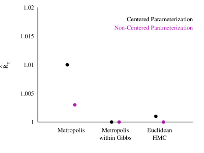
in order to not overestimate the success of Hamiltonian Monte Carlo we include both. For both parameterizations, we fit Random Walk Metropolis, Metropolis-within-Gibbs, and Euclidean Hamiltonian Monte Carlo with a diagonal metric to the generated data. The step size parameter in each case was tuned to be as large as possible whilst still yielding consistent estimates with a baseline sample generated from running Euclidean Hamiltonian Monte Carlo with a large target acceptance probability (Figure 12).

Although the pathologies of the centered parameterization penalize all three algorithms, Euclidean Hamiltonian Monte Carlo proves to be at least an order-of-magnitude more efficient than both Random Walk Metropolis and the Gibbs sampler. The real power of Hamiltonian Monte Carlo, however, is revealed when those penalties are removed in the non-centered parameterization (Table 1).

Most importantly, the advantage of Hamiltonian Monte Carlo scales with increasing dimensionality of the model. In the most complex models that populate the cutting edge of applied statistics, Hamiltonian Monte Carlo is not just the most convenient solution, it is often the only practical solution.

Figure 12: In order to ensure valid comparisons, each sampling algorithm was optimized but only so long as the resulting estimates were consistent with each other.

Algorithm	Parameterization	Step Size	Average	Time	Time/ESS
			Acceptance	(s)	(s)
			Probability
Metropolis	Centered	$5.00\cdot 10^{-3}$	0.822	$4.51\cdot 10^{4}$	1220
Gibbs	Centered	1.50	0.446	$9.54\cdot 10^{4}$	297
EHMC	Centered	$1.91\cdot 10^{-2}$	0.987	$1.00\cdot 10^{4}$	16.2
Metropolis	Non-Centered	0.0500	0.461	398	1.44
Gibbs	Non-Centered	2.00	0.496	817	1.95
EHMC	Non-Centered	0.164	0.763	154	$\mathbf{2.94\cdot 10^{-2}}$

Table 1: Euclidean Hamiltonian Monte Carlo significantly outperforms both Random Walk Metropolis and the Metropolis-within-Gibbs sampler for both parameterizations of the one-way normal model. The difference is particularly striking for the more efficient non-centered parameterization that would be used in practice.

V Conclusion

By utilizing the local curvature of the target distribution, Hamiltonian Monte Carlo provides the efficient exploration necessary for learning from the complex hierarchical models of interest in applied problems. Whether using Euclidean Hamiltonian Monte Carlo with careful parameterizations or Riemannian Hamiltonian Monte Carlo with the SoftAbs metric, these algorithms admit inference whose performance scales not just with the size of the hierarchy but also with the complexity of local distributions, even those that may not be amenable to analytic manipulation.

The immediate drawback of Hamiltonian Monte Carlo is increased difficulty of implementation: not only does the algorithm require non-trivial tasks such as the the integration of Hamilton’s equations, the user must also specify the derivatives of the target distribution. The inference engine Stan Stan:2013 removes these burdens, providing not only a powerful probabilistic programming language for specifying the target distribution and a high performance implementation of Hamiltonian evolution but also state-of-the-art automatic differentiation techniques to compute the derivatives without any user input. Through Stan, users can build, test, and run hierarchical models without having to compromise for computational constraints.

VI Acknowledgements

We are indebted to Simon Byrne, Bob Carpenter, Michael Epstein, Andrew Gelman, Yair Ghitza, Daniel Lee, Peter Li, Sam Livingstone, and Anne-Marie Lyne for many fruitful discussions as well as invaluable comments on the text. Michael Betancourt is supported under EPSRC grant EP/J016934/1 and Mark Girolami is an EPSRC Research Fellow under grant EP/J016934/1.

Appendix A Stan Models

One advantage of Stan is the ability to easily share and reproduce models. Here we include all models used in the tests above; results can be reproduced using the development branch https://github.com/stan-dev/stan/tree/f5df6e139df606c03bf02f4ff99d2341c15f73cd which will be incorporated into Stan v.2.1.0.

Funnel

Model

transformed data {
  int<lower=0> J;
  J <- 25;
}
parameters {
  real theta[J];
  real v;
}
model {
  v ~ normal(0, 3);
  theta ~ normal(0, exp(v/2));
}

Generate One-Way Normal Pseudo-data

Model

transformed data {
  real mu;
  real<lower=0> tau;

  real alpha;
  int N;

  mu <- 8;
  tau <- 3;

  alpha <- 10;
  N <- 800;

}

parameters {
  real x;
}

model {
  x ~ normal(0, 1);
}

generated quantities {
  real mu_print;
  real tau_print;

  vector[N] theta;
  vector[N] sigma;
  vector[N] y;

  mu_print <- mu;
  tau_print <- tau;

  for (i in 1:N) {
    theta[i] <- normal_rng(mu, tau);
    sigma[i] <- alpha;
    y[i] <- normal_rng(theta[i], sigma[i]);
  }

}

Configuration

./generate_big_psuedodata sample num_warmup=0
num_samples=1 random seed=48383823
output file=samples.big.csv

One-Way Normal (Centered)

Model

data {
  int<lower=0> J;
  real y[J];
  real<lower=0> sigma[J];
}

parameters {
  real mu;
  real<lower=0> tau;
  real theta[J];
}

model {
  mu ~ normal(0, 5);
  tau ~ cauchy(0, 2.5);
  theta ~ normal(mu, tau);
  y ~ normal(theta, sigma);
}

Configuration

./n_schools_cp sample num_warmup=100000 num_samples=1000000
thin=1000 adapt delta=0.999 algorithm=hmc engine=nuts
max_depth=20 random seed=39457382 data file=big_schools.dat
output file=big_schools_ehmc_cp.csv

One-Way Normal (Non-Centered)

Model

data {
  int<lower=0> J;
  real y[J];
  real<lower=0> sigma[J];
}

parameters {
  real mu;
  real<lower=0> tau;
  real var_theta[J];
}

transformed parameters {
  real theta[J];
  for (j in 1:J) theta[j] <- tau * var_theta[j] + mu;
}

model {
  mu ~ normal(0, 5);
  tau ~ cauchy(0, 2.5);
  var_theta ~ normal(0, 1);
  y ~ normal(theta, sigma);
}

Configuration (Baseline)

./n_schools_ncp sample num_warmup=5000 num_samples=100000
adapt delta=0.99 random seed=466772400 data file=big_schools.dat
output file=big_schools_baseline.csv

Configuration (Nominal)

./n_schools_ncp sample num_warmup=5000 num_samples=50000
adapt delta=0.8 random seed=95848382 data file=big_schools.dat
output file=big_schools_ehmc_ncp.csv

References

- (1) A. Gelman et al., Bayesian Data Analysis, 3rd ed. (CRC Press, London, 2013).
- (2) R. Neal, Annals of statistics , 705 (2003).
- (3) J. C. Pinheiro and D. M. Bates, Linear mixed-effects models: basic concepts and examples (Springer, 2000).
- (4) S. Rabe-Hesketh and A. Skrondal, Multilevel and longitudinal modelling using Stata (STATA press, 2008).
- (5) H. Rue, S. Martino, and N. Chopin, Journal of the royal statistical society: Series b (statistical methodology) 71, 319 (2009).
- (6) C. P. Robert, G. Casella, and C. P. RobertMonte Carlo statistical methods Vol. 58 (Springer New York, 1999).
- (7) C. Liu, D. B. Rubin, and Y. N. Wu, Biometrika 85, 755 (1998).
- (8) J. S. Liu and Y. N. Wu, Journal of the American Statistical Association 94, 1264 (1999).
- (9) A. Gelman, D. A. Van Dyk, Z. Huang, and J. W. Boscardin, Journal of Computational and Graphical Statistics 17 (2008).
- (10) O. Papaspiliopoulos, G. O. Roberts, and M. Sköld, Statistical Science , 59 (2007).
- (11) S. Duane, A. Kennedy, B. J. Pendleton, and D. Roweth, Physics Letters B 195, 216 (1987).
- (12) R. Neal, Mcmc using hamiltonian dynamics, in Handbook of Markov Chain Monte Carlo, edited by S. Brooks, A. Gelman, G. L. Jones, and X.-L. Meng, CRC Press, New York, 2011.
- (13) M. Betancourt and L. C. Stein, arXiv preprint arXiv:1112.4118 (2011).
- (14) M. Betancourt, ArXiv e-prints (2013), 1304.1920.
- (15) M. D. Hoffman and A. Gelman, ArXiv e-prints (2011), 1111.4246.
- (16) E. Hairer, C. Lubich, and G. WannerGeometric numerical integration: structure-preserving algorithms for ordinary differential equations Vol. 31 (Springer, 2006).
- (17) A. Beskos, N. Pillai, G. Roberts, J. Sanz-Serna, and S. Andrew, Bernoulli (forthcoming) (2013).
- (18) A. Gelman and D. B. Rubin, Statistical science , 457 (1992).
- (19) Stan Development Team, Stan Modeling Language User’s Guide and Reference Manual, Version 2.0, 2013.
- (20) Stan Development Team, Stan: A c++ library for probability and sampling, version 2.0, 2013.
- (21) M. Girolami and B. Calderhead, Journal of the Royal Statistical Society: Series B (Statistical Methodology) 73, 123 (2011).
- (22) M. Betancourt, A general metric for riemannian hamiltonian monte carlo, in First International Conference on the Geometric Science of Information, edited by Nielsen, F. and Barbaresco, F., , Lecture Notes in Computer Science Vol. 8085, Springer, 2013.