Mean-field yrast spectrum and persistent currents in a two-component Bose gas with interaction asymmetry

Abstract

We analyze the mean-field yrast spectrum of a two-component Bose gas in the ring geometry with arbitrary interaction asymmetry. Of particular interest is the possibility that the yrast spectrum develops local minima at which persistent superfluid flow can occur. By analyzing the mean-field energy functional, we show that local minima can be found at plane-wave states and arise when the system parameters satisfy certain inequalities. We then go on to show that these plane-wave states can be yrast states even when the yrast spectrum no longer exhibits a local minimum. Finally, we obtain conditions which establish when the plane-wave states cease to be yrast states. Specific examples illustrating the roles played by the various interaction asymmetries are presented.

I Introduction

The experimental realization of annular trapping potentials gupta05 ; ryu07 ; sherlock11 has recently led to the observation of persistent superfluid flow in a multiply-connected geometry ryu07 ; ramanathan11 ; moulder12 ; beattie13 . The question of the stability of these superfluid currents is a complex matter and depends on the nature of the dynamical excitations available to the system. The current consensus is that stability is limited by the penetration of vortices through the edge of the superfluid with a concomitant change in the phase of the superfluid order parameter. Several theoretical studies support this scenario anglin01 ; dubessy12 ; yakimenko13 ; abad14 ; yakimenko15 .

However, underlying these dynamical instabilities is the inherent metastability of the superfluid system. As emphasized by Bloch Bloch , this metastability is revealed through the energy of the superfluid as a function of its angular momentum, its so-called yrast spectrum Mottelson . In this paper, we investigate the yrast spectrum of a two-component Bose gas in the ring geometry. Specifically, we have in mind the situation in which the atoms are confined to a torus where the transverse confinement is so tight that the system is effectively one-dimensional. When the two species have equal masses $M$, it can be shown quite generally Smyrnakis1 ; Anoshkin that the yrast spectrum takes the form

$$E_{0}(L)=\frac{L^{2}}{2M_{T}R^{2}}+e_{0}(L),$$ (1)

where $R$ is the radius of the ring, $L$ is the total angular momentum and $M_{T}=MN$ is the total mass of the system. Here, $N=N_{A}+N_{B}$ is the total number of atoms of type $A$ and $B$. The function $e_{0}(L)$ has inversion symmetry and possesses the periodicity property $e_{0}(L+N\hbar)=e_{0}(L).$

The above properties of the yrast spectrum are independent of the detailed nature of the inter-particle interactions Anoshkin . For contact interactions, the interactions can be characterised by the dimensionless parameters $\gamma_{ss^{\prime}}$ where the subscripts $s$ and $s^{\prime}$ take on the values $A$ and $B$. (A detailed definition of these interaction parameters is given in Sec. II.) However, as shown in several previous studies Smyrnakis1 ; Smyrnakis2 ; Smyrnakis3 ; Anoshkin ; Wu , the mean-field yrast spectrum of the two-component system, with the added restriction that all interaction strengths have a common value $\gamma$, exhibits two additional properties. First, the part of the spectrum in the fundamental range $0\leq l\leq 1/2$, where $l=L/N\hbar$, is not in general an analytic function of the (dimensionless) angular momentum per particle. In particular, the derivative of the spectrum is found to exhibit discontinuities at $l=qx_{B}$, where $x_{B}=N_{B}/N$ is the minority concentration and $q=1,2,...,k$. The number of discontinuities $k$ depends on the two relevant parameters of the model, namely $\gamma$ and $x_{B}$. More specifically, it was established that $k$ derivative discontinuities occur when the coordinate $(\gamma,x_{B})$ lies within a region bounded by the two critical curves $x_{B}(\gamma,k)$ and $x_{B}(\gamma,k+1)$ in the $\gamma$-$x_{B}$ plane Wu . These curves are illustrated by the solid lines in Fig. 1 for $k=2,...,4$. Importantly, the point of non-analyticity, $l=qx_{B}$, is associated with the condensate wavefunctions having a plane-wave form, $(\psi_{A},\psi_{B})=(\phi_{0},\phi_{q})$, where $\phi_{q}=e^{iq\theta}/\sqrt{2\pi}$. As a result, the relevant critical $x_{B}(\gamma,k)$ curves in Fig. 1 can also be viewed as defining the regions within which plane-wave yrast states emerge. For values of $l$ other than these special values, the yrast state is in general a soliton state.

Now, because of the periodicity and inversion symmetry of $e_{0}(L)$, a derivative discontinuity at $l=kx_{B}$ implies discontinuities at $l=\mu\pm kx_{B}$ as well, where $\mu$ is any non-zero integer. The yrast states at these angular momenta are $(\psi_{A},\psi_{B})=(\phi_{\mu},\phi_{\mu\pm k})$. The second important property of the yrast spectrum concerns a subset of such non-analytic points, namely those at $l=k-kx_{B}=kx_{A}$. It can be shown Wu that the yrast spectrum has local minima at these angular momenta (and only these from all possible $l=\mu\pm kx_{B}$) for any integer $k$ provided $\gamma$ exceeds the critical interaction strength

$$\gamma_{{\rm cr},k}=\frac{4k^{2}-1}{2(1-4x_{B}k^{2})}.$$ (2)

This expression provides another set of critical $x_{B}(\gamma,k)$ curves, which are indicated by the dashed lines in Fig. 1. Since a local minimum at $l=k-kx_{B}$ necessarily implies that the corresponding state $(\psi_{A},\psi_{B})=(\phi_{k},\phi_{0})$ is already an yrast state, $\gamma>\gamma_{{\rm cr},k}$ is thus a sufficient, but not necessary, condition for the existence of plane-wave yrast states. This is reflected in the fact that the dashed curves in Fig. 1 are displaced to the right of the solid curves; with increasing $\gamma$ for a fixed $x_{B}$, one first crosses a solid curve at which point some plane-wave state becomes an yrast state, and then the dashed curve beyond which this plane-wave state is a local minimum. The existence of an energy minimum is of particular significance since, as argued by Bloch Bloch , it implies the possibility of persistent superfluid flow. Thus, the condition $\gamma>\gamma_{{\rm cr},k}$ can be taken as the stability condition for persistent currents at the angular momentum $l=k-kx_{B}$.

Figure 1: The solid lines are critical curves for the emergence of plane-wave yrast states. In the region bounded by $x_{B}(\gamma,k)$ and $x_{B}(\gamma,k+1)$, the plane-wave states $(\phi_{0},\phi_{q})$, with $q=1,...,k$ are yrast states. The critical curve for $k=1$, $x_{B}(\gamma,1)=0.5$, is not shown. The dashed lines are critical curves defining the regions in which the $(\phi_{k},\phi_{0})$ state supports persistent currents.

The above conclusions, pertaining to a system with symmetrical interaction strengths, were reached with aid of analytic soliton solutions to the coupled Gross-Pitaevskii equations, from which the full yrast spectrum could be determined Wu . These conclusions were confirmed by Smyrnakis et al. Smyrnakis14 using an alternative approach. Since the symmetrical model is rather special, it is unclear whether the aforementioned properties of the mean-field yrast spectrum remain valid for the asymmetrical model in which the interparticle interactions take on different values. This is the main question to be addressed in this paper. To answer it we adopt the strategy, motivated by the symmetrical model, of examining the mean-field energy functional in the vicinity of plane-wave states. Even though analytic soliton solutions are not known for the asymmetrical model, we are able to use a perturbative analysis to determine the general behaviour of the energy functional near plane-wave states and obtain critical conditions analogous to those displayed in Fig. 1. Since all of the results for the symmetrical model are recovered by this approach, we are confident that the conditions we derive do in fact determine the stability of persistent currents in the asymmetrical model.

The rest of the paper is organized as follows. In Sec. II, we derive inequalities involving the system parameters which establish whether a given plane-wave state is a local minimum of the Gross-Pitaevskii energy functional. Such a state has a specific angular momentum $l$. We then argue that the lowest-energy plane-wave state having this angular momentum is a global minimum if the inequalities for this state are satisfied and, hence, is an yrast state. These predictions are then checked against known limiting situations, including that of the symmetric model. In Sec. III we then analyze in more detail the behaviour of the yrast spectrum in the vicinity of a plane-wave state corresponding to a global minimum. We first establish that the yrast spectrum has a derivative discontinuity at the angular momentum $l$ of this state. The instability of persistent currents at this angular momentum is then signalled by the critical condition that one of the slopes of the yrast spectrum vanishes. At this point, the plane-wave state is no longer a local minimum. We then obtain a subsequent critical condition for the disappearance of the derivative discontinuity. This condition provides a bound for the plane-wave state to be an yrast state. We conclude this section with some applications of these critical conditions in the determination of plane-wave yrast states. The main results of the paper are summarized in the final section.

II Local minima of the energy functional at plane-wave states

The system of interest is a two-species Bose gas consisting of $N_{A}$ particles of type $A$ and $N_{B}$ particles of type $B$ confined to a ring of radius $R$. We assume that the two species have the same mass $M$. Within a mean-field description, the condensate wave functions $\psi_{A}$ and $\psi_{B}$ define the Gross-Pitaevskii (GP) energy functional (in units of $N\hbar^{2}/2MR^{2}$)

$$\bar{E}[\psi_{A},\psi_{B}]= \int_{0}^{2\pi}d\theta\left(x_{A}\left|\frac{d\psi_{A}}{d\theta}\right|^{2}+x_{B}\left|\frac{d\psi_{B}}{d\theta}\right|^{2}\right)+x_{A}^{2}\pi\gamma_{AA}\int_{0}^{2\pi}d\theta|\psi_{A}(\theta)|^{4}+x_{B}^{2}\pi\gamma_{BB}\int_{0}^{2\pi}d\theta|\psi_{B}(\theta)|^{4}$$

$$+2x_{A}x_{B}\pi\gamma_{AB}\int_{0}^{2\pi}d\theta|\psi_{A}(\theta)|^{2}|\psi_{B}(\theta)|^{2},$$ (3)

where the dimensionless interaction parameters are defined as $\gamma_{ss^{\prime}}=U_{ss^{\prime}}NMR^{2}/\pi\hbar^{2}$ with $N=N_{A}+N_{B}$. For the most part, we are concerned with repulsive interactions, $\gamma_{ss^{\prime}}>0$. With the condensate wave functions normalized according to

$$\int_{0}^{2\pi}d\theta|\psi_{s}(\theta)|^{2}=1,$$ (4)

the energy per particle defined in Eq. (3) depends on the particle numbers only through the concentrations $x_{s}=N_{s}/N$.

Our ultimate objective is the determination of the yrast spectrum which is defined by the lowest energy of the system as a function of the angular momentum. In units of $N\hbar$, the total angular momentum of the system is given by

$$\bar{L}[\psi_{A},\psi_{B}]=\sum_{s}\frac{x_{s}}{i}\int_{0}^{2\pi}d\theta\psi_{s}^{*}(\theta)\frac{\partial}{\partial\theta}\psi_{s}(\theta).$$ (5)

The minimization of Eq. (3) with the constraint $\bar{L}[\psi_{A},\psi_{B}]=l$ gives the yrast energy

$$\bar{E}_{0}(l)=l^{2}+e_{0}(l),$$ (6)

where $e_{0}(l)$ is an even function of $l$ with the periodicity property $e_{0}(l+n)=e_{0}(l)$, $n$ being an arbitrary integer Anoshkin . As a result of these properties, the yrast spectrum is completely determined by the behaviour of $e_{0}(l)$ in the interval $0\leq l\leq 1/2$. If a point $l_{0}$ in this interval is a point of nonanalyticity of $e_{0}(l)$, then the points $n\pm l_{0}$ for any integer $n$ are points of nonanalyticity of $\bar{E}_{0}(l)$. As we shall show, these points occur at plane-wave yrast states.

We are therefore led to an investigation of the behaviour of the GP energy functional in the vicinity of some arbitrary plane-wave state $(\phi_{\mu},\phi_{\nu})$. As discussed in the Introduction, the conditions for which such a state is an yrast state are known in the case of the symmectrical model. There it is found that the yrast spectrum exhibits a derivative discontinuity at the angular momentum corresponding to this state, namely at

$$l=\mu x_{A}+\nu x_{B}\equiv\mu+kx_{B},$$ (7)

where $k=\nu-\mu$. Furthermore, the criteria for the yrast spectrum exhibiting a local minimum at one of these angular momenta is also known. The question we wish to address in this paper is the extent to which such states can be yrast states in the asymmetrical model.

For the $(\phi_{\mu},\phi_{\nu})$ plane-wave state we have

$$\bar{E}[\phi_{\mu},\phi_{\nu}]=\bar{E}_{\rm int}+l^{2}+x_{A}x_{B}k^{2},$$ (8)

with

$$\bar{E}_{\rm int}=\frac{1}{2}(x_{A}^{2}\gamma_{AA}+2x_{A}x_{B}\gamma_{AB}+x_{B}^{2}\gamma_{BB}).$$ (9)

All such plane-wave states have the same interaction energy $\bar{E}_{\rm int}$ but a kinetic energy which depends on the parameters $\mu$ and $\nu$ or alternatively, $l$ and $k$.

In searching for the minimum energy plane-wave state of a given angular momentum $l$, it is useful to note that $x_{B}=N_{B}/N$ is in general a rational number which we denote by

$$x_{B}=\frac{p}{q}$$ (10)

where $p$ and $q$ are positive integers having no common divisor. One can easily check that the plane-wave states ($\phi_{\mu^{\prime}},\phi_{\mu^{\prime}+k^{\prime}}$) defined by the parameters

$$\mu^{\prime}=\mu+mp,\quad k^{\prime}=k-mq,$$ (11)

where $m=0,\,\pm 1,\,\pm 2,...$, all have the same angular momentum $l$. In view of Eq. (8), the lowest energy state from this infinite set is obtained for the smallest value of $|k^{\prime}|$. This value of $k^{\prime}$ will be found in the range

$$-\left[\frac{q}{2}\right]\leq k^{\prime}\leq\left[\frac{q}{2}\right]$$ (12)

where $[q/2]$ is the largest integer less than or equal to $q/2$, that is, the floor of $q/2$. It is worth noting that the allowed angular momentum values of the plane-waves states take the form $l=Q/q$, where $Q$ is an arbitrary integer. Of course, when the restriction $0\leq l\leq 1/2$ is imposed, one need only consider $Q=0,1,...,[q/2]$.

Let us now consider the plane-wave state ($\phi_{\mu},\phi_{\mu+k}$) with $k$ restricted to the range given by Eq. (12). If $q$ is odd, the set of $k$ values in this range corresponds to a complete residue system modulo $q$. Thus, when each possible value of $k$ in this range is paired with each possible value of $\mu$, all possible values of the angular momentum $l$ are generated without duplication. As a result, the value of $k$ which minimizes the energy for a given $l$ is unique. The situation for even $q$ is slightly different since $-[q/2]$ and $[q/2]$ are congruent and there are two plane-wave states, namely ($\phi_{\mu}$, $\phi_{\mu+q/2}$) and ($\phi_{\mu+p}$, $\phi_{\mu+p-q/2}$), which have the same angular momentum and energy. Thus, one cannot decide which of these two states is a potential yrast state at this particular angular momentum. However, we do have a prescription for selecting, from all possible plane-wave states having the same $l$, the specific state(s) that are potential yrast states.

We note that if $x_{B}$ is treated as a continuous variable, it will of course take on irrational values. In this case, no two plane-wave states will have the same angular momentum and the complexities associated with rational $x_{B}$ are avoided. However, whenever $x_{B}$ takes on a rational value, the above considerations will once again apply.

Although our analysis could be restricted to the plane-wave states with $k$ in the range specified by Eq. (12), it is more convenient to consider in the following the GP energy functional in the vicinity of an arbitrary $(\phi_{\mu},\phi_{\nu})$ plane-wave state. To be specific, our goal is to establish the conditions for which the energy functional will exhibit a local minimum at this state. To this end, we consider states $(\psi_{A},\psi_{B})$ which deviate slightly from $(\phi_{\mu},\phi_{\nu})$, viz.

$$\psi_{A}=\phi_{\mu}+\delta\psi_{A},\hskip 28.45274pt\psi_{B}=\phi_{\nu}+\delta\psi_{B},$$ (13)

where the deviations are expressed in the form

$$\delta\psi_{A} =\delta c_{\mu}\phi_{\mu}+\sum\limits_{m>0}\left(\delta c_{\mu+m}\phi_{\mu+m}+\delta c_{\mu-m}\phi_{\mu-m}\right),$$ (14)

$$\delta\psi_{B} =\delta d_{\nu}\phi_{\nu}+\sum\limits_{m>0}\left(\delta d_{\nu+m}\phi_{\nu+m}+\delta d_{\nu-m}\phi_{\nu-m}\right).$$ (15)

The normalization of these states implies

$$|1+\delta c_{\mu}|^{2}+\sum_{n\neq\mu}|\delta c_{n}|^{2} =1$$ (16)

$$|1+\delta d_{\nu}|^{2}+\sum_{n\neq\nu}|\delta d_{n}|^{2} =1.$$ (17)

These relations indicate, for example, that $|1+\delta c_{\mu}|^{2}\leq 1$ and $\sum_{n\neq\mu}|\delta c_{n}|^{2}\leq 1$. Alternatively, these normalization conditions can be expressed as

$$\delta c_{\mu}+\delta c_{\mu}^{*}+\sum_{n}|\delta c_{n}|^{2} =0$$ (18)

$$\delta d_{\nu}+\delta d_{\nu}^{*}+\sum_{n}|\delta d_{n}|^{2} =0.$$ (19)

Substituting Eq. (13) into Eq. (3) and eliminating $\delta c_{\mu}$ and $\delta d_{\nu}$ by means of Eqs. (18) and (19), we find that the change in energy to second order in the deviations is given by

$$\delta\bar{E}[\psi_{A},\psi_{B}] =\bar{E}[\psi_{A},\psi_{B}]-\bar{E}[\phi_{\mu},\phi_{\nu}]$$

$$\simeq\sum_{m>0}{\bf v}^{\dagger}_{m}{\mathcal{H}}_{m}{\bf v}_{m},$$ (20)

where ${\bf v}_{m}=(\delta c_{\mu-m}\,\,\delta c^{*}_{\mu+m}\,\,\delta d_{\nu-m}\,\,\delta d^{*}_{\nu+m})^{\rm T}$ and

$$\mathcal{H}_{m}=\left(\begin{array}[]{cccc}x_{A}(x_{A}\gamma_{AA}+m^{2}-2\mu m)&x_{A}^{2}\gamma_{AA}&x_{A}x_{B}\gamma_{AB}&x_{A}x_{B}\gamma_{AB}\\ x_{A}^{2}\gamma_{AA}&x_{A}(x_{A}\gamma_{AA}+m^{2}+2\mu m)&x_{A}x_{B}\gamma_{AB}&x_{A}x_{B}\gamma_{AB}\\ x_{A}x_{B}\gamma_{AB}&x_{A}x_{B}\gamma_{AB}&x_{B}(x_{B}\gamma_{BB}+m^{2}-2\nu m)&x_{B}^{2}\gamma_{BB}\\ x_{A}x_{B}\gamma_{AB}&x_{A}x_{B}\gamma_{AB}&x_{B}^{2}\gamma_{BB}&x_{B}(x_{B}\gamma_{BB}+m^{2}+2\nu m)\end{array}\right).$$ (21)

We thus see that the change in energy is a quadtratic form.

If the matrices $\mathcal{H}_{m}$ are all positive definite, the energy $\bar{E}[\phi_{\mu},\phi_{\nu}]$ is a local minimum in the function space defined by $\psi_{A}$ and $\psi_{B}$. According to Sylvester’s criterion Gelfand , positive-definiteness is assured if all the leading principal minors of $\mathcal{H}_{m}$ are positive, namely

$$x_{A}\gamma_{AA}+m^{2}-2\mu m>0,$$ (22)

$$2x_{A}\gamma_{AA}+m^{2}-4\mu^{2}>0,$$ (23)

$$\left(2x_{A}\gamma_{AA}+m^{2}-4\mu^{2}\right)\left(x_{B}\gamma_{BB}+m^{2}-2\nu m\right)-2x_{A}x_{B}\gamma_{AB}^{2}>0,$$ (24)

$$\left(2x_{A}\gamma_{AA}+m^{2}-4\mu^{2}\right)\left(2x_{B}\gamma_{BB}+m^{2}-4\nu^{2}\right)-4x_{A}x_{B}\gamma^{2}_{AB}>0.$$ (25)

It is straighforward to show that Eq. (23) implies Eq. (22); likewise, Eq. (25) together with Eq. (23) implies Eq. (24). Thus, Eqs. (23) and (25) are the fundamental inequalities determining the positive-definiteness of ${\cal H}_{m}$. Furthermore, these inequalities are satisfied for all $m$ if they are satisfied for $m=1$. We thus see that the inequalities

$$2x_{A}\gamma_{AA}+1-4\mu^{2}>0,$$ (26)

$$\left(2x_{A}\gamma_{AA}+1-4\mu^{2}\right)\left(2x_{B}\gamma_{BB}+1-4\nu^{2}\right)-4x_{A}x_{B}\gamma^{2}_{AB}>0$$ (27)

are the necessary and sufficient conditions for $(\phi_{\mu},\,\phi_{\nu})$ being a local minimum in the function space. It is important to note that, although the state $(\phi_{\mu},\,\phi_{\nu})$ has the angular momentum $l=\mu x_{A}+\nu x_{B}$, the variations in Eq. (13) allow for deviations of the angular momentum from this value. In other words, the local minimum that we are finding is not constrained by the angular momentum $l$; the local minimum exists for arbitrary variations of the condensate wave functions about the plane-wave state of interest.

On the other hand, it is possible to consider variations which are further constrained (apart from normalization) by the angular momentum $l=\mu x_{A}+\nu x_{B}$; such states define a hypersurface in function space. The state $(\phi_{\mu},\,\phi_{\nu})$ lies on this surface and, if the inequalities in Eqs. (26) and (27) are satisfied, its energy is lower than that of any other state in its vicinity on the hypersurface. If this state were in fact a global minimum on the hypersurface, it would be, by definition, an yrast state. Since the specific plane-wave state $(\phi_{\mu},\phi_{\nu})$, where $\nu=\mu+k$ with $k$ restricted to the range in Eq. (12), has the lowest energy of all the plane-wave states having the same angular momentum, it is clearly a candidate for being the global minimum. In the Appendix, we show that conditions exist for which such a state is assured to be a global minimum on the $l=\mu+kx_{B}$ hypersurface. We now make the stronger assumption that this specific plane-wave state is a global minimum when the inequalities in Eqs. (26) and (27) are satisfied, and is hence an yrast state. As we shall show, this assumption is consistent with the results of the symmetric model and, for reasons of continuity, would be expected to continue holding as the interaction parameters gradually become asymmetrical. Furthermore, the inequalities in Eqs. (26) and (27) also ensure that the energy increases as one moves away from $(\phi_{\mu},\phi_{\nu})$ in directions of either increasing or decreasing angular momenta. According to the Bloch criterion, this would imply that persistent currents are stable at the $l=\mu+kx_{B}$ angular momentum point of the yrast spectrum. We now consider some special cases in order to make contact with earlier work. Unless stated otherwise, the $\mu$ and $\nu$ indices will henceforth refer to plane-wave states for which the difference $k=\nu-\mu$ is restricted to the range in Eq. (12).

II.1 Case 1: $\mu=\nu=n$

This case corresponds to integral angular momenta, $l=n$. Eq. (27) then reduces to

$$\left(x_{A}\gamma_{AA}-\frac{4n^{2}-1}{2}\right)\left(x_{B}\gamma_{BB}-\frac{4n^{2}-1}{2}\right)>x_{A}x_{B}\gamma^{2}_{AB}.$$ (28)

This together with Eq. (26) implies

$$x_{A}\gamma_{AA}+x_{B}\gamma_{BB}>4n^{2}-1.$$ (29)

These are the two inequalities given in Ref. Anoshkin that establish the stability of persistent currents at integral values of $l$.

For $n=0$, Eq. (28) reduces to

$$\left(x_{A}\gamma_{AA}+\frac{1}{2}\right)\left(x_{B}\gamma_{BB}+\frac{1}{2}\right)>x_{A}x_{B}\gamma^{2}_{AB}$$ (30)

This is the condition for energetic or dynamic stability and ensures that the uniform state $(\phi_{0},\phi_{0})$ is stable against phase separation. This state gives the absolute minimum of the GP energy functional, and by virtue of the periodicity of $e_{0}(l)$, the states $(\phi_{n},\phi_{n})$ with integral angular momentum $l=n$ are all yrast states. It is thus clear from a consideration of this special case that the inequalities in Eqs. (26) and (27) do in fact define a global minimum on the $l=n$ hypersurface.

If we now consider the special case $\gamma_{AA}\gamma_{BB}=\gamma_{AB}^{2}$, the inequality in Eq. (28) for $n\neq 0$ reduces to

$$x_{A}\gamma_{AA}+x_{B}\gamma_{BB}<\frac{1}{2}(4n^{2}-1).$$ (31)

This inequality is incompatible with Eq. (29) which implies that the $(\phi_{n},\phi_{n})$ state cannot be a local minimum for these interaction parameters. However, if Eq. (30) is satisfied, this state is still an yrast state. Thus, a local minimum in function space is not a necessary condition for the plane-wave state being an yrast state. In the following section we will show that the absence of a local minimum in function space also implies the lack of a local minimum in the yrast spectrum and the absence of persistent currents. As explained in Ref. Anoshkin , the physical reason for the absence of persistent currents when $\gamma_{AA}\gamma_{BB}=\gamma_{AB}^{2}$ is that the Bogoliubov excitations exhibit a particle-like dispersion which destabilizes superfluid flow.

II.2 Case 2: $\mu\neq\nu$; $\gamma_{AA}\gamma_{BB}=\gamma_{AB}^{2}$

In this case, the inequality in Eq. (27) reduces to

$$(1-4\nu^{2})(2x_{A}\gamma_{AA}+1-4\mu^{2})+2x_{B}\gamma_{BB}(1-4\mu^{2})>0.$$ (32)

If $\mu=0$, this inequality implies

$$\nu^{2}<\frac{1+2x_{A}\gamma_{AA}+2x_{B}\gamma_{BB}}{4(1+2x_{A}\gamma_{AA})}.$$ (33)

The values of $\nu$ satisfying this inequality depend on the values of the parameters $x_{A}$, $\gamma_{AA}$ and $\gamma_{BB}$. If $\mu\geq 1$, we have $(1-4\mu^{2})<0$. Thus in view of Eq. (26), the inequality in Eq. (32) can only be satisfied if $\nu=0$. We have thus established that local minima can occur at the states $(\phi_{\mu},\phi_{0})$ with angular momenta $l=\mu x_{A}$ or at $(\phi_{0},\phi_{\nu})$ with angular momenta $l=\nu x_{B}$. In this latter case, however, the range of $\nu$ is limited by the inequality in Eq. (33).

In the symmetric model with $\gamma_{AA}=\gamma_{BB}=\gamma_{AB}=\gamma$, the only possible value of $\nu$ in Eq. (33) is zero if we take $A$ to be the majority component ($x_{A}>1/2$). Thus local minima can only occur for the $(\phi_{\mu},\phi_{0})$ states in this case. Furthermore, Eq. (32) gives

$$\gamma>\frac{4\mu^{2}-1}{2(1-4x_{B}\mu^{2})}.$$ (34)

This is precisely the condition for persistent currents to occur at $l=\mu x_{A}$ found in Ref. Wu using the explicit soliton solutions. Once again we see that the inequalities in Eqs. (26) and (27) predict the stability of persistent currents at an yrast state.

Finally, we wish to point out that $\nu$ in Eq. (33), if unrestricted by the range of $k$, can be made arbitrarily large by making $\gamma_{AA}$ sufficiently small and $\gamma_{BB}$ sufficiently large. If $x_{B}=p/q$, the angular momentum of the $(\phi_{0},\phi_{\nu})$ state is $l=\nu p/q$. Choosing $\nu=q$ we have $l=p$ which is also the angular momentum of the $(\phi_{p},\phi_{p})$ state. By Eq. (8), this state has a lower energy than the $(\phi_{0},\phi_{q})$ state which therefore cannot be an yrast state. Thus a local minimum in function space does not mean that one is necessarily dealing with an yrast state. However, as stated earlier, the plane-wave state with the lowest energy is a potential yrast state. All the examples we have considered so far support the assumption that such a state is indeed an yrast state if the inequalities in Eqs. (26) and (27) are satisfied.

II.3 Arbitrary parameters

We now make some observations regarding the inequalities in Eqs. (26) and (27) for general values of the parameters. To simplify matters, we consider the way in which the inequalities can be violated through a variation of only a single parameter.

It is easy to see that an increase of $\gamma_{AB}$ or a decrease of either $\gamma_{AA}$ or $\gamma_{BB}$ will eventually lead to a violation of the inequalities, with the consequence that persistent currents are destabilized. The dependence on $x_{B}$ is more interesting. The left hand side of Eq. (27) can be written as a quadratic function of $x_{B}$, viz.,

$$h(x_{B})=ax_{B}^{2}+bx_{B}+c,$$ (35)

with

$$a = 4(\gamma^{2}_{AB}-\gamma_{AA}\gamma_{BB})$$ (36)

$$b = -2\left[2(\gamma^{2}_{AB}-\gamma_{AA}\gamma_{BB})-(1-4\mu^{2})\gamma_{BB}+(1-4\nu^{2})\gamma_{AA}\right]$$ (37)

$$c = (1-4\nu^{2})(2\gamma_{AA}+1-4\mu^{2})$$ (38)

Whether or not $h(x_{B})>0$ depends on the nature and location of the roots of $h(x_{B})$. These can be analyzed in terms of the descriminant

$$\Delta_{x_{B}}=b^{2}-4ac.$$ (39)

The critical values of $x_{B}$ are determined by the roots of $h(x_{B})$ which will be analyzed for the following three cases: (i) $\gamma_{AB}^{2}-\gamma_{AA}\gamma_{BB}=0$; (ii) $\gamma_{AB}^{2}-\gamma_{AA}\gamma_{BB}>0$; and (iii) $\gamma_{AB}^{2}-\gamma_{AA}\gamma_{BB}<0$. Case (i) falls under Case 2 discussed above.

(ii) $\gamma_{AB}^{2}-\gamma_{AA}\gamma_{BB}>0$: If $\Delta_{x_{B}}<0$, $h(x_{B})$ has no real root and since $a>0$, $h(x_{B})>0$ for all $x_{B}$. Thus, the stability of the persistent currents is solely determined by Eq. (26). This implies that persistent currents are stable for

$$0<x_{B}\leq\rm{min}\left\{1,\frac{2\gamma_{AA}+1-4\mu^{2}}{2\gamma_{AA}}\right\}.$$ (40)

This scenario is only possible for $\nu=0$ since $c<0$ for $\nu>0$ (recall Eq. (26)). If $\Delta_{x_{B}}>0$ for $\nu=0$, $h(x_{B})$ has two negative roots if $b>0$ or two positive roots if $b<0$. The former situation again means that the persistent currents are stable for $x_{B}$ satisfying Eq. (40). In the latter situation, the range of stability of persistent currents is determined by the location of the two positive roots relative to the range specified by Eq. (40). If $\Delta_{x_{B}}>0$ for $\nu>0$, $h(x_{B})$ has a negative and positive root. If the latter lies in the interval $[0,1]$, persistent currents are stable for values of $x_{B}$ greater than the positive root and overlapping with the interval defined by Eq. (40).

(iii) $\gamma_{AB}^{2}-\gamma_{AA}\gamma_{BB}<0$: Here, persistent currents cannot occur for any $x_{B}$ if $\Delta_{x_{B}}<0$. Since $a<0$, this is only possible when $c<0$, which implies $\nu>0$. If $\Delta_{x_{B}}>0$ for $\nu>0$, then again $h(x_{B})$ either has two negative roots or two positive roots. Two negative roots would mean that the persistent currents are not possible for any value of $x_{B}$. In the case of two positive roots, the range of stability is again determined by the location of the roots relative to the range specified by Eq. (40). For $\nu=0$, $h(x_{B})$ has one negative and one positive root. In this case, there is always some finite $x_{B}$-interval within which persistent currents are possible.

Figure 2: The critical $x_{B}(\gamma)$ curves for persistent currents to be stable at the $(\phi_{1},\phi_{0})$ state for $\kappa_{A}=0.1$ and three different $\kappa_{B}$ values.

We now give a simple example illustrating the general discussion given above. To be specific, we determine the dependence on the interaction asymmetries of the critical $x_{B}$ value for which persistent currents are possible at the $(\phi_{1},\phi_{0})$ plane-wave state. To facilitate the discussion, we parameterise the interactions as $\gamma_{AB}=\gamma$, $\gamma_{AA}=(1+\kappa_{A})\gamma$ and $\gamma_{BB}=(1+\kappa_{B})\gamma$. The results shown in Fig. 2 are obtained for the fixed value of $\kappa_{A}=0.1$ and three $\kappa_{B}$ values that are representative of cases (i)-(iii). In all the cases considered here, the critical $x_{B}(\gamma)$ curve is determined by one of the roots of $h(x_{B})$. For $\kappa_{B}=-1/11$, one finds $\gamma_{AB}^{2}-\gamma_{AA}\gamma_{BB}=0$ and the critical $x_{B}(\gamma)$ curve is determined by the only root $x_{B}(\gamma)=-c/b$, where $b$ and $c$ are specified in Eqs. (37)-(38) with the appropriate parameters. It is easy to check that the critical curve has an asymptote given by $x_{B}=({1+\kappa_{A}})/({4+\kappa_{A}+3\kappa_{B}})$. For $\kappa_{B}=-1/22$, one finds $\gamma_{AB}^{2}-\gamma_{AA}\gamma_{BB}<0$ and $h(x_{B})$ has one negative and one positive root. The critical curve is given by the positive root $x_{B}=(-b+\sqrt{b^{2}-4ac})/2a$ with an asymptote $x_{B}=1$. Finally for $\kappa_{B}=-2/11$, we have $\gamma_{AB}^{2}-\gamma_{AA}\gamma_{BB}>0$ and $h(x_{B})$ has two positive roots. The critical curve is given by the smaller root $x_{B}=(-b-\sqrt{b^{2}-4ac})/2a$ with an asymptote $x_{B}=0$. Interestingly, the dependence of $x_{B}$ on $\gamma$ is not monotonic for $\kappa_{B}=-1/22$. Thus it is possible that persistent currents are stable at a fixed value of $x_{B}$ in only a finite interval of $\gamma$. In other words, persistent currents can be stabilized with increasing $\gamma$ but are then destabilized with further increases in $\gamma$.

III Critical conditions for the existence of plane-wave yrast states

III.1 General theory

In the previous section we argued that the plane-wave state $(\phi_{\mu},\phi_{\nu})$ with the lowest kinetic energy of all plane-wave states having the angular momentum $l=x_{A}\mu+x_{B}\nu$ is an yrast state when this state becomes a local minimum of the GP energy functional. Furthermore, persistent currents are stable at the angular momentum corresponding to this plane-wave state. We hypothesized that the validity of these statements follows from the inequalities in Eqs. (26) and (27). In other words, these inequalities are sufficient conditions for $(\phi_{\mu},\phi_{\nu})$ to be an yrast state, but as already pointed out, they are not necessary conditions. In this section we investigate the extent to which a necessary condition can be found. If this condition is known, it follows from the periodicity and inversion symmetry of the yrast spectrum that all the states of the form $(\phi_{n},\phi_{n\pm|k|})$, where $k=\nu-\mu$ and $n$ is an arbitrary integer, are yrast states as well. This observation indicates that the necessary condition depends on $\mu$ and $\nu$ only through their absolute difference $|k|$.

In searching for a necessary condition we require more information about the behaviour of the yrast spectrum in the vicinity of the plane-wave state. We first show that the local energy minimum at $(\phi_{\mu},\phi_{\nu})$ entails a slope discontinuity of the yrast spectrum at $l_{0}=\mu+kx_{B}$. Thus the condition for the stability of persistent currents can be expressed in terms of the slopes of the yrast spectrum at the plane-wave state of interest. For the symmetrical model Wu , one finds that $(\phi_{\mu},\phi_{\nu})$ ceases to be an yrast state when the derivative discontinuity disappears. We cannot state definitively that this is also true for the asymmetrical model, however, the condition for which the slope discontinuity disappears can still be determined. We argue that this condition places a bound on the existence of the plane-wave yrast state.

To establish the existence of a slope discontinuity, we investigate the behaviour of the yrast spectrum in the neighbourhood of the yrast state $(\phi_{\mu},\phi_{\nu})$ with angular momentum $l_{0}$. For small deviations $\delta l=l-l_{0}$ of the angular momentum, we expect the yrast state at $l$ to deviate only slightly from the plane-wave state $(\phi_{\mu},\phi_{\nu})$ at $l_{0}$. The yrast state can then be well approximated by

$$\psi_{A} \simeq\phi_{\mu}+\delta c_{\mu-1}\phi_{\mu-1}+\delta c_{\mu}\phi_{\mu}+\delta c_{\mu+1}\phi_{\mu+1},$$ (41)

$$\psi_{B} \simeq\phi_{\nu}+\delta d_{\nu-1}\phi_{\nu-1}+\delta d_{\nu}\phi_{\nu}+\delta d_{\nu+1}\phi_{\nu+1},$$ (42)

where the coefficients of the deviations are small in absolute magnitude in comparison to unity and satisfy the normalization conditions

$$\delta c_{\mu}+\delta c_{\mu}^{*}+|\delta c_{\mu-1}|^{2}+|\delta c_{\mu}|^{2}+|\delta c_{\mu+1}|^{2} =0$$ (43)

$$\delta d_{\nu}+\delta d_{\nu}^{*}+|\delta d_{\nu-1}|^{2}+|\delta d_{\nu}|^{2}+|\delta d_{\nu+1}|^{2} =0.$$ (44)

Taking these normalization conditions into account, the angular momentum deviation is given by

$$\delta l=x_{A}(|\delta c_{\mu+1}|^{2}-|\delta c_{\mu-1}|^{2})+x_{B}(|\delta d_{\nu+1}|^{2}-|\delta d_{\nu-1}|^{2}).$$ (45)

This deviation can of course be either positive or negative. We observe that the square of the modulus of the coefficients appearing in Eq. (45) is of order $\delta l$.

The determination of the coefficients is achieved by minimizing the energy functional in Eq. (3) with the normalization constraint in Eq. (4) and the angular momentum constraint $\bar{L}[\psi_{A},\psi_{B}]=l=l_{0}+\delta l$. To impose this latter constraint, we introduce a Lagrange multiplier $\Omega$ and minimize the energy functional

$$\bar{F}[\psi_{A},\psi_{B}]=\bar{E}[\psi_{A},\psi_{B}]-\Omega\bar{L}[\psi_{A},\psi_{B}].$$ (46)

This minimization yields the yrast spectrum $\bar{E}_{0}(l)$. The Lagrange multiplier $\Omega(l)$ obtained in this process is in fact the slope of the yrast spectrum, namely

$$\Omega(l)=\frac{\partial\bar{E}_{0}(l)}{\partial l}.$$ (47)

Thus, information about the slope of the yrast spectrum is provided by this quantity.

Substituting Eqs. (41) and (42) into Eq. (46) and eliminating $\delta c_{\mu}$ and $\delta d_{\nu}$ by means of Eqs. (43) and (44), we obtain

$$\bar{F}[\psi_{A},\psi_{B}]\simeq\bar{F}[\phi_{\mu},\phi_{\nu}]+{\bf v}_{1}^{\dagger}{\mathcal{H}}(\Omega){\bf v}_{1}$$ (48)

to second order in the expansion coefficients. Here ${\bf v}_{1}=(\delta c_{\mu-1}\,\,\delta c^{*}_{\mu+1}\,\,\delta d_{\nu-1}\,\,\delta d^{*}_{\nu+1})^{\rm T}$ and

$$\mathcal{H}(\Omega)=\mathcal{H}_{1}-\Omega\Sigma,$$ (49)

where $\mathcal{H}_{1}$ is defined by Eq. (21) with $m=1$ and $\Sigma$ is the diagonal matrix

$$\Sigma=\left(\begin{array}[]{cccc}-x_{A}&0&0&0\\ 0&x_{A}&0&0\\ 0&0&-x_{B}&0\\ 0&0&0&x_{B}\end{array}\right).$$ (50)

In terms of this matrix, the angular momentum deviation is given by $\delta l={\bf v}_{1}^{\dagger}\Sigma{\bf v}_{1}$.

The extremization of the functional in Eq. (48) leads to the following set of linear equations

$$\mathcal{H}(\Omega){\bf v}_{1}=0.$$ (51)

For these equations to have a non-trivial solution, one must have ${\rm det}(\mathcal{H}(\Omega))=0$. This condition leads to the equation

$$f(\Omega)\equiv\left[(\Omega-2\mu)^{2}-2x_{A}\gamma_{AA}-1\right]\left[(\Omega-2\nu)^{2}-2x_{B}\gamma_{BB}-1\right]-4x_{A}x_{B}\gamma^{2}_{AB}=0,$$ (52)

which is a quartic equation in $\Omega$. We will demonstrate that two of its solutions in fact correspond to the slopes of the yrast spectrum at $l_{0}=\mu+kx_{B}$.

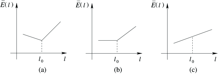
Figure 3: Schematic behaviour of the yrast spectrum in the vicinity of a plane-wave yrast state: (a) the inequalities in Eqs. (26) and (27) are satisfied and the yrast spectrum shows a cusp-like local minimum; (b) the inequalities are not satisfied but a slope discontinuity persists; (c) the plane-wave state is no longer an yrast state and the yrast spectrum is smooth through the angular momentum $l_{0}$.

To analyze the zeroes of $f(\Omega)$, we begin by assuming that the inequality in Eq. (27) is satisfied which implies $f(0)>0$. We now define the quartic $g(\Omega)\equiv f(\Omega)+4x_{A}x_{B}\gamma_{AB}^{2}$, which is simply $f(\Omega)$ shifted vertically by the constant $4x_{A}x_{B}\gamma_{AB}^{2}$. We also have $g(0)>0$. The solutions of $g(\Omega)=0$ are

$$(2\mu\pm\sqrt{2x_{A}\gamma_{AA}+1},\,\,2\nu\pm\sqrt{2x_{B}\gamma_{BB}+1}).$$ (53)

If the inequalities in Eqs. (26) and (27) are satisfied, two of these roots are negative and two are positive. Furthermore, $g^{\prime}(0)>0$, which implies that $g(\Omega)$ has a maximum at a point $\Omega>0$ between the largest negative root and the smallest positive root. By shifting $g(\Omega)$ down by $4x_{A}x_{B}\gamma_{AB}^{2}$ we recover $f(\Omega)$ and since $f(0)>0$, we conclude that $f(\Omega)=0$ must have four distinct, real roots, two of which are negative and two positive. These roots will be denoted by $\Omega_{1},...,\Omega_{4}$ with the ordering

$$\Omega_{1}<\Omega_{2}<0<\Omega_{3}<\Omega_{4}.$$ (54)

Recalling Eq. (47), these values are to be identified with the slope of the yrast spectrum at $l=l_{0}$. The fact that the energy at $l_{0}$ is a local minimum when the inequalities in Eqs. (26) and (27) are satisfied now implies that the left and right slopes of the yrast spectrum are necessarily $\Omega_{2}$ and $\Omega_{3}$, respectively. This establishes the fact that the slope of $\bar{E}_{0}(l)$ at $l_{0}$ is discontinuous if $\bar{E}[\psi_{A},\psi_{B}]$ has a local minimum at $(\phi_{\mu},\phi_{\nu})$. The qualitative behaviour of the yrast spectrum in the vicinity of $l_{0}$ is shown in Fig. 3(a).

Once the roots of Eq. (52) have been determined, Eq. (51) can be solved to yield

$$\frac{\delta c^{*}_{\mu+1}}{\delta c_{\mu-1}} =\frac{-2\mu+1+\Omega}{2\mu+1-\Omega};$$

$$\frac{\delta d_{\nu-1}}{\delta c_{\mu-1}} =\frac{(2\nu+1-\Omega)\left[(\Omega-2\mu)^{2}-2x_{A}\gamma_{AA}-1\right]}{2x_{B}\gamma_{AB}(2\mu+1-\Omega)};$$

$$\frac{\delta d^{*}_{\nu+1}}{\delta c_{\mu-1}} =-\frac{(2\nu-1-\Omega)\left[(\Omega-2\mu)^{2}-2x_{A}\gamma_{AA}-1\right]}{2x_{B}\gamma_{AB}(2\mu+1-\Omega)}.$$ (55)

Substituting the coefficients in Eq. (55) into Eq. (45) we find

$$\delta l=-\frac{|\delta c_{\mu-1}|^{2}}{x_{B}\gamma^{2}_{AB}(2\mu+1-\Omega)^{2}}\left\{4x_{A}x_{B}\gamma_{AB}^{2}(2\mu-\Omega)+(2\nu-\Omega)\left[(\Omega-2\mu)^{2}-2x_{A}\gamma_{AA}-1\right]^{2}\right\}.$$ (56)

Although it is difficult to see analytically, one can check numerically that $\delta l$ is indeed less than zero for $\Omega=\Omega_{2}$ and greater than zero for $\Omega_{3}$. This confirms that $\Omega_{2}$ and $\Omega_{3}$ correspond, respectively, to the portions of the yrast spectrum for $l<l_{0}$ and $l>l_{0}$.

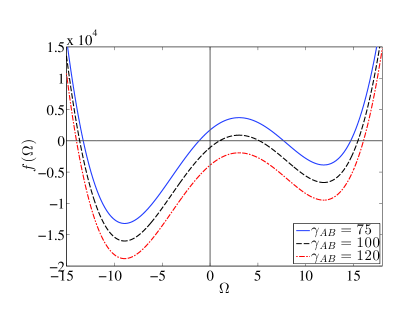
Figure 4: Evolution of the function $f(\Omega)$ with variations of $\gamma_{AB}$. Here $\mu=0$, $\nu=2$, $x_{B}=0.2$, $\gamma_{AA}=100$ and $\gamma_{BB}$ = 120. The critical $\gamma_{AB}$ for which the second root of $f(\Omega)$ becomes zero can be obtained from Eq. (52) and is found to be $\gamma_{AB}\simeq 91$. The critical $\gamma_{AB}$ for which the double root of $f(\Omega)$ emerges can be obtained from Eq. (57) and is found to be $\gamma_{AB}\simeq 107$.

We now suppose that a gradual variation of a system parameter leads to a violation of the inequality in Eq. (27). At this point, the state $(\phi_{\mu},\phi_{\nu})$ ceases to be a local minimum of the energy functional in Eq. (3). This evolution is easiest to visualize by considering variations in $\gamma_{AB}$ (see Fig. 4). As $\gamma_{AB}$ is increased, $f(\Omega)$ shifts down, with the effect that $\Omega_{2}$ increases and $\Omega_{3}$ decreases. Since $f^{\prime}(0)>0$, $\Omega_{2}$ will first go to zero at some critical value of $\gamma_{AB}$, at which point $\bar{E}_{0}(l)$ ceases to have a local minimum. This signals the fact that persistent currents are no longer stable at $l_{0}$. This is consistent with the criterion established earlier in Eqs. (26) and (27), since by setting $\Omega=0$ in Eq. (52) one recovers precisely the equality corresponding to Eq. (27). However, since $\Omega_{3}>0$ when $\Omega_{2}=0$, the derivative discontinuity in $\bar{E}_{0}(l)$ persists, as shown schematically in Fig. 3(b). As $\gamma_{AB}$ is increased further, the difference between the roots $\Omega_{2}$ and $\Omega_{3}$ gradually decreases and they eventually merge into a double root. At this point the discontinuity at $l_{0}$ vanishes, as indicated schematically in Fig. 3(c). In going from Fig. 3(b) to Fig. 3(c) we can envisage two possible scenarios. In the first, the plane-wave state is always an yrast state and the merging of the two roots establishes the critical condition for $(\phi_{\mu},\phi_{\nu})$ to be an yrast state. In other words, the plane-wave state at $l_{0}$ ceases to be an yrast state when the slope discontinuity vanishes. However, there is the possibility that a soliton state with an energy lower than that of the plane-wave state at $l_{0}$ may appear before the merging of the double root. If this happens, the emergence of the soliton state defines the critical condition for the plane-wave state to be an yrast state. In this case, the merging of the double root at best provides a bound on this critical condition. Whether or not this latter scenario actually occurs would have to be checked by explicit numerical solutions of the coupled Gross-Pitaevskii equations for the condensate wave functions.

In the following, we will assume that the first scenario discussed above is valid and therefore we will focus on the critical condition for which the quartic $f(\Omega)$ has a double root. This occurs when the discriminant $\Delta$ of the quartic is zero, that is

$$\Delta(x_{s},\gamma_{ss^{\prime}},\mu,\nu)\equiv{\rm det}(S)=0.$$ (57)

Here the discriminant is defined by the determinant of the so-called Sylvester matrix Gelfand

$$S=\left(\begin{array}[]{cccccccc}a_{4}&a_{3}&a_{2}&a_{1}&a_{0}&0&0\\ 0&a_{4}&a_{3}&a_{2}&a_{1}&a_{0}&0\\ 0&0&a_{4}&a_{3}&a_{2}&a_{1}&a_{0}\\ 4a_{4}&3a_{3}&2a_{2}&a_{1}&0&0&0\\ 0&4a_{4}&3a_{3}&2a_{2}&a_{1}&0&0\\ 0&0&4a_{4}&3a_{3}&2a_{2}&a_{1}&0\\ 0&0&0&4a_{4}&3a_{3}&2a_{2}&a_{1},\end{array}\right),$$ (58)

where $a_{4},...,a_{0}$ are the the coefficients of the quartic $f(\Omega)$ in Eq. (52), namely

$$a_{4} =1,$$

$$a_{3} =-4(\mu+\nu),$$

$$a_{2} =4(\mu^{2}+\nu^{2}+4\mu\nu)-2(x_{A}\gamma_{AA}+x_{B}\gamma_{BB}+1),$$

$$a_{1} =-4\nu(4\mu^{2}-2x_{A}\gamma_{AA}-1)-4\mu(4\nu^{2}-2x_{B}\gamma_{BB}-1),$$

$$a_{0} =(4\mu^{2}-2x_{A}\gamma_{AA}-1)(4\nu^{2}-2x_{B}\gamma_{BB}-1)-4x_{A}x_{B}\gamma_{AB}^{2}.$$ (59)

Alternatively, we can make use of the properties of $f(\Omega)$ to determine the critical condition for which the $\Omega_{2}$ and $\Omega_{3}$ roots merge and take the common value $\Omega_{0}$. We observe that $f^{\prime}(\Omega)$ is a cubic and that $f^{\prime}(\Omega)=0$ has three roots, as can be seen from Fig. 4. The frequency $\Omega_{0}$ is the root for which $f^{\prime\prime}(\Omega_{0})<0$. The condition $f^{\prime}(\Omega_{0})=0$ gives the equation

$$(\Omega_{0}-2\mu)\left[(\Omega_{0}-2\nu)^{2}-2x_{B}\gamma_{BB}-1\right]+(\Omega_{0}-2\nu)\left[(\Omega_{0}-2\mu)^{2}-2x_{A}\gamma_{AA}-1\right]=0.$$ (60)

Furthermore, we see that $f(\Omega_{0})=0$ when

$$\left[(\Omega_{0}-2\mu)^{2}-2x_{A}\gamma_{AA}-1\right]\left[(\Omega_{0}-2\nu)^{2}-2x_{B}\gamma_{BB}-1\right]=4x_{A}x_{B}\gamma_{AB}^{2}.$$ (61)

When Eqs. (60) and (61) are used in Eq. (56), we find that $\delta l$ becomes zero when $\Omega=\Omega_{0}$. Thus the merging of the $\Omega_{2}$ and $\Omega_{3}$ roots can be determined by requiring that $f(\Omega)=0$ and $\delta l=0$ be satisfied simultaneously. These two equations, a quartic and quintic respectively, have to be solved numerically and the critical condition found is identical to that obtained from Eq. (57).

Finally, we note that if the parameters $x_{s}$ and $\gamma_{ss^{\prime}}$ satisfy Eq. (57) they also satisfy the equations

$$\Delta(x_{s},\gamma_{ss^{\prime}},-\mu,-\nu)=0,$$ (62)

and

$$\Delta(x_{s},\gamma_{ss^{\prime}},\mu+n,\nu+n)=0,$$ (63)

where $n$ is an integer. This is due to the fact that the existence of a double root of $f(\Omega)$ is not affected by inversion of the function $f(\Omega)$ with respect to the $y$ axis or translation along the $x$ axis. As a result the critical condition can simply be written as

$$\Delta(x_{s},\gamma_{ss^{\prime}},0,|k|)=0,$$ (64)

where $k=\nu-\mu$. This agrees with the general observation we made at the beginning of this section that the condition for $(\phi_{\mu},\phi_{\nu})$ to be an yrast state should only depend on the absolute difference of $\mu$ and $\nu$. Furthermore, from Fig. 4 we see that the necessary condition for a slope discontinuity to occur in the yrast spectrum is that Eq. (52) has four real roots. The latter is ensured if the discriminant is positive, namely,

$$\Delta(x_{s},\gamma_{ss^{\prime}},0,|k|)>0.$$ (65)

Within the first scenario discussed earlier, the inequality in Eq. (65) constitutes the condition for $(\phi_{\mu},\phi_{\nu})$ being an yrast state.

III.2 Numerical results and discussion

In general, the discriminant $\Delta(x_{s},\gamma_{ss^{\prime}},|k|)$ is a rather complex function of $x_{B}$, $\gamma_{ss^{\prime}}$ and $k$ (we restrict ourselves to non-negative $k$ from now on). An exception occurs for $k=0$, where one finds that the inequality in Eq. (65) simplifies to

$$\left(2x_{A}\gamma_{AA}+1\right)\left(2x_{B}\gamma_{BB}+1\right)-4x_{A}x_{B}\gamma_{AB}^{2}>0.$$ (66)

This in fact coincides with the condition for stability of the ground state against phase separation (see Eq. (30)). As shown in Ref. Anoshkin , this stability condition follows from the requirement that the Bogoliubov excitations all have positive energies. The inequality in Eq. (66) thus ensures that the uniform state ($l=0$) is the ground state of the system and, by virtue of the periodicity of $e_{0}(l)$, the yrast states at all integral angular momenta are plane-wave states.

The case of $k\geq 1$, namely the condition for plane-wave yrast states at non-integer angular momentum, is of course more complex. However, in the $x_{B}\rightarrow 0$ limit, one finds that the condition in Eq. (65) reduces to

$$\gamma_{AA}>2k(k-1).$$ (67)

This suggests that $(\phi_{\mu},\phi_{\mu+k})$ is an yrast state if the interaction strength of the majority component satisfies Eq. (67) and the minority concentration is sufficiently small, regardless of the strength of $\gamma_{BB}$ and $\gamma_{AB}$. Similarly in the limit that $x_{B}\rightarrow 1$ the condition in Eq. (65) reduces to

$$\gamma_{BB}>2k(k-1).$$ (68)

To explore the consequences of interaction asymmetries on the emergence of certain plane-wave yrast states in more detail, we use the parameterization introduced earlier, namely, $\gamma_{AB}=\gamma$, $\gamma_{AA}=(1+\kappa_{A})\gamma$ and $\gamma_{BB}=(1+\kappa_{B})\gamma$. For each $k$, the critical condition

$$\Delta(x_{s},\gamma_{ss^{\prime}},0,|k|)\equiv\tilde{\Delta}(x_{B},\gamma,\kappa_{A},\kappa_{B},|k|)=0$$ (69)

then defines a hypersurface in the parameter space spanned by $x_{B}$, $\gamma$, $\kappa_{A}$ and $\kappa_{B}$. We will be primarily interested in the critical $x_{B}(\gamma,k)$ curves on such a hypersurface for fixed values of $\kappa_{A}$ and $\kappa_{B}$. We remind the reader that these critical curves are the analogue of the solid curves in Fig. 1 which define when certain plane wave states become yrast states in the symmetric model. These curves are recovered in the limit that $\kappa_{A}=\kappa_{B}=0$.

To be specific, we first consider the case of $\gamma_{AA}=\gamma_{BB}\neq\gamma_{AB}$, namely $\kappa_{A}=\kappa_{B}=\kappa\neq 0$. In Fig. 5 we show the critical $x_{B}(\gamma,k)$ curves, determined from Eq. (69), for $k=2$ and various values of $\kappa$. This figure shows how the limit of the symmetric model is approached as $\kappa$ tends to zero (the $k=2$ dashed curve in Fig. 1). Our first general observation is that these curves all possess a mirror symmetry with respect to the horizontal line $x_{B}=1/2$. This is due to the fact that for $\gamma_{AA}=\gamma_{BB}$, the discriminant $\Delta(x_{s},\gamma_{ss^{\prime}},\mu,\nu)$ in Eq. (57) is invariant under simultaneous interchanges between $x_{A}$ and $x_{B}$ and between $\mu$ and $\nu$. As a result, we have

$$\tilde{\Delta}(x_{B},\gamma,\kappa,\kappa,|k|)=\tilde{\Delta}(1-x_{B},\gamma,\kappa,\kappa,|k|),$$ (70)

which explains the mirror symmetry. We note that in generating Fig. 5, we are no longer restricting $x_{B}$ to be the minority concentration but are allowing it to vary continuously between 0 and 1. Presenting the results in this way more clearly displays the continuous variation of the $x_{B}(\gamma,k)$ curves. The range $0.5\leq x_{B}\leq 1$ of course corresponds to species $A$ being the minority concentration and provides no new information when $\gamma_{AA}=\gamma_{BB}$. However, when $\gamma_{AA}\neq\gamma_{BB}$, this form of the plots provides the relevant information more efficiently.

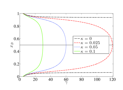
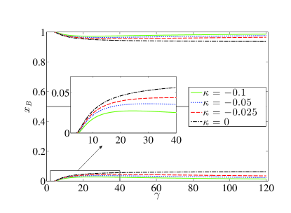
Figure 5: The plane-wave yrast state critical $x_{B}(\gamma,k)$ curves for $k=2$. Here $\kappa_{A}=\kappa_{B}=\kappa$ assume different values. The symmetric model is recovered in the $\kappa=0$ limit.

We next observe that the limiting $\kappa=0$ curve has a horizontal asymptote for $\gamma\to\infty$ Wu , which is approached from one side when $\kappa<0$ and from the other when $\kappa>0$. Thus the qualitative behaviour of the $x_{B}(\gamma,k)$ curves is quite different in these two cases. Although all the curves have an endpoint at $\gamma=2k(k-1)/(1+\kappa)$ (see Eqs. (67) and (68) for $\kappa_{A}=\kappa_{B}=\kappa$) only the curves for $\kappa>0$ (left panel in Fig. 5) cross the line $x_{B}=1/2$ perpendicularly at some critical $\gamma$ value. It can be shown from Eqs. (60) and (61) that this critical $\gamma$ value is given by the simple formula

$$\gamma_{\rm cr}=\frac{k^{2}-1}{\kappa}.$$ (71)

If a point in the $\gamma$-$x_{B}$ plane lies to the right of the $x_{B}(\gamma,k)$ curve, then $(\phi_{\mu},\phi_{\mu+k})$ is an yrast state for the given values of the system parameters. For the example being considered in Fig. 5, the point (40, 0.3) lies to the right of the $x_{B}(\gamma,2)$ curve for $\kappa=0.1$ but to the left of the curve for $\kappa=0.05$. This implies that the $(\phi_{0},\phi_{2})$ plane-wave state ceases to be an yrast state at $x_{B}=0.3$ as $\kappa$ is decreased continuously from 0.1 to 0.05. This behaviour is consistent with the discussion given in the Appendix. The value of $\delta\bar{E}_{\rm int}$ given in Eq. (78) decreases with decreasing $\kappa$ so that the conditions required for the $(\phi_{0},\phi_{2})$ plane-wave state to be an yrast state are eventually violated. The main conclusion we reach for this kind of asymmetry is that larger positive values of $\kappa$ favour a plane-wave state being an yrast state.

For $\kappa<0$ on the other hand (right panel in Fig. 5), the curves are bounded by the $\kappa=0$ curves and the $x_{B}=0$ or $x_{B}=1$ lines and tend to these lines in the large $\gamma$ limit. We see that the region in the $\gamma$-$x_{B}$ plane where the plane-wave state is an yrast state diminishes in size as $\kappa$ is made more negative. Thus negative $\kappa$ disfavours a plane-wave state being an yrast state. It is clear that the conditions for a plane-wave state being an yrast state are very sensitive to the sign of $\kappa$ and that the case of symmetric interactions ($\kappa=0$) is a very special one. The inset to the right panel of Fig. 5 shows more clearly how the $x_{B}(\gamma,k)$ curves approach the $x_{B}=0$ line as $\gamma\to\infty$. We have here a situation in which at some $x_{B}$ value, a plane-wave state can become an yrast state with increasing $\gamma$ but then ceases to be an yrast state with further increases in $\gamma$.

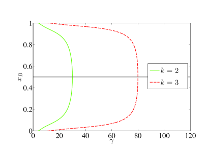
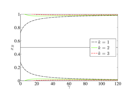
Figure 6: The plane-wave yrast state critical $x_{B}(\gamma,k)$ curves for $k=1,2,3$, with $\kappa=0.1$ (left panel) and $\kappa=-0.1$ (right panel). As explained in the text, the plane wave states $(\phi_{\mu},\phi_{\mu+1})$ are yrast states for any $x_{B}$ when $\kappa>0$, which explains the absence of the $k=1$ critical curve in the left panel.

In Fig. 6 we show the $x_{B}(\gamma,k)$ curves for different $k$, again for the case $\gamma_{AA}=\gamma_{BB}$. The left panel is for $\kappa=0.1$ and the right for $\kappa=-0.1$. For the symmetric model it is known that the $(\phi_{0},\phi_{1})$ state is an yrast state for all $x_{B}$ and any positive value of $\gamma$. As explained in the Appendix, this state is necessarily also an yrast state when $\kappa>0$, and for this reason, there is no critical curve for $k=1$ in this case. For both signs of $\kappa$ we see that the conditions for a plane-wave state being an yrast state become more stringent with increasing $k$. The curves are qualitatively similar to those in Fig. 5 except for the $k=1$ curve with $\kappa<0$. In this case, the endpoint of the $x_{B}(\gamma,1)$ curve is a point on the $x_{B}$-axis. As $\kappa\to 0^{-}$, the $x_{B}(\gamma,1)$ curves approach $x_{B}=1/2$ and the $k=1$ state is an yrast state for all $x_{B}$ and $\gamma$. This implies that the region in the $x_{B}$-$\gamma$ plane between the $k=1$ critical curves is the region where the $k=1$ state is not an yrast state.

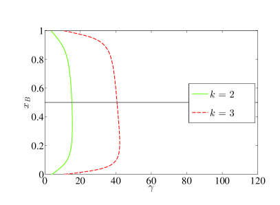
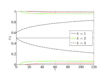
Figure 7: The plane-wave yrast state critical $x_{B}(\gamma,k)$ curves for $k=1,2,3$, where $\kappa_{A}=0.1$ and $\kappa_{B}=0.3$ in the left panel, and $\kappa_{A}=0.1$ and $\kappa_{B}=-0.1$ in the right panel. The $x_{B}(\gamma,1)$ curve is once again absent in the left panel since the $k=1$ plane-wave state is an yrast state for all $x_{B}$ when $\kappa_{A}>0$ and $\kappa_{B}>0$.

Finally we show in Fig. 7 some examples of critical $x_{B}(\gamma,k)$ curves for the system with the most general type of interaction asymmetry $\kappa_{A}\neq\kappa_{B}\neq 0$. We find that these curves are qualitatively similar to those for $\kappa_{A}=\kappa_{B}\neq 0$, with one obvious difference, namely the absence of mirror symmetry with respect to $x_{B}=1/2$ line. For $0\leq x_{B}\leq 0.5$, $B$ is the minority species and $\kappa_{B}$ is the minority asymmetry parameter. On the other hand, for $0.5\leq x_{B}\leq 1$, $A$ is the minority species and $\kappa_{A}$ is the minority asymmetry parameter. These figures can thus be viewed as providing the critical curves for two different sets of asymmetry parameters for the minority and majority species.

The curves for $k=1$ in the right panel of Fig. 7 show an interesting asymmetry. The $k=1$ critical curve in the range $0\leq x_{B}\leq 0.5$ has an endpoint at $x_{B}=1/2$ at $\gamma=0$. This is true whenever the minority asymmetry parameter $\kappa_{B}$ is less than zero. As $\kappa_{B}\to 0^{-}$, this curve moves continuously to the $x_{B}=1/2$ line. However, when the minority species is $A$ with $\kappa_{A}>0$, the critical curve has an endpoint on the $x_{B}$ axis that depends on the value of $\kappa_{A}$. As $\kappa_{A}\to 0^{+}$, this point moves to $x_{B}=0.5$ and the whole critical curve approaches the $x_{B}=1/2$ line.

IV Concluding remarks

In this paper we have studied the structure of the mean-field yrast spectrum of a two-component gas in the ring geometry with arbitrary inter-particle interaction strengths. In the case of the symmetric model, the nature of the spectrum can be elucidated by means of analytic soliton solutions of the coupled GP equations Smyrnakis2 ; Wu . Such solutions, however, are not known for the asymmetric model in which the interaction strengths take on different values. Nevertheless, we were able to show that some of the salient properties of the yrast spectrum can be determined via a perturbative analysis of the GP energy functional. In particular, we derived criteria, expressed in terms of inequalities, which determine whether a specific plane-wave state is a local minimum of the GP energy functional. We then assumed that the global minimum of the energy functional on the angular momentum hypersurface corresponding to this plane-wave necessarily occurs at that particular plane-wave state. Furthermore, if the GP energy functional has a local minimum at this state, the yrast spectrum does as well and persistent currents are thus stable Bloch at the angular momentum of the plane-wave state. We then showed that the yrast spectrum at these angular momenta has slope discontinuities which persist even after the yrast spectrum ceases to exhibit a local minimum. Finally, we showed that the plane-wave state ceases to be an yrast state when the system parameters satisfy a certain critical condition.

In the future we plan a more detailed numerical investigation of the yrast spectrum based on the solution of the coupled GP equations for the condensate wave functions. Such a study would provide the solitonic portions of the yrast spectrum that join the plane-wave yrast states that we have analysed in this paper.

Appendix A

In this Appendix, we investigate the yrast spectrum in the angular moment interval $0\leq l\leq 1/2$. As discussed in Sec. II, the plane-wave states of interest in this angular momentum range are $(\phi_{\mu},\phi_{\mu+k})$ with angular momentum $l=\mu+kx_{B}$, where $k$ is an integer restricted to the range given by Eq. (12). We argue that such a state can indeed be an yrast state if the intra-species interaction strengths $\gamma_{AA}$ and $\gamma_{BB}$ are both sufficiently large in comparison to the inter-species interaction strength $\gamma_{AB}$. In effect we are claiming that conditions exist for which the state $(\mu,\mu+k)$ is assured to be a global minimum on the $l=\mu+kx_{B}$ hypersurface. We emphasize, however, that in general these are sufficient but not necessary conditions. As found previously, it is possible for these plane-wave states to be yrast states even in the symmetric model where all the interaction parameters are the same.

Our objective is to determine whether the plane-wave state $(\mu,\mu+k)$ can be a global minimum of the GP energy functional on the $l=\mu+kx_{B}$ hypersurface. To investigate this possibility we consider the wave functions

$$\psi_{A}=\phi_{\mu}+\delta\psi_{A},\quad\psi_{B}=\phi_{\nu}+\delta\psi_{B},$$ (72)

where $\nu=\mu+k$ and

$$\delta\psi_{A}=\sum_{m}\delta c_{m}\phi_{m},\quad\delta\psi_{B}=\sum_{m}\delta d_{m}\phi_{m}.$$ (73)

Here, the deviations $\delta c_{m}$ and $\delta d_{m}$ are not necessarily small, and for certain choices, can in fact lead to another pair of plane waves. However, as established in Sec. II, the state $(\phi_{\mu},\phi_{\nu})$ has the lowest energy of all the plane wave states with the same angular momentum.

The difference in energy between the $(\psi_{A},\psi_{B})$ and $(\phi_{\mu},\phi_{\nu})$ states can be written as

$$\delta\bar{E}=\delta\bar{E}_{K}+\delta\bar{E}_{\rm int}.$$ (74)

Here

$$\delta\bar{E}_{K}=x_{A}\sum_{m}m^{2}|\delta c_{m}|^{2}+x_{B}\sum_{m}m^{2}|\delta d_{m}|^{2}+x_{A}\mu^{2}\left(\delta c_{\mu}+\delta c_{\mu}^{*}\right)+x_{B}\nu^{2}\left(\delta d_{\nu}+\delta d_{\nu}^{*}\right)$$ (75)

and

$$\delta\bar{E}_{\rm int}=x_{A}^{2}\pi\gamma_{AA}\int_{0}^{2\pi}d\theta\left|\delta\rho_{A}(\theta)\right|^{2}+x_{B}^{2}\pi\gamma_{BB}\int_{0}^{2\pi}d\theta\left|\delta\rho_{B}(\theta)\right|^{2}+2x_{A}x_{B}\pi\gamma_{AB}\int_{0}^{2\pi}d\theta\delta\rho_{A}(\theta)\delta\rho_{B}(\theta),$$ (76)

where $\delta\rho_{s}=|\psi_{s}|^{2}-|\phi_{s}|^{2}$. We note that the change in interaction energy $\delta\bar{E}_{\rm int}$ is zero whenever $(\psi_{A},\psi_{B})$ is a plane-wave state.

We now consider the difference in kinetic energy $\delta\bar{E}_{\rm K}$ in more detail. Using the normalization constraints (18) and (19) in Eq. (75) we find

$$\delta\bar{E}_{K}=x_{A}\sum_{m}(m^{2}-\mu^{2})|\delta c_{m}|^{2}+x_{B}\sum_{m}(m^{2}-\nu^{2})|\delta d_{m}|^{2}$$ (77)

It is apparent that the change in kinetic energy $\delta\bar{E}_{K}$ can be made negative with appropriate wave function variations. The argument we make depends simply on the fact that $\delta\bar{E}_{K}$ has a lower bound $\delta\bar{E}_{l.b.}$. The kinetic energy of the plane-wave state $(\phi_{\mu},\phi_{\nu})$ is $\bar{E}_{K}[\phi_{\mu},\phi_{\nu}]=x_{A}\mu^{2}+x_{B}\nu^{2}$. Since the kinetic energy functional $\bar{E}_{K}[\psi_{A},\psi_{B}]$ is positive semi-definite, the lowest possible value it can have is 0. Thus the lower bound is given by $\delta\bar{E}_{l.b.}=-(x_{A}\mu^{2}+x_{B}\nu^{2})$. It should be noted that this lower bound is reached only for the $(\phi_{0},\phi_{0})$ state which does not lie on the angular momentum hypersurface of interest. Nevertheless, this lower bound must still be valid when variations of the wave functions are constrained to have the desired angular momentum.

The interaction energy in Eq. (76) can be written as

$$\delta\bar{E}_{\rm int}=x_{A}^{2}\pi(\gamma_{AA}-\gamma_{AB})\int_{0}^{2\pi}d\theta\left|\delta\rho_{A}(\theta)\right|^{2}+x_{B}^{2}\pi(\gamma_{BB}-\gamma_{AB})\int_{0}^{2\pi}d\theta\left|\delta\rho_{B}(\theta)\right|^{2}+\pi\gamma_{AB}\int_{0}^{2\pi}d\theta|\delta\rho(\theta)|^{2},$$ (78)

where $\delta\rho=x_{A}\delta\rho_{A}+x_{B}\delta\rho_{B}$ is the total change in particle density. Eq. (78) reduces to the change in interaction energy in the symmetric model with $\gamma=\gamma_{AB}$ when $\gamma_{AA}=\gamma_{BB}=\gamma_{AB}$. If the $(\mu,\nu)$ plane-wave state is an yrast state in the symmetric model for this value of $x_{B}$ and interaction parameter $\gamma$, then this state remains an yrast state in the asymmetric model with $\gamma_{AA}>\gamma_{AB}$ and $\gamma_{BB}>\gamma_{AB}$ since the interaction energy only increases while the change in kinetic energy is unaltered. If this state is not an yrast state in the symmetric model it is still possible that it becomes an yrast state in the asymmetric model. We now turn to the demonstration of this possibility.

Equation (78) implies

$$\delta\bar{E}_{\rm int}\geq x_{A}^{2}\pi(\gamma_{AA}-\gamma_{AB})\int_{0}^{2\pi}d\theta\left|\delta\rho_{A}(\theta)\right|^{2}+x_{B}^{2}\pi(\gamma_{BB}-\gamma_{AB})\int_{0}^{2\pi}d\theta\left|\delta\rho_{B}(\theta)\right|^{2}.$$ (79)

which is positive-definite if both $\gamma_{AA}$ and $\gamma_{BB}$ are greater than $\gamma_{AB}$. Since $\delta\bar{E}_{K}$ can be negative, the question of interest is whether $\delta\bar{E}$ can be made positive-definite with a suitable choice of parameters. Specifically, we wish to determine whether conditions exist such that

$$\delta\bar{E}_{\rm int}>|\delta\bar{E}_{K}|$$ (80)

for any wave function having the same angular momentum but with a lower kinetic energy, i.e. $\delta\bar{E}_{K}<0$.

Figure 8: The schematic variation of $\delta\bar{E}_{\rm int}$ and $\delta\bar{E}_{K}$ along a path on the angular momentum hypersurface between the kinetic energy minimizing plane-wave state at 1 and some other plane-wave state at 2. $\delta\bar{E}_{\rm int}$ increases in magnitude as $\gamma_{AA}$ and $\gamma_{BB}$ are increased relative to $\gamma_{AB}$. It is assumed that $\delta\bar{E}_{K}$ becomes negative along parts of the path; the dashed curve indicates the lower bound on $\delta\bar{E}_{K}$.

In Fig. 8 we illustrate the expected qualitative variation of $\delta\bar{E}_{\rm int}$ and $\delta\bar{E}_{K}$ along some path on the angular momentum hypersurface between the plane-wave state minimizing the kinetic energy and some other plane-wave state that has a higher kinetic energy. Along this path $\delta\bar{E}_{\rm int}$ is positive and vanishes at the ends of the path. The dashed line indicates the lower bound on $\delta\bar{E}_{K}$. Since $\delta\bar{E}_{\rm int}$ can be made arbitrarily large by increasing $\gamma_{AA}$ and $\gamma_{BB}$ relative to $\gamma_{AB}$, it is clear that $\delta\bar{E}_{\rm int}$ can be made to satisfy the inequality in Eq. (80) except possibly at the start of the path at 1 where it goes to zero. However, at this point we know that, if Eqs. (26) and (27) are satisfied, $\bar{E}$ has a local minimum at this point. Thus, even if $\delta\bar{E}_{K}$ were to decrease as one moved away from 1, the local minimum at this point would ensure that Eq. (80) is satisfied. Since the inequalities in Eqs. (26) and (27) become even stronger with increasing $\gamma_{AA}$ and $\gamma_{BB}$, it is clear that it is always possible to ensure that Eq. (80) is satisfied at all points along the path from 1 to 2 where $\delta\bar{E}_{K}$ is negative. This observation implies that the plane-wave state at 1 can be made a global minimum on the angular momentum hypersurface for a suitable choice of the interaction parameters. In the body of the paper we make the stronger assumption that the plane-wave state is a global minimum when the inequalities in Eqs. (26) and (27) are satisfied. All our results are consistent with this assumption.

References

- (1) S. Gupta, K. W. Murch, K. L. Moore, T. P. Purdy, and D. M. Stamper-Kurn, Phys. Rev. Lett. 95, 143201 (2005).
- (2) C. Ryu, M. F. Andersen, P. Cladé. V. Natarajan, K. Helmerson, and W. D. Phillips, Phys. Rev. Lett. 99, 260401 (2007).
- (3) B. E. Sherlock, M. Gildemeister, E. Owen, E. Nugent, and C. J. Foot, Phys. Rev. A 83, 043408 (2011).
- (4) A.Ramanatha, K. C. Wright, S. R. Muniz, M. Zelan, W. T. Hill III, C. J. Lobb, K. Helrmerson, W. D. Phillips, and G. K. Campbell, Phys. Rev. Lett. 106, 130401 (2011).
- (5) S. Moulder, S. Beattie, R. P. Smith, N. Tammuz, and Z. Hadzibabic, Phys. Rev. A 86, 013629 (2012).
- (6) S. Beattie, S. Moulder, R. J. Fletcher, and Z. Hadzibabic, Phys. Rev. Lett. 110, 025301 (2013).
- (7) J. R. Anglin, Phys. Rev. Lett. 87, 240401 (2001).
- (8) R. Dubessy, T. Liennard, P. Pedri, and H. Perrin, Phys. Rev. A 86, 011602 (2012).
- (9) A. I. Yakimenko, K. O. Isaieva, S. I. Vilchinskii, and M. Weyrauch, Phys. Rev. A 88, 051602 (2013).
- (10) M. Abad, A. Santori, S. Finazzi, and A. Recati, Phys. Rev. A 89, 053602 (2014).
- (11) A. I. Yakimenko, Y. M. Bidasyuk, M. Weyrauch, Y. I. Kuriatnikov, and S. I. Vilchinskii, Phys. Rev. A 91, 033607 (2015).
- (12) F. Bloch, Rhys. Rev. A 7, 2187 (1973).
- (13) The yrast terminology was introduced into cold-atom physics in B. Mottelson, Phys. Rev. Lett. 83 2695 (1999).
- (14) J. Smyrnakis, S. Bargi, G. M. Kavoulakis, M. Magiropoulos, K. Karkkainen, and S. M. Reimann, Phys. Rev. Lett. 103, 100404 (2009).
- (15) K. Anoshkin, Z. Wu, and E. Zaremba, Phys. Rev. A 88, 013609 (2013).
- (16) J. Smyrnakis, M. Magiropoulos, G. M. Kavoulakis and A. D. Jackson, Phys. Rev. A 87, 013603 (2013).
- (17) J. Smyrnakis, M. Magiropoulos, A. D. Jackson, and G. M. Kavoulakis, J. Phys. B 45, 235302 (2012).
- (18) Z. Wu and E. Zaremba, Phys. Rev. A 88, 063640 (2013).
- (19) J. Smyrnakis, M. Magiropoulos, N. K. Efremidis and G. M. Kavoulakis, J. Phys. B: At. Mol. Opt. Phys. 4, 215302 (2014).
- (20) I. M. Gelfand, M. M. Kapranov and A. V. Zelevinsky, Discriminants, resultants and multidimensional determinants (Birkhuser, Boston, 1994).