GRASIL-3D: an Implemention of Dust Effects in the SEDs of Simulated Galaxies

Abstract

We introduce a new model for the spectral energy distribution of galaxies, GRASIL-3D, which includes a careful modelling of the dust component of the interstellar medium. GRASIL-3D is an entirely new model based on the formalism of an existing and widely applied spectrophotometric model, GRASIL, but specifically designed to be interfaced with galaxies with any arbitrarily given geometry, such as galaxies calculated by theoretical hydrodynamical galaxy formation codes. GRASIL-3D is designed to separately treat radiative transfer in molecular clouds and in the diffuse cirrus component. The code has a general applicability to the outputs of simulated galaxies, either from Lagrangian or Eulerian hydrodynamic codes. As an application, the new model has been interfaced to the P-DEVA and GASOLINE smoothed-particle hydrodynamic codes, and has been used to calculate the spectral energy distribution for a variety of simulated galaxies from UV to sub-millimeter wavelengths, whose comparison with observational data gives encouraging results. In addition, GRASIL-3D allows 2D images of such galaxies to be obtained, at several angles and in different bands.

1 INTRODUCTION

The investigation of the process of galaxy formation and evolution by means of hydrodynamical simulations, though not yet producing a well defined and unique picture (see for instance Scannapieco et al., 2012), has nevertheless already provided fundamental insights. A basic limitation is that most of the processes driving the evolution of luminous matter, which has also some back-reaction on dark matter (DM), occurs many orders of magnitude below the resolution of any feasible cosmological simulation, and are also poorly understood. They are implemented in the simulation by means of approximate and uncertain prescriptions, containing several adjustable parameters. In any case, when compared to the alternative approach followed in the literature to understand the origin of galaxy populations, namely the so called Semi Analytic Models (SAMs), simulations provide, at least in principle, information on the 6D phase space as a function of time, i.e. a detailed dynamical information. They also provide, for each particle or volume element depending on the implementation, ages of the stellar component and temperature of the gaseous one, and, when metal enrichment is implemented, chemical composition of both.

However, to compare this rich information with the huge data sets available nowadays, the quite delicate and complex step of predicting the multi-wavelength Spectral Energy Distributions (SED) of mock objects is required. Indeed, while simulations by themselves only trace the evolution of mass, observations trace light. The huge amount of multi-wavelength data collected in the last decades have evidenced a fundamental complication and uncertainty of this step, namely the significant reprocessing of light emitted by primary sources (stars or active galactic nuclei) by means of the dusty Inter Stellar Medium (ISM). Due to this effect, which tends to be increasingly important in galaxies characterized by higher specific star formation rates, the predicted SED has a strong dependence on the relative geometry of stars and dust, as well as on the optical properties of dust grains. Both on theoretical as well as on empirical ground the latter are expected to vary from galaxy to galaxy, and are difficult to predict (e.g. Calura et al., 2008; Schurer et al., 2009; Rocca-Volmerange et al., 2013).

Therefore to test the simulations against observations, it is essential to interface their outputs with tools that can predict a multi-wavelength SED, including a careful treatment of the radiation transfer through the dust. A few tools already exist for this purpose, for example: SUNRISE (Jonsson, 2004, 2006; Jonsson et al., 2010); RADISHE (Chakrabarti et al., 2008; Chakrabarti & Whitney, 2009); Art2 (Li et al., 2007, 2008; Yajima et al., 2012), all using Monte Carlo techniques to follow the radiation of photons through the diffuse ISM and to calculate a global radiation field, and hence the dust re-emission. In addition SUNRISE includes the treatment of star-forming regions using the dust and photo-ionization code MAPPINGSIII (Groves et al., 2008).

RADISHE is a self-consistent three-dimensional code to solve radiative transfer under the assumption of radiative equilibrium, using a Monte Carlo code based on the Lucy (1999) algorithm. Dust is assumed to be in thermal equilibrium with the radiation field, and the energy it absorbs is re-emitted as thermal emission. Therefore, the effects of the stochastically heated small grains on the SEDs are not considered.

ART² also uses a Monte Carlo technique to solve the radiative transfer in dusty media under the assumption of radiative equilibrium, adding two modules that couple the continuum and Ly$\alpha$ line emissions, and take into account the effects of ionization and dust absorption in the propagation and scattering of photons. The Continuum module of ART² was developed by Li et al. (2008), who adopted the radiative equilibrium algorithm by Bjorkman & Wood (2001). The new ART² version includes the treatment of Ly$\alpha$ radiative transfer in dusty and ionized ISM as its particular improvements.

In a somewhat different context, the dust radiative-transfer model GRASIL (Silva et al., 1998; Silva, 1999, hereafter S98 and S99 respectively) has been used highly successfully for many years, in two main ways: i), In combination with a simple chemical evolution model, CHE$\_$EVO, in order to calculate SEDs, which have then been used to study individual galaxies, inferring galaxies properties such as star-formation histories and dust masses (e.g. Panuzzo et al., 2007; Calura et al., 2008; Iglesias-Páramo et al., 2007; Vega et al., 2008; Lo Faro et al., 2013), and ii), in combination with more sophisticated galaxy evolution models, particularly SAMs of galaxy formation (e.g. Granato et al., 2000, 2004; Baugh et al., 2005; Lacey et al., 2008; Cook et al., 2009; Fontanot et al., 2009; Silva et al., 2012), in order to predict SEDs which can be compared to observed ones, thereby testing the proposed galaxy formation scenarios. The GRASIL code has been used successfully with the GALFORM model (Cole et al., 2000; Granato et al., 2000; Baugh et al., 2005; Lacey et al., 2008), the MORGANA model (Monaco et al., 2007; Fontanot et al., 2008, 2009); and the ABC model (Granato et al., 2004; Silva et al., 2005; Lapi et al., 2006; Cook et al., 2009). It has been the first model to take into account the age-dependent dust reprocessing of stellar populations, arising from the fact that younger stars are associated with denser ISM environments. GRASIL can use the outputs from SAMs, in particular star formation and chemical enrichment histories, as well as the limited geometric information they provide, in order to produce self-consistent SEDs of mock galaxies relatively quickly. Moreover, a substantially faster version of the code was presented recently (Silva et al., 2011, 2012), exploiting artificial neural networks, which leads to improved usability in this area. However, despite the many strengths, it assumes equatorial and axial symmetry for the galaxy. While this is highly suitable for SAMs, which do not calculate a more detailed spatial distribution of stars and gas explicitly, the use of GRASIL in coupling with galaxies produced by hydro-simulations would imply the loss of a large quantity of useful information.

This paper presents a new model, GRASIL-3D, based on the GRASIL formulism, but designed to be applied to any hydrodynamic simulation. The motivation for this work comes from adapting in our new code the main concepts of an established code, GRASIL, which has already proved so successful in describing galaxies of many different types, thereby building on its strengths.

GRASIL solves the radiative-transfer equation under the condition of thermal equilibrium for dust grains bigger than a given size $a\geq a_{flu}$ (usually taken to be 250 Å), with a size-dependent temperature. However, for smaller grains a single gray body spectrum has been found not to work correctly. Indeed, as first noted by Greenberg (1968), small grains can be stochastically heated to temperatures much higher than the temperature that they would be expected to reach if they were in temperature equilibrium. Thus a more detailed calculation for smaller grains is required, as in the Guhathakurta & Draine (1989) method incorporated in GRASIL. This allows a proper treatment of small grains and of polycyclic aromatic hydrocarbons (PAHs) features dominating the mid-infrared (MIR) in some cases.

The paper is organized as follows: in $\S$2 we describe the GRASIL-3D model and how we interface it with the outputs from hydro codes. Tests of the new code are presented in $\S$3, and in $\S$4 some applications to calculate the SEDs, flux density ratios, colors and images of simulated galaxies at different stages of evolution are discussed. In $\S$5 the effects of model parameter variations within their allowed ranges are analyzed and discussed. Finally, in $\S$6 we summarize and discuss the main results of this paper and present its main conclusions.

2 Calculating the SEDs of Simulated Galaxies

To develop the GRASIL-3D code, we have followed the main characteristics and scheme of GRASIL, which we briefly recall here. The gas is subdivided in a dense phase (fraction $f_{mc}$ of the total mass of gas) associated with young stars (star-forming molecular clouds, MCs) and a diffuse phase (cirrus) where more evolved (free) stars and MCs are placed. The young stars leave the parent clouds in the time-scale $t_{0}$. The MCs are represented as spherical clouds with optical depth $\tau\propto\delta\,m_{mc}/r_{mc}^{2}$ (where $\delta$ is the dust to gas mass ratio, $m_{mc}$ is the mass of MCs, and $r_{mc}$ is their radius), with a central source, whose radiative transfer trough the MCs is computed. The radiative transfer of the radiation emerging from MCs and that from free stars is then computed through the cirrus dust (for more details see S98 and S99).

The aim of GRASIL-3D is to calculate multi-wavelength SEDs and images of simulated galaxies identified in simulations run with either Lagrangian or Eulerian codes. We recall that the former follow the evolution of particles, while the latter describe the relevant dynamical evolution through functions of position and time. In the case of Lagrangian codes, the particles are classified into dark, gaseous or stellar. Each galaxy-like-object produced in the simulations is sampled by particles of these three kinds. However, dark matter plays no role in the determination of the galaxy SEDs.

The main quantities that determine the SED are the star formation history, the mass of gas and the metallicity of stars and gas. In simple models these quantities are relatively simple functions of time, and the information on their spatial distributions, if present, is limited to the scale radii of stars and gas for an analytical and symmetrical density profile. In the case of simulated galaxies from hydro-codes, the outputs provide detailed information on the spatial distribution of stars, gas, possibly of their metallicity, in addition to the age distribution of stars. All these quantities are then output at different snapshots.

2.1 Simulation Code Outputs

Smoothing procedures on direct outputs, or direct outputs themselves in the case of Eulerian codes, provide, among other functions, the following spatial mass distributions necessary for the SEDs:

1. Stellar matter distribution, $\rho_{x*}(\vec{r},t)$, $x$ here specifies particular properties of the stellar populations, for example $x$ = $y$ (young) or $f$ (free).

2. Gaseous matter distribution, $\rho_{x}(\vec{r},t)$, $x$ here specifies particular properties of the gas particles (e.g. ”mc” for the dense phase, or ”c” for the cirrus)

3. Codes where metal enrichment is implemented, provide the stellar or gaseous metallicity $Z_{x}(\vec{r},t)$, where again $x$ specifies particular properties of the gaseous or stellar particles, for example, ”cold gas” or ”young stellar population”.

In this paper we focus on how to work with the outputs of Lagragian codes using particles, the adaptations needed to work with Eulerian codes being straighforward.

To smooth out the functions above, GRASIL-3D uses a cartesian grid whose cell size is set by the smoothing length used in the simulation code. The smoothed functions provide the geometry of the different simulated galaxy components, their position dependence $\vec{r}$ indicating that they are expected to miss any symmetry.

Given these outputs, we need to specify in detail how to implement in GRASIL-3D the space distributions $\rho_{mc}(\vec{r},t)$ (see $\S$2.2), and $\rho_{c}(\vec{r},t)$ for the diffuse ISM (see $\S$2.3), including a dust model and a scheme for the radiative transfer within these two components (see $\S$2.5.1 and $\S$2.5.2).

2.2 Implementation of the Space Distribution of the MC Component

For the star forming molecular clouds, we follow the main characteristics of their modeling in GRASIL, but taking advantage of the new possibilities provided by the detailed outputs of the simulations. In GRASIL the mass in the MC component in a given object at time $t_{G}$, $M_{mc}$, is set by the parameter $f_{mc}=M_{mc}/M_{gas}$, where $M_{gas}$ is the model gas mass at $t_{G}$. This is a free global parameter.

Here we derive $f_{mc}$ under the assumption that MCs are defined by a threshold, $\rho_{mc,thres}$, and by a probability distribution function (PDF) in the gas density pattern the simulation returns (see below). With these quantities, we get the total amount $M_{mc}$ of gas in the dense phase, and correspondingly the amount and density field of the diffuse gas. In principle, also the density field for the dense phase of the ISM could be defined in this way, but here we make the assumption that all the MCs are active, i.e., they are associated with star formation, as in GRASIL. Therefore, after defining $M_{mc}$, we distribute it following $\rho_{y*}(\vec{r},t)$ (the density of young stars, see 2.2.6). This prescription is in a sense equivalent to smoothing out the subresolution MC field, given by the PDF, to the scale of the young stellar field, that is, to the scale of the simulation resolution, see below. In this way, the free and young stellar field, as well as the MC field, are resolved as given by the simulation, while the diffuse gaseous field (cirrus) is described at subresolution scales by the PDF .

2.2.1 The probability distribution function

The PDF is a model for the gas distribution at sub-resolution scales characterized by two parameters $\rho_{0}$ and $\sigma$.

Simulations at $\sim 1$ kpc scales indicate that either $f_{pd}(\rho)d\rho$ (i.e., the number of cells with densities in the range $[\rho,\rho+d\rho]$) or $f_{pd,M}(\rho)d\rho$ (i.e., the mass fraction in cells whose density is in the range $[\rho,\rho+d\rho]$) can be fit by log-normal functions, characterized by a dispersion $\sigma$ (the same for both of them) and a density parameter, $\rho_{0}$ and $\rho_{0,M}=\rho_{0}e^{\sigma^{2}}$, respectively. The expression for $f_{pd}(\rho)d\rho$ is:

$$f_{pd}(\rho)d\rho=\frac{1}{\sqrt{2\pi}\sigma}\exp[-\frac{\ln(\rho/\rho_{0})^{2}}{2\sigma^{2}}]d\ln\rho$$ (1)

The volume-averaged density $<\rho>_{V}$, and mass-averaged density $<\rho>_{M}$ are given, respectively, by (see, for example, Elmegreen, 2002, and Wada & Norman 2007):

$$<\rho>_{V}=\rho_{0}e^{\sigma^{2}/2};<\rho>_{M}=\rho_{0}e^{2\sigma^{2}}$$ (2)

providing a relationship between the $\rho_{0}$ and $\sigma$ parameters.

2.2.2 Calculating $M_{mc}$

The fraction of gas in molecular clouds $f_{mc}(\vec{r},t)$ can be calculated from a theoretical PDF, assuming that cold gas with density $>\rho_{mc,thres}$ is in the form of MCs. More specifically, the calculation of $f_{mc}(\vec{r},t)$ has been made as follows:

1. Choose a PDF for the cold gas, $f_{pd}(ln\rho;ln\rho_{0};\sigma)$, see Section 2.2.1.

2. Choose a density threshold for MC formation $\rho_{mc,thres}$.

3. To determine the fraction of MC mass in the $i$-th particle at position $\vec{r}_{i}$ relative to cold gas, we calculate:

   $$f_{mc}(\vec{r}_{i};\rho_{mc,thres},\rho_{0},\sigma)=\frac{I(\rho_{mc,thres},\rho_{0},\sigma))}{I(0;\rho_{0},\sigma)}$$ (3)

   where

   $$I(\rho_{min},\rho_{0},\sigma)=\int_{\ln\rho_{min}}^{\infty}\rho f_{pd}(\ln\rho;\ln\rho_{0};\sigma)d\ln\rho$$ (4)

   That is (Wada & Norman, 2007, Eq. 18 and 19):

   $$f_{mc}(\vec{r}_{i};\rho_{mc,thres},\rho_{0},\sigma)=0.5(1-Erf[z(\rho_{mc,thres}/\rho_{0};\sigma)])$$ (5)

where $z(\rho_{mc,thres}/\rho_{0};\sigma)=(ln(\rho_{mc,thres}/\rho_{0})-\sigma^{2})/(\sigma\sqrt{2})$ and $Erf$ is the error function. The dependence on the particle position $\vec{r}_{i}$ is through the parameters $\rho_{0}$ and $\sigma$. To this end, we make the identification

$$<\rho>_{V}=\rho_{gas}(\vec{r}_{i})$$ (6)

where $<\rho>_{V}$ is the PDF gaseous volume-averaged density (see $\S$ 2.2.1) and $\rho_{gas}(\vec{r}_{i})$ is the gas density of the $i$-th particle as returned by the simulation code. In this way, $\rho_{0}$ can be calculated separately for each particle by combining Eqs. 2 and 6. This provides a link between the two PDF (i.e., subresolution) parameters $\rho_{0}$ and $\sigma$ (see Eq. 2) with the (resolved) simulation output.

Then the total mass in active MCs, $M_{mc}$, can be easily obtained through the following steps:

1. For each cold gas particle $i$, we calculate $f_{mc}(\vec{r}_{i};\rho_{mc,thres},\rho_{0},\sigma)\equiv f_{mc,i}$.

2. The mass of the $i$-th cold gas particle $m_{i}$ is split into $m_{i}^{NDG}=m_{i}f_{mc,i}$ for its non-diffuse gas content, and $m_{i}^{DG}=m_{i}(1-f_{mc,i})$ for its diffuse gas content.

3. $M_{mc}$ is the sum of the non-diffuse gas content of the constituent gas particles in the object.

   $$M_{mc}=\sum_{i,object}m_{i}^{NDG}$$ (7)

2.2.3 The MC grid-density

In order to ascribe all the MCs to recent star formation, we have shared out the total molecular cloud mass $M_{mc}$ in such a way that it is proportional to the density of young stars. The steps are the following:

1. Charge $\rho_{y*}(\vec{r}_{i})$ to the grid to obtain $\rho_{y*,k}$ at the $k$-th grid cell

2. Calculate the global MC to young star mass fraction in the object

   $$\alpha=M_{mc}/M_{y*}$$ (8)

3. The molecular cloud density at the $k$-th grid cell has been taken to be

   $$\rho_{mc,k}=\alpha\times\rho_{y*,k}$$ (9)

   As said above, the rationale behind this assignation is that active MCs are around young stars.

4. The MC mass at the $k$-th grid cell is:

   $$M_{mc,k}=V_{k}\times\rho_{mc,k}$$ (10)

   where $V_{k}$ is the $k$-th cell volume, and must be such that the following normalization condition holds:

   $$\sum_{cellsk}M_{mc,k}=M_{mc}$$ (11)

2.2.4 MCs at sub-resolution scales

MCs sizes ($\sim 10-50$ pc) are smaller than the space resolution reached in most current hydrodynamical simulations run in a cosmological context. Therefore, at each grid cell, a number of MCs must be placed as follows:

$$N_{mc,k}=M_{mc,k}/m_{mc}$$ (12)

2.2.5 Dust content of MCs

Once we have the MC space distribution, we have to assign to each MC a dust content. We recall that a GRASIL input parameter is the dust to gass mass ratio $\delta$, that can be set proportional to the metallicity. We make the same assumption here. We have charged the grid with the metallicity of the gas particles, and then, once we know at the $k$-th cell the (cold) gas density or mass, and the gas metallicity, we can calculate its dust content:

$$\delta(Z_{k})=\frac{Z_{gas,k}}{110\times Z_{\odot}}$$ (13)

where $Z_{gas,k}$ is the gas metallicity at the $k$-th grid cell, calculated from the metallicities of cold gas particles.

2.2.6 Young Star Luminosities

The next step is to provide the luminosity of the young stellar populations placed inside each active molecular cloud.

As in GRASIL, we adopt the following parametrization for the fraction $f(t)$ of the stellar populations energy radiated inside MCs as a function of their age:

$$f(t)=\left\{\begin{array}[]{ll}1&\textrm{ $t\leq t_{0}$}\\ 2-t/t_{0}&\textrm{ $t_{0}<t\leq 2t_{0}$ }\\ 0&\textrm{$t>2t_{0}$}\end{array}\right.$$ (14)

where $t_{0}$ is a free parameter setting the fraction of light that can escape the starburst region and mimics MC destruction by young stars ($\sim 10^{6}-10^{7}$ yr).

We calculate the SED, $L_{\nu}^{y*}(t_{i},\vec{Z}_{i},\vec{r}_{i})$, for each young stellar particle ($i=1,...,N_{young,*}$) placed at $\vec{r}_{i}$, of age $t_{i}$, metallicity $\vec{Z}_{i}$, mass $m_{i}$ and given IMF. Bruzual & Charlot (2003) models were used to calculate stellar emissions. To be consistent with hydrodynamic simulation codes (see $\S$ 4.1), we used a Salpeter (1955) IMF for simulated galaxies identified in P-DEVA runs, and a Chabrier (2003) IMF for those identified in GASOLINE runs. Next, the luminosity at grid cell $k$ is charged from these luminosities at particle positions.

2.3 Space Distribution of the Cirrus Component

According to the previous section, the diffuse mass content of the $i$-th cold gas particle is given by

$$m_{i}^{DG}=m_{i}(1-f_{mc,i})$$ (15)

where $f_{mc,i}\equiv f_{mc}(\vec{r}_{i};\rho_{mc,thres},\rho_{0},\sigma)$ is given by Eq. 3 above, and $\vec{r}_{i}$ is the $i$-th particle position.

Therefore, the diffuse gas density associated to the $i$-th gas particle is:

$$\rho_{c}(\vec{r}_{i})=(1-f_{mc,i})\times\rho_{gas}(\vec{r}_{i})$$ (16)

This density is used to charge the grid and obtain the diffuse gas density at the $k$-th grid cell, $\rho_{c,k}$

To go from diffuse gas density to diffuse dust density at the $k$-th grid cell, we use:

$$\rho_{dust,k}=\delta(Z_{k})\times\rho_{c,k}$$ (17)

where $\delta(Z_{k})$ is as in Eq. 13.

2.4 Dust model

The dust is assumed to consist of a mixture of carbonaceous and silicate spherical grains, and PAHs. We used the optical properties of the grains, i.e., the absorption and scattering efficiencies $Q_{abs}$ and $Q_{sca}$ of graphite and silicate grains of different size, computed by B.T. Draine for 81 grain sizes from $0.001$ to $10\mu$m in logarithmic steps $\Delta\log a=0.05$, and made available via anonymous ftp at astro.princeton.edu. These have been computed using Mie theory, the Rayleigh-Jeans approximation and geometric optics as described in Laor & Draine (1993).

The dust mixture used for the diffuse ISM is that proposed by Weingartner & Draine (2001a). They provide a functional form for the size distribution, and assume that when the graphite grains are smaller than $0.01\mu$m they take the form of PAH molecules. The PAHs in the diffuse cirrus consist of a mixture of neutral and ionized particles, the ionization fraction depending on the gas temperature, the electron density and the ultraviolet field (Weingartner & Draine, 2001b). In this work the ionization fraction suggested by Li & Draine (2001) is followed which was estimated to be an average balance for the diffuse ISM of the Milky Way (see more details in Schurer, 2009).

For the size distribution of the dust grains within the dense molecular clouds we have adopted the same composition as that used by the GRASIL code originally described in S98. The MCs within the GRASIL code have been shown to give good fits to large star forming regions (S98), and it has been used successfully to fit actively star-forming galaxies and ultra-luminous infrared galaxies (ULIRGS), which are thought to be dominated by molecular clouds (see S98 and in particular Vega et al. (2005, 2008); Lo Faro et al. (2013)). It is also important to note that the abundance of PAHs in molecular clouds have been specifically tuned by Vega et al. (2005), hereafter V05, to agree with the MIR properties of a sample of local actively star-forming galaxies. Due to the extensive testing that the molecular clouds within GRASIL have received, the adoption of the same dust composition should therefore represent an excellent choice for inclusion in this work.

We also recall that both dust distributions are calibrated on the same observables, i.e. the average extinction curve and cirrus emission in the Milky Way.

Once the size distribution and the optical properties for the dust mixture have been set, it is then possible to calculate its absorption, scattering and extinction optical depth (see S99 for a summary of the definitions).

2.5 SED Determination with GRASIL-3D

The aim of the model is to calculate the radiant flux (luminosity) from a given object measured by an external observer in a given direction $(\theta,\phi)$ and at wavelength $\lambda$, using the expression (see S98 for more details):

$$F_{\lambda}(\theta,\phi)=4\pi\sum_{k}V_{k}j_{\lambda,k}\exp[-\tau_{eff,\lambda}(k;\theta,\phi)]$$ (18)

(with units erg s^-1 Å^-1), and where the sum is over the different small volumes $V_{k}$ (the grid) over which the object has been divided, and

$$j_{\lambda,k}=j_{\lambda,k}^{mc}+j_{\lambda,k}^{*}+j_{\lambda,k}^{c}$$ (19)

is the volume emissivity (erg cm^-3s^-1 Å^-1 sr^-1) of the k-th volume element at wavelength $\lambda$, with $mc,*$ and $c$ corresponding to molecular cloud, free stellar and cirrus components, and $\tau_{eff,\lambda}(k;\theta,\phi)$ is the effective optical thickness for cirrus absorption from the $k$-th volume element to the outskirts of the galaxy along the $(\theta,\phi)$ direction. We describe these terms in the following sections, separately for MCs and cirrus, for which we solve the radiative transfer with different methods. Details on the computation of the dust emissivity, both for grains in thermal equilibrium and fluctuating ones, can be found in S99.

2.5.1 Radiation transfer in MCs

The radiation transfer through the molecular clouds within GRASIL-3D is calculated using the same technique as in GRASIL, since MCs have the same characteristics as those considered by S98, where the starlight emitted from within a MC is approximated as a central source and MCs are spherical. We summarize here only the main features which are most important to the implementation in the new code.

The radiative transfer is solved using the Granato & Danese (1994) code, with the $\lambda$-iteration method, i.e. at each successive iteration the local temperature of the dust grains is calculated from the radiation field of the previous iteration. In such a way the code converges to a value for the radiation field at all radii of the molecular cloud which will give the correct dust temperature.

This simplified geometry results in a considerable decrease in the computational time. However it is insufficient to match the complex system of randomly distributed hot spots and cooler regions observed in real star forming molecular clouds, and could lead to unrealistically hot dust spots in their center. A maximum inner edge temperature was introduced in S98 to compensate for this potentially too hot temperature. This was shown to be sufficient for the modelling of molecular clouds, giving good fits to observed data.

Given the central stellar source, the SED emerging from MCs depends only on one parameter, their optical depth:

$$\tau_{mc}\propto\delta\frac{m_{mc}}{r_{mc}^{2}}$$ (20)

Since we set $\delta\propto Z$ (Eq. 13), and $Z$ now is a local quantity, the value of $\tau_{mc}$ depends on the cell position. This means that we have to calculate the radiation transfer separately for the MCs in each grid cell, due to the different values of $\tau$ and the central stellar source (see 2.2.6), even if we set the same $t_{0}$ for all MCs.

2.5.2 Radiation transfer through the diffuse cirrus

The same two assumptions as in GRASIL have been introduced to simplify the radiative transfer through the diffuse dust, namely:

1. The effect of dust self-absorption is ignored.

2. The effect of UV-optical scattering is approximated by means of an effective optical depth, given by the geometrical mean of the absorption and scattering efficiencies (Rybicki & Lightman, 1979):

   $$\tau_{eff,\lambda}^{2}=\tau_{abs,\lambda}(\tau_{abs,\lambda}+\tau_{sca,\lambda}).$$ (21)

These approximations have been shown to give similar results when compared to the more rigorous Monte Carlo techniques of Witt et al. (1992) and Ferrara et al. (1999) in the majority of cases tested (see S99). Using the two assumptions stated above, the local (angle averaged) radiation field in the $i$-th grid cell $J_{\lambda,i}$ (units erg s^-1 Å^-1 sr^-1 cm^-2) due to the extinguished emissions of the free stars and molecular clouds from all the other cells can be calculated using the same equations as in the original GRASIL code (see S98 and S99), namely:

$$J_{\lambda,i}=\sum_{k}V_{k}(j_{\lambda,k}^{mc}+j_{\lambda,k}^{*})\times\exp[-\tau_{eff,\lambda}(i,k)]\times r(i,k)^{-2}$$ (22)

where the sum is over the different cells of volume $V_{k}$ over which the simulated galaxy has been divided. $j_{\lambda,k}^{mc}$ and $j_{\lambda,k}^{*}$ are the volume emissivity of the $k$-th volume element at wavelength $\lambda$, with $mc$ and $*$ corresponding to molecular cloud and free stellar components, respectively, and $\tau_{eff,\lambda}(i,k)$ and $r(i,k)$ are the effective optical thickness and distance from the $i$-th to the $k$-th grid cells. Once the radiation field $J_{\lambda,i}$ has been calculated at any cell $i$, the cirrus emissivity $j_{\lambda,k}^{c}$ is calculated following S98, section 2.4.

Together with the MC and free stars emissivity, the cirrus emissivity is used to calculate the emerging SED, $F_{\lambda}(\theta,\phi)$ (Eqs. 18 and 19).

A concern is in order when calculating the radiation field within the $i$-th cell caused by the stellar and MCs emissions within the same cell. In this case a (apparent) singularity appears. To overcome this problem, the cell is split into $N_{p}$ random points, $P_{n}$, each representing a small volume $V(P_{n})=V_{i}/N_{p}$, instead of being represented by its center, and the radiation field in the $i$-th cell caused by its own emission, $J_{\lambda,i;i}$, is calculated as:

$$J_{\lambda,i;i}=\sum_{n=1}^{N_{p}}\frac{J_{\lambda,i}(P_{n})}{N_{p}}$$ (23)

where $J_{\lambda,i}(P_{n})$ is the radiation field at $P_{n}$ caused by the emission from the small volumes $V(P_{m})$ represented by the remaining $N_{p}-1$ random points:

$$J_{\lambda,i}(P_{n})=(\frac{V_{i}}{N_{p}})(j_{\lambda,i}^{mc}+j_{\lambda,i}^{*})\sum_{m=1}^{N_{p}-1}\frac{\exp[-\tau_{eff,\lambda}(m,n)]}{d(m,n)^{2}}$$ (24)

where again $j_{\lambda,i}^{mc}$ and $j_{\lambda,i}^{*}$ are the volume emissivity at the $i$-th cell coming from molecular clouds and stars, respectively; $d(m,n)$ is the distance between the $m$-th and the $n$-th random points at cell $i$; and

$$\tau_{eff,\lambda}(m,n)=\sigma_{\lambda}\times n_{H,i}\times d(m,n)$$ (25)

is the effective optical thickness between these $m$-th and the $n$-th random points.

It is worth noting than when max_ithcell $\tau_{eff,\lambda}(m,n)$ is $<<1$, then the following approximation holds:

$$J_{\lambda,i;i}=V_{i}\times(j_{\lambda,i}^{mc}+j_{\lambda,i}^{*})\sum_{n=1}^{N_{p}}\sum_{m=1}^{N_{p}-1}d(m,n)^{-2}/N_{p}^{2}$$ (26)

where the average of the inverse squared distances $d(m,n)$ is 0.42 when $P_{n}$ and $P_{m}$ points cover the unit cube. When taking this average, a volume-like factor going as $d^{2}$ appears such that no singularity is present when $d\rightarrow 0$.

However, when the effective optical thickness within the $i$-th cell is not $<<1$, then we have a double summation involving $\tau_{eff,\lambda}$ to be calculated through the Monte Carlo cell splitting. Furthermore, in these situations, determining the contribution of the 26 neighboring cells to $J_{\lambda,i}$ using just the central points of the 27 cells could lead to inaccuracies in the results too. Therefore, a similar treatment was also applied to these 26 cells by splitting them into random sub-volumes.

For the practical implementation, the calculations have been made in the unit cube (i.e., cell side $L$=1). As $n_{H,i}$ in the expression giving $\tau_{eff,\lambda}(m,n)$ in Eq. 25 above does not change in the cube, the results can be rescaled to the actual grid cell side $L\neq 1$. To this end, the $L$=1 results have been tabulated for different values of $\tau_{eff,\lambda}(m,n)$. This allows calculation of the splitting averages (see for example Eq. 24) to be performed only once, with the tabulated results then applied to all of the different cells. Therefore, cell splitting does not add CPU time to the calculations.

2.5.3 Radiant Flux Calculation

Also the practical computation of the radiant flux in Eq. 18 requires a correct implementation. At high optical thicknesses, when calculating the absorption of the radiation emitted at the $k$-th cell along a given direction within this same cell, representing the cell by its central point gives a poor representation of the extinction. A better approximation is again obtained by splitting the cell into $N_{p}$ random points, $P_{n}$, and then the extinction is calculated along rays emerging from $P_{n}$, along directions ($\theta,\phi$), and finally calculating the averages at fixed directions as $P_{n}$ covers the cell. Specifically, the contribution of the $k$-th cell to the radiant flux can be written as (i.e., from emissions within the $k$-th cell):

$$F_{\lambda,k}(\theta,\phi)=\frac{1}{N_{p}}\sum_{n=1}^{N_{p}}F_{\lambda,k}(P_{n};\theta,\phi)$$ (27)

where $F_{\lambda,k}(P_{n};\theta,\phi)$ is the contribution to the emission $F_{\lambda,k}(\theta,\phi)$ of the small volume $V(P_{n})=V_{k}/N_{p}$ around point $P_{n}$ resulting from cell $k$ splitting. To calculate the extinction at cell $k$ of rays emerging at point $P_{n}$, one has to calculate the distances from $P_{n}$ to the cell borders along the ($\theta,\phi$) directions, $d(n;\theta,\phi)$. Indeed, as the emissivity is the same at any $V(P_{n})$, the averages in Eq. 27 just involve the partial optical depths:

$$\tau_{\lambda,k}(n;\theta,\phi)=\sigma_{\lambda}\times n_{H,k}\times d(n;\theta,\phi),$$ (28)

namely:

$$\frac{1}{N_{p}}\sum_{n=1}^{N_{p}}\exp[-\tau_{\lambda,k}(n;\theta,\phi)].$$ (29)

In the practical implementation, as explained in $\S$2.5.2, the calculations have been made just once and for all in the unit cell, and the resulting values normalized to the actual cell sizes. Therefore, here again cell splitting does not add CPU time to the calculations.

The emission $F_{\lambda}(\theta,\phi)$ is the key tool to calculate simulated galaxy SEDs and their derivatives, such as luminosities, colors and images in different bands from the UV to the sub-mm.

2.5.4 Calculating Images with GRASIL-3D

GRASIL-3D allows us to calculate images of simulated objects in different filters and as viewed from different directions ($\theta,\phi$). To this end, the rectangular grid is oriented with the $z$-axis in the chosen direction, and then, to calculate the radiant flux at point $(x,y)$ (i.e., in the plane normal to the line-of-sight), we sum:

$$F_{\lambda,x,y}=\sum_{k}F_{\lambda,k}(\theta,\phi)$$ (30)

where $F_{\lambda,k}(\theta,\phi)$ is the extinguished emission from the $k$-th cell, and the sum goes over all the cells in the line-of-sight. In $\S$4.3 some examples of images of simulated objects calculated with GRASIL-3D are shown.

2.6 Summary: GRASIL-3D Parameters

The GRASIL-3D code contains several free parameters for transposing particle positions from the simulation outputs onto the grid. These are new relative to the GRASIL code. The meaning of these parameters will be summarized, and the possible range of values each can take will be discussed in turn.

1. The grid size: A rectangular grid has been used. Its size must be such that it does not spoil the galaxy space resolution returned by the simulations. Therefore, the softening parameter of the simulations $\epsilon$ sets the grid size.

2. Threshold density for molecular clouds: Gas with densities above $\rho_{mc,thres}$ are set to form molecular clouds. A threshold value is commonly used by numerical simulations of molecular clouds. This value is backed up by a large number of observations of molecular clouds both from our own galaxy and nearby galaxies. Values for this parameter used in simulations have a range of values depending on the authors. For example, $\rho_{mc,thres}$ = 100 H nuclei cm${}^{-3}\approx$3.3 $M_{\odot}$ pc^-3 in Tasker & Tan (2009) and $=35$ H nuclei cm${}^{-3}\approx 1M_{\odot}pc^{-3}$ in Ballesteros-Paredes et al. (1999) and Ballesteros-Paredes et al. (1999). An adequate range for this parameter is therefore taken to be $\rho_{mc,thres}$ = 10 - 100 H nuclei cm^-3.

3. Parameters for the log-normal PDF: Two parameters $\rho_{0}$ and $\sigma$ govern the log-normal PDF function, see $\S$ 2.2.1. They are linked to the density of gas by Eqs. 6 and 2, so it is convenient to fix one of the parameters and use the equations to calculate the other. We fix $\sigma$, treating it as a free parameter, and compute $\rho_{0}$ from the gas density. Values for $\sigma$ have been calculated to range from 2.36 to 3.012 in Wada & Norman (2007), while Tasker & Tan (2009) give $\sigma$ = 2.0.

   Between them, $\rho_{mc,thres}$ and $\sigma$, control the calculation of the cirrus field and the proportion of the total gas in the galaxy in the form of molecular gas, $f_{mc}$. A useful check for the choice of these parameters can be made by comparing the final calculated average value for the galaxy with observations. For example Obreschkow & Rawlings (2009) give the ratio as a function of the galaxy morphological type and gas mass (Figures 4 & 5 in that paper), see also Leroy et al. (2008). More recently Saintonge et al. (2011, 2012) conducted COLD GASS, a legacy survey for molecular gas in nearby, massive ($M_{star}\geq 10^{10}$M_⊙) galaxies. Data on the molecular gas content in normal star forming galaxies at $z\sim 1-3$ are being gathered and analyzed by the PHIBSS team (Tacconi et al., 2013), a considerable improvement compared to our current understanding.

Otherwise, the treatment of the dust properties and the MC model closely follow the GRASIL code. We summarize the corresponding parameters as well as their range of values.

1. Escape time-scale from MCs, $t_{0}$: This parameter represents the time taken for stars to escape the molecular clouds where they were born. $t_{0}$ is likely to be of the order of the lifetime of the most massive stars, with masses $\sim$ 100 $M_{\odot}$ to 10 $M_{\odot}$ and corresponding lifetimes of 3 to 100 Myrs. In practice the timescale is likely to vary with the density of the surrounding ISM. For low-density environments like spiral galaxies, with low star formation rates, the lifetime is likely to be nearer the lower end of the range, corresponding to that of the most massive supernovae. On the other hand, $t_{0}$ is likely to be much closer to the longest value for a high-density environment like the star-forming central regions of starburst galaxies.

   The escape timescale was found to be a very important parameter of the GRASIL model. Typical values were found by comparison to local observations in S98, yielding $\sim$ 2.5 to 8 Myrs for normal spiral galaxies, and between 18 and 50 Myrs for strong starburst galaxies.

2. Optical depth of MCs: As shown in Eq. 20, the optical depth of MC depends on a combination of $r_{mc}$ and $m_{mc}$. Observational estimates from our Galaxy suggest typical values $m_{mc}\sim 10^{5}$ to $10^{6}M_{\odot}$ and $r_{mc}\sim$ 10 to 50 pc. In order to match observed SEDs of local galaxies S98 set $m_{mc}\sim 10^{6}M_{\odot}$ and derived values of $r_{mc}$ between 10.6 pc and 17 pc.

The parameters needed to characterize the grain size distribution have been fixed, and, therefore are not considered as free in this work (see $\S$2.4). Otherwise, it is worthwhile to recall that the simulations provide and fix the geometry of each galaxy component, as well as its SFR, metal enrichment and gas fraction histories in such a way that no further parameters are needed to describe them.

2.7 Numerical Performance of the GRASIL-3D Code

GRASIL-3D is a Fortran paralell (MPI) code. It has been run with up to 1024 CPUs at Red Española de Supercomputación (RES), with good scaling properties. The optimal number of CPUs depends on various factors, of which the number of cells containing baryonic particles is the most important. This number can be expressed as a covering factor multiplied by the total number of cells, $L_{\rm box}^{3}$. While $L_{\rm box}$ is given as input according to the spatial resolution, the covering factor depends on the particulars of each hydrodynamical simulation. Typical values for the runs involving HD-5103B galaxy-like object presented in this work, with 60³ grid cells and a covering factor close to 1, are 7500 sec with 32 CPUs.

GRASIL-3D can be considered a kind of software telescope, that is, a software device performing similar tasks as a telecope does. Indeed, the device can be used in two main modes, either to obtain images of simulated galaxies, or to obtain their SEDs and associated photometric properties: fluxes in different bands and colors.

The memory requirements depend on the using mode. Using high resolution SSP spectra (8500 wavelengths between 91 angstrom and 10 $\mu$m), the code needs 25, 100 and 300 Mb of RAM/CPU for meshes of 60³, 100³, 150³ cells, respectively, in the SED-only mode. In the current imaging mode, GRASIL-3D produces 3 images corresponding to 3 lines of sights perpendicular to each other. For images, no high resolution SSP spectra are generally needed. Therefore, using low resolution SSP spectra (for example, 200 wavelengths between 91 angstrom and 10 $\mu$m), the memory requirement would be 36 and 95 Mb of RAM/CPU for meshes of 60³ and 110³, respectively, with these requirements scaling linearly with the number of wavelenghts in the SSPs.

3 Testing GRASIL-3D

3.1 Energy Balance

The total energy absorbed by the MC or cirrus dust component has to be equal to the total energy they separately emit. Therefore, energy balance in either component is a necessary condition to be met by GRASIL-3D. As mentioned, the radiative transfer in MCs is as in the GRASIL model. To check the energy balance in the diffuse ISM, we calculate its heating by stars and MC emissions, and compare it with the total (integrated over directions and wavelengths) diffuse ISM emission.

The total energy absorbed by the cirrus component can be written as:

$$E_{abs}=\sum_{k}\int d\lambda\int d\Omega E_{abs,\lambda}(k;\theta,\phi)$$ (31)

where we have summed over the grid cells $V_{k}$, and integrated over wavelength and direction the components:

$$E_{abs,\lambda}(k;\theta,\phi)=V_{k}j_{\lambda,k}(1-\exp[-\tau_{eff,\lambda}(k;\theta,\phi)])$$ (32)

i.e., the absorption of energy emitted at cell $k$ at wavelength $\lambda$ along rays traveling in the $(\theta,\phi)$ direction to the outskirts of the galaxy, where $j_{\lambda,k}$ is the volume emissivity of the $k$-th cell (i.e., from stellar and MC emissions), and $\tau_{eff,\lambda}(k;\theta,\phi)$ is the effective optical depth (Eq. 21) from the (central point of the) $k$-th cell to the outskirts of the galaxy along the $(\theta,\phi)$ direction.

Within this scheme, calculating the energy absorbed at cell $k$ from its own emission is not straightforward. It can be written:

$$E_{abs}(k,k)=V_{k}\int d\lambda j_{\lambda,k}{}$$ (33)

$${}\times\int d\Omega(1-\exp[-\tau_{eff,\lambda}(k,k;\theta,\phi)]){}$$

and involves $d(k,k;\theta,\phi)$, that is, the distance traveled by a ray from the central point of the cell to its border along the $(\theta,\phi)$ direction. We note that when max_ithcell $\tau_{eff,\lambda}(m,n)$ is $<<1$, then

$$1-\exp[-\tau_{eff,\lambda}(k,k;\theta,\phi)]\simeq\sigma_{\lambda}n_{H,k}d(k,k;\theta,\phi)$$ (34)

and therefore the integral over directions is the average distance from the central point of a cell to its borders, along random directions.

When this condition is not satisfied, representing the cell by its central point gives poor results. A better approximation is obtained by splitting the cell in $N_{p}$ random small volumes represented by points $P_{n}$, and then taking averages as in the previous section. By doing so, the energy absorbed at cell $k$ from its own emission (Eq. 33) can be written as:

$$E_{abs}(k,k)=\frac{V_{k}}{N_{p}}\int d\lambda j_{\lambda,k}{}$$ (35)

$${}\times\int d\Omega\sum_{n=1}^{N_{p}}(1-\exp[-\tau_{eff,\lambda}(n;\theta,\phi)]){}$$

involving the partial optical depths defined in Eq. 28. The angle average gives, in the limit of low optical thickness, the average distance from the central point of a cell to its borders along random directions, as expected. However, when this is not the case, cell splitting to calculate the heating by its own emissions leads to important differences. The practical implementation consists in calculating the splitting in the unit cell, and then rescale to the actual cell size.

The calculation of this heating allows us to test the energy balance within the cirrus. In Tables 3 and 5 we give some results for both the MC and the cirrus components, as well as for the overall bolometric luminosity. We see that the energy conservation is very good.

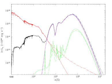
Figure 1: The SEDs of two models corresponding to ARP220 with a geometry of a King sphere. Dashed lines are for GRASIL, while continuous lines are for GRASIL-3D operating on a Monte Carlo realization of the same model, see text. The black lines are the final SEDs when dust effects are taken into account, the dashed blue and continuos magenta lines correspond to extinguished MCs emission (for GRASIL and GRASIL-3D, respectively), green to cirrus emission, and red to stellar emission when the dust effect is not taken into account.

3.2 GRASIL-3D versus GRASIL Results

As GRASIL-3D is based on the formulism of GRASIL (with slightly different dust model implementations), comparing the SEDs they produce when applied to the same galaxies is a necessary check for GRASIL-3D.

To this end, we have produced analytical galaxy models to be compared with GRASIL results. They are Monte Carlo realizations with $N_{part}$ particles of King spheres (see S98) and Monte Carlo realizations of SFR histories. More specifically, following S98 we have built a Monte Carlo model for ARP220 with a core radius $r_{c}=0.5$ kpc, an age of 13 Gyr, where the SFRH $\phi(t)$ is constant in the interval of the age of the Universe 1 Gyr $<t_{u}<$ 12.95 Gyr, involving a stellar mass of $2.3\times 10^{11}M_{\odot}$. Later on, for 12.95 Gyr $<t_{u}<$ 13 Gyr it undergoes an exponential burst with e-folding time $t_{e}=0.05$ Gyr involving a gas mass of 2.5 $\times 10^{10}M_{\odot}$. The gas mass fraction at $t_{u}=$ 13 Gyr is $f_{gas}=$ 0.139, the fraction of gas in molecular clouds is assumed constant at $f_{mc}$=0.5 and the parameter regulating the escape of young stars from MC is $t_{0}=$50 Myr, with a solar metallicity and molecular cloud radii of $r_{mc}=10.6$ pc.

In Figure 1 we show the SEDs for this model, calculated with both GRASIL-3D and GRASIL. Taking into account the differences of the dust model implementation, that mainly affect the cirrus and in particular their PAH emission (see discussion in V05), the agreement can be considered very satisfactory. Note that the difference in the intrinsic stellar emission appears because the reported GRASIL computation (dashed red line) includes the emission from dust in the stellar envelopes directly into the stellar population models, following Bressan et al. (1998) and Bressan et al. (2002), while that of GRASIL-3D (full red line) does not.

4 Applications and Potentialities

GRASIL-3D has been interfaced with a variety of galaxies identified in cosmological hydrodynamic simulations. Here we show results of galaxies run with two different codes: P-DEVA and GASOLINE. We note that we are not able to make accurate statistical analyses yet, as we do not have a statistical number of high resolution galaxy simulations (in fact, no group currently has such a set). Indeed, all we currently can achieve is to show that by interfacing GRASIL-3D with simulations (whose validity has been otherwise proved, see below), we obtain results consistent with observational data.

4.1 Hydrodynamic Codes

4.1.1 P-DEVA

P-DEVA is an entropy-conserving AP³M-SPH code, an OpenMP parallel version of the DEVA code (Serna et al., 2003), which includes the chemical feedback and cooling methods described in Martínez-Serrano et al. (2008). The primary concern when developing this code was that conservation laws (e.g. momentum, energy, angular momentum and entropy) hold accurately (see Serna et al., 2003, for details). The star formation recipe implemented in the DEVA code follows a Kennincutt – Schmidt-like law with a given density threshold, $\rho_{*}$, and star formation efficiency $c_{*}$. In line with Agertz et al. (2011), inefficient SF parameters are implemented, which implicitly account for the regulation of star formation by feedback energy processes by mimicking their effects, which are assumed to work on sub-grid scales.

The chemical evolution implementation (Martínez-Serrano et al., 2008) accounts for the full dependence of the radiative cooling on the detailed composition of the gas, through a fast algorithm based on a metallicity parameter, $\zeta(T)$, which takes into account the weight of the different elements on the total cooling function. The code also tracks the full dependence of metal production on the detailed chemical composition of stellar particles (Talbot & Arnett, 1973), through a Q_ij formalism implementation of the stellar yields, for the first time in a SPH code. A probabilistic approach for the delayed gas restitution from stars reduces the statistical noise and allows for a detailed study of the inner chemical structure of objects at an affordable computational cost. Moreover, the metals are diffused in such a way as to mimic the turbulent mixing in the interstellar medium, and the radiative cooling depends on the detailed gas particles metal composition.

Hydrodynamic evolution leads to gas particles being either cold or hot, as gas temperature distribution in simulated galaxies has two conspicuous maxima. Stars mostly form from the cold component. As we have said above, the star formation history is directly provided by the simulation. Stellar particles are considered as SSPs, with given age, metallicity and IMF $\Phi(M)$, specifically a Salpeter IMF (Salpeter, 1955), with a mass range of [M_l,M_u]=[0.1,100]M_⊙. According to the chemical evolution scenario implemented in P-DEVA, stellar particles can be transformed into gaseous ones, according to a probabilistic rule.

Table 1: Data on the $z=0$ sample of simulated disk-like galaxies

Name	$m_{\rm bar}$	$M_{\rm star}$	$M_{\rm gas}$	SFR	$<Z_{\rm star}>$	$<Z_{\rm gas}>$	re	rs	B/D
	($10^{5}$ M⊙)	($10^{10}$ M⊙)	($10^{10}$ M⊙)	(M⊙/yr)	(10-2)	(10-2)	(kpc)	(kpc)
g1536_L∗	1.9	2.32	1.97	1.809	1.17	1.25	1.38	3.86	0.35
g21647	0.25	2.32	1.37	3.895	1.48	1.94	0.00	1.52	0.00
g7124	2.00	0.60	1.10	0.314	0.46	0.86	0.00	2.94	0.00
LD-5003A	3.82	1.66	0.39	0.550	1.77	2.47	0.28	2.72	0.39
HD-5004A	3.94	3.26	0.67	0.840	1.60	2.20	0.37	4.00	0.43
HD-5004B	3.94	3.05	0.86	0.986	1.52	1.96	0.26	3.29	0.30
HD-5103B	3.78	2.63	0.46	0.820	1.92	3.07	0.55	3.90	0.72
LD-5101A	3.79	1.29	0.33	0.622	1.65	1.99	0.32	3.83	0.19

4.1.2 GASOLINE

The GASOLINE galaxies are cosmological zoom simulations with initial conditions derived from the McMaster Unbiased Galaxy Simulations (MUGS, Stinson et al., 2010).

When gas becomes cool ($T<15000$ K) and dense ($n_{th}>9.3$ cm^-3), it is converted to stars according to a Kennincutt – Schmidt-like law with the star formation rate $\propto\rho^{1.5}$. Stars feed energy back into the surrounding gas. Supernova feedback is implemented using the blastwave formalism (Stinson et al., 2006) and deposits $10^{51}$ erg of energy into the surrounding medium at the end of the stellar lifetime of every star more massive than 8 M_⊙. Energy feedback from massive stars prior to their explosion as SNe has also been included (Stinson et al., 2013, as part of the MaGICC project). To mimic the weak coupling of this energy to the surrounding gas (Freyer et al., 2006), we inject pure thermal energy feedback, which is highly inefficient in these types of simulations (Katz, 1992; Kay et al., 2002). We inject 10% of the available energy during this early stage of massive star evolution, but 90% is rapidly radiated away, making an effective coupling of the order of 1%.

Ejected mass and metals are calculated based on the Chabrier IMF (Chabrier, 2003) and are distributed to the nearest neighbor gas particles using the smoothing kernel (Stinson et al., 2006). Literature yields for SNII (Woosley & Weaver, 1995) and SNIa (Nomoto et al., 1997) are used. Metals are diffused by treating unresolved turbulent mixing as a shear-dependent diffusion term (Shen et al., 2010), allowing proximate gas particles to mix their metals. Metal cooling is calculated based on the diffused metals.

4.2 Disk Galaxies

4.2.1 Simulated Disk Galaxies

In this case, simulations use the cosmological ”zoom-in” technique, with high-resolution gas and dark matter in the region of the main object. The cosmological parameters of a $\Lambda$CDM model were assumed for P-DEVA (GASOLINE) runs ($\Omega_{\Lambda}=0.723(0.760)$, $\Omega_{m}=0.277(0.240)$, $\Omega_{b}=0.04(0.04)$, and $h=0.70(0.73)$), in a 10 Mpc (64 Mpc) per side periodic box.

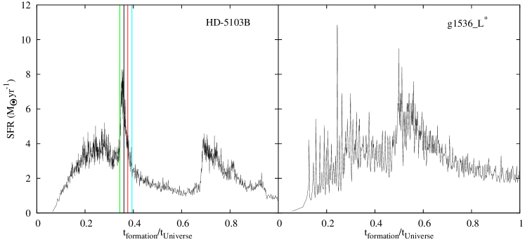
Figure 2: Left-hand panel: the stellar age distribution at $z=0$ for the disk galaxy HD-5103B from Doménech-Moral et al. (2012), where color vertical lines mark the snapshots where this starbursting period will be analyzed in Section 4. Right-hand panel: the same for the g1536_L^∗ galaxy from MAGICC runs (Brook et al., 2012).

As a first application, the SED of the HD-5103B galaxy, analyzed by Doménech-Moral et al. (2012), has been calculated and analyzed at $z=0$. Moreover, the SEDs and colors of HD-5103B around one of its star-forming major mergers have been carefully studied and compared to the phase of milder SF activity at $z=0$. To compare with currently available data on local, non-starbursting spiral galaxies, see $\S$4.4.1 below, we have also analyzed 4 more galaxies run with P-DEVA (LD-5003A, HD-5004A, HD-5004B, LD-5101A, see Doménech-Moral et al., 2012), as well as 3 galaxies run with GASOLINE from the MAGICC project (g1536_L^∗, g21647, g7124, see Brook et al., 2012; Stinson et al., 2013). Except for g21647 and g7124 galaxies, first analyzed by Obreja et al. (2014, submitted to MNRAS), these galaxies have all previously appeared in the literature, where more details can be gathered. The choices of most of the relevant parameters to run the P-DEVA simulations, as well as many of those characterizing the galaxies properties, are summarized in Tables 1 and 2 of Doménech-Moral et al. (2012) and in Table 1 of Obreja et al. (2013).

An important parameter here is the softening, setting the grid cell size. The gravitational softening used in the 5 P-DEVA runs is $\epsilon_{g}=400h^{-1}$ pc, while $\epsilon_{g}=312,5$ pc for g1536_L^∗ and g7124, and $\epsilon_{g}=156,2$ pc for g21647 galaxies. Some properties of the $z=0$ galaxies, provided by the simulations and some of them relevant to GRASIL-3D SED calculation, are given in Table 1. We see that both the SFR (averaged over the past 100 Myrs) and the specific SFR are low, that the disk and bulge scalelengths, and the bulge-to-disk luminosity ratios are consistent with observations, as other galaxy properties previously analyzed (see, for example Doménech-Moral et al., 2012; Stinson et al., 2013). The images of these galaxies (see for example Figure 6 for g1536_L^∗ or Figure 1 in Doménech-Moral et al., 2012) show that they are not interacting galaxies, as defined for example by Smith et al. (2007) or Lanz et al. (2013), see $\S$ 4.4.1 below. Therefore, these 8 galaxies can be considered as local normal galaxies, with low or very low starbursting activity, and hereafter will be refereed to as the $z=0$ sample of normal simulated disk-like galaxies.

More details on this $z=0$ sample of simulated disk-like galaxies provided by GRASIL-3D can be found in Table 3, and on HD-5103B during its starbursting phase in Table 6. Results in both Tables will be discussed later on.

To calculate the SED of a galaxy, a crucial piece of information is its stellar age distribution. They are provided in Figure 2 for HD-5103B and g1536_L^∗, where we can see that HD-5103B has been involved in two major merger events during its assembly process, with starbursting activity. The first starbursting phase will be analyzed in detail in $\S$4.4.2 as a model for a system with relatively high SF activity. .

Note that to transform from stellar age distribution to star formation rate, needed to calculate stellar luminosities, we corrected for gas restitution applying the Lia et al. (2002) formalism (see also Martínez-Serrano et al., 2008).

Figure 3: The stellar age distribution at $t_{\rm formation}/t_{\rm Universe}=0.1113$ of the high $z$ galaxy, D-6254, identified in the simulation #7629.

4.2.2 The Parameter Space and its Validation

The allowed ranges of parameter values in GRASIL-3D have been discussed in Section 2.6. More specifically, in Table 2 we give the combinations of parameters we used for studying the $z=0$ sample of normal simulated disk-like galaxies (those marked N in column 2), as well as the starbursting phases of HD-5103B (marked S in column 2). Each parameter set is identified by its name (first column) and a symbol in Figure 8.

Table 2: The parameter combinations used to test GRASIL-3D on simulated disk galaxies, either in starbursting phases (S) or in normal (N) ones

Set	Phase	$t_{0}$	$\rho_{mc,thres}$	$\sigma$
		(Myrs)	(M⊙kp-3)
		$r_{mc}=$14 pc
1	N	2.5	3.3$\times 10^{9}$	3
2	N	2.5	3.3$\times 10^{9}$	2
3	N	2.5	3.3$\times 10^{8}$	3
4	N	5	3.3$\times 10^{9}$	3
5	N	5	3.3$\times 10^{9}$	2
6	N	5	3.3$\times 10^{8}$	3
7	N, S	10	3.3$\times 10^{9}$	3
8	N, S	10	3.3$\times 10^{9}$	2
9	N, S	10	3.3$\times 10^{8}$	3
10	S	40	3.3$\times 10^{9}$	3
11	S	40	3.3$\times 10^{9}$	2
12	S	40	3.3$\times 10^{8}$	3
		$r_{mc}=$17 pc
13	N, S	10	3.3$\times 10^{9}$	3
14	N, S	10	3.3$\times 10^{9}$	2
15	N, S	10	3.3$\times 10^{8}$	3

To make identification easier, the table is divided by a double horizontal line, and each part is further divided by simple horizontal lines. The difference between the sets belonging to the upper and lower Table blocks are the parameters characterizing individual MCs, namely their radii $r_{mc}$, entering in the calculation of their optical depth, now a local quantity (see Eqs. 20 and 13). Parameter sets separated by single horizontal lines have different $t_{0}$ values (we recall that this parameter sets the fraction of light that can escape the starburst regions, mimicking MC destruction by young stars, see Section 2.2.6).

Finally, the three parameter sets within each sub-block differ in the parameters setting the molecular mass (and cirrus) fraction at each grid cell, namely the threshold density for MC formation and the dispersion in the PDF, $\rho_{mc,thres}$ and $\sigma$ respectively. They also set the global MC and cirrus mass, as well as the global MC fraction, $f_{mc}$, and through the cirrus mass, the total amount of dust in cirrus.

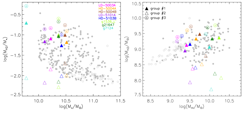
Figure 4: Comparison of molecular and atomic hydrogen content and stellar masses of the simulated sample of disk galaxies at $z=0$ to those of galaxies in the COLD GASS survey (Saintonge et al. 2011). Different color symbols distinguish different objects according to the coding in the left-hand panel. Filled, open and composed symbols correspond to parameter Sets # (1,4,7,13), (2,5,8,14) and (3,6,9,15), respectively, these three groups giving degenerated results in these plots. Gray points are data, with open symbols corresponding to non-detections (upper limits). For details see Saintonge et al. (2012) and Figures 5 and 8 therein.

The models in Table 2 explore the entire range of allowed values for the $t_{0}$ parameter ($t_{0}\sim$ 2.5 - 8 Myrs for normal spiral galaxies, and $t_{0}\sim 18-50$ Myrs for starbursting ones, according to S98), as well as the range for the $\rho_{mc,thres}$ and $\sigma$ parameters. Regarding these last two: i), the extreme values of $\rho_{mc,thres}$ are 10 - 100 H nuclei cm${}^{-3}\approx 3.3\times 10^{9}-3.3\times 10^{8}M_{\odot}\times kpc^{-3}$ taking a H nuclei-to-gas mass ratio of 0.75, and ii), for the dispersion of the log-normal PDF we have also taken its extreme values found in literature, $\sigma=3$ and $\sigma=2$. This would give 4 combinations describing extreme range values for the parameters governing the calculation of $f_{mc}$. It turns out that the combinations ($\rho_{mc,thres}=3.3\times 10^{9}M_{\odot}kpc^{-3},\sigma=3$) and ($\rho_{mc,thres}=3.3\times 10^{8}M_{\odot}kpc^{-3},\sigma=2$) give similar results, and therefore we have not shown the last.

As discussed in $\S$2.4, only the $\rho_{mc,thres}$ and $\sigma$ parameters affect the MC content of a given galaxy. Indeed, in Table 6 the degeneracies among parameter Sets relative to masses of molecular and atomic hydrogen of simulated galaxies are clearly shown. In fact, using parameter Sets belonging to each of the following three groups # (1,4,7,13), # (2,5,8,14) and # (3,6,9,15), gives the same MC and cirrus content. Hereafter they will be named groups #1, #2 and #3 of parameter Sets, respectively.

An important and necessary consistency test for these choices is to compare the resulting masses of molecular and atomic hydrogen of simulated galaxies to observational data. This has been done in Figure 4 for local galaxies, where gray symbols are data on local galaxies taken from Saintonge et al. (2012), and color symbols correspond to the sample of 8 $z=0$ simulated disk-like galaxies described above, see also Table 3 for parameter Set 4. More information on the MC content of some of the simulated galaxies can be found in Table 6 for the different parameter Sets, where we see that the mass in their MC content increases when $\sigma$ increases, from group #2 of parameter Sets to group #1, and increases more again when $\rho_{mc,thres}$ is reduced from 3.3 $\times 10^{9}$ M_⊙kp^-3 in group #1 to 3.3 $\times 10^{8}$ M_⊙kp^-3 in group #3.

Then, in Figure 4, we see that group #2 of parameter Sets results in too little molecular gas for the three galaxies run with GASOLINE (open green and turquoise triangles outside the data cloud), as well as for the LD-5101A one run with P-DEVA. Therefore group #2 of parameter Sets will not be further used in this paper for these galaxies. However, the extreme $f_{mc}$ values provided by group #2 and group #3 are within the range of observations for the other galaxies. Overall, of the 3 models in Figure 4 we see that the parameter Sets within group #1 give the best (and comfortably good) consistency with Saintonge et al. (2012) data of local galaxies. We also note that the stellar mass of g7124 is outside the rage of stellar masses in Saintonge et al. (2012).

As remarked in $\S$2.6, PHIBSS survey on $z\sim 1-3$ massive galaxies ($M_{*}\geq 10^{10.4}$) by Tacconi et al. (2013), provides new data on their molecular content. An extrapolation to lower masses is provided by their Figure 12, to be compared to our results in Table 6 for the merging phase of HD-5103B. The consistency is good for starburst galaxies. We conclude that the values used for $\rho_{mc,thres}$ and $\sigma$ adequately describe the molecular cloud content of simulated disk galaxies.

Regarding other parameters, we note that the values of both the time young stars remain enshrouded in MCs ($t_{0}=2.5$ Myrs, parameter Sets 1 - 3, $t_{0}=5$ Myrs, parameter Sets 4 - 6, and 10 Myrs, parameter Sets 7 - 9), and the masses and radii of molecular clouds ($m_{mc}=10^{6}$M_⊙ and $r_{mc}=14$pc) we have used are typical of normal spiral galaxies according to the discussion in Section 2.6. We have also used a value of $t_{0}=40$ Myrs, more typical of starburst galaxies, to test the star-forming phases of these galaxies (parameter Sets 10, 11 and 12). Values of $t_{0}=10$ Myrs in combination with a molecular cloud radius $r_{mc}=17$ pc (parameter Sets 13, 14 and 15) have been used to find out the effects of having a smaller optical depth in MCs (see Eq. (31)). The effects of GRASIL-3D parameter variations on the SEDs of simulated galaxies will be further discussed in Section 5.

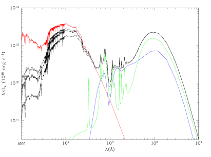
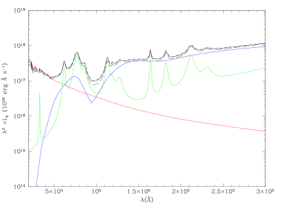
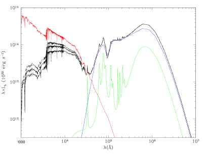
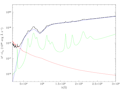
Figure 5: The rest-frame SEDs of disk galaxy HD-5103B at $z=0$ calculated with parameter Set 4 (top left) and of starburst D-6254 with parameter set SB7 (bottom left), and the zooms in the PAH band region of the rest-frame emitted fluxes of HD-5103B (top right) and D-6254 (bottom right). The color code for the lines is the same as in Figure 1, with the upper (lower) black line corresponds to the face-on (edge-on) view of the galaxies, while the middle black line is the angle-averaged emission.

Table 3: Masses, luminosities and energy balances (in parentheses) for the sample of $z=0$ disk-like galaxies calculated with parameter Set # 4

Name	Young Stars	Free Stars	MCs	Dust in Cirrus	$L_{bol}$	$L_{c}$	$L_{mc}$
	($10^{6}M_{\odot}$)	($10^{10}M_{\odot}$)	($10^{10}M_{\odot}$)	($10^{7}M_{\odot}$)	($10^{44}$ erg sec-1)	($10^{44}$ erg sec-1)	($10^{44}$ erg sec-1)
g1536_L∗	18.269	2.3188	0.2312	9.5034	1.7857 (97.9)	0.4948 (98.4)	0.5506 (92.2)
g21647	46.906	2.3171	0.2155	9.5589	3.2408 (99.4)	1.2932 (96.9)	1.2597 (96.5)
g7124	7.4456	0.5959	0.1169	3.8345	0.5922 (94.6)	0.0715 (99.3)	0.2448 (87.1)
LD-5003A	6.4977	1.6624	0.1346	2.8819	0.4676 (99.9)	0.1197 (98.2)	0.1019 (94.2)
HD-5004A	8.2845	3.2545	0.2140	4.2582	0.8334 (99.2)	0.2413 (98.4)	0.1629 (95.0)
HD-5004B	10.651	3.0469	0.3023	4.5436	0.8426 (99.6)	0.2561 (99.4)	0.1761 (94.2)
HD-5103B	4.9310	1.2906	0.0889	2.1182	0.4090 (100)	0.0739 (96.7)	0.0681 (93.6)
LD-5101A	6.0475	2.5362	0.1433	4.0385	0.7864 (98.8)	0.2303 (98.7)	0.1471 (97.8)

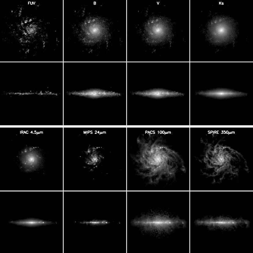
Figure 6: Face-on and edge-on images of the g1536_L^∗ galaxy at redshift $z=0$ in the 8 bands specfied in each panel. The physical size of each panel is 50 kpc per side. No telescope effects (like point-spread functions, pixel sizes, etc) have been taken into account.

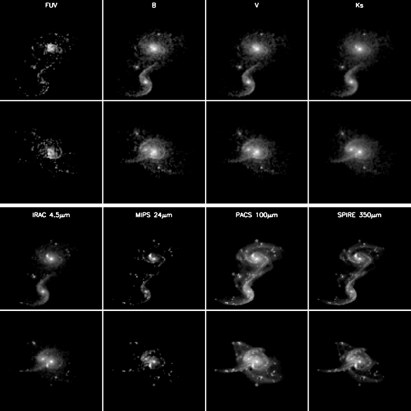
Figure 7: Two orthogonal views of a triple merger at $z=0.28$ involving disk galaxies giving rise to HD-5103B spiral at $z=0$. The 8 bands specfied in each panel are the same of the previous Figure. The physical size of each panel is 45 kpc per side. No telescope effects (like point-spread functions, pixel sizes, etc) have been taken into account.

4.2.3 The SEDs and Luminosities of Simulated Disk Galaxies

To demostrate how the SEDs of simulated galaxies look, in Figure 5 we show the SED of HD-5103B disk galaxy (top left) and a zoom of the corresponding emitted flux in the MIR region (top right), where the PAH band emission stands out. This SED has been calculated using the fiducial dust model described in Section 2.4 and the parameter Set 4 given in Table 2. Their color code is similar to that in Figure 1, with the upper (lower) black lines corresponding to the face-on (edge-on) view of the galaxies, while the middle black line is the angle-averaged emission. We can see in Figure 5 that, as expected, the difference between the face-on and edge-on views is remarkable in the UV and at optical wavelengths, while it is unimportant at longer ones. The comparison of these SEDs to observations will be analyzed in $\S$4.4.

Other important data on simulated galaxies returned by GRASIL-3D, appart from those shown in Figure 4, are the total bolometric luminosity, $L_{bol}$, and the total cirrus and molecular cloud emmitted energy, $L_{c}$ and $L_{mc}$, respectively. These can be found in Table 3 for the $z=0$ sample of normal simulated disk-like galaxies, along with their respective energy balances. We see that the luminosities are consistent with observations (see $\S$4.4 below), and that the balances are generally very good.

4.3 Simulated Disk and Merger Images

In Figure 6 we show face-on and edge-on images of the g1536_L^∗ galaxy at redshift $z=0$ in 8 bands going from far-UV to FIR. From left to right and from top to bottom, they correspond to GALEX (FUV), Johnson (B and V), 2MASS (Ks), IRAC (4.5 $\mu$m), MIPS (24 $\mu$m), PACS (100 $\mu$m) and SPIRE (350 $\mu$m) bands. The physical size of each panel is 50 kpc per side. Note the clumpy appearence in the UV and IR bands, as compared with the other bands. The effects of dust obscuration are clear in the edge-on images, and particularly so in the B and V bands where dust lanes can be appreciated accross the disk. Bright spots are star formation regions, nicely visible on the spiral arms.

GRASIL-3D is very useful to study mergers of simulated galaxies, where geometries can be very complex. As an illustration, in Figure 7 we show two orthogonal views of a triple merger of disk galaxies at $z=0.28$, giving rise to the HD-5103B spiral at $z=0$. The bands are the same as in the previous Figure (rest-frame emission). In this case the panels correspond to 45 kpc per side. Again, the UV and IR emission are more clumpy than the other bands. Note that in one of the perspectives, tidal tails (where IR emission concentrated in knots corresponds to star formation bursts) look very similar to those observed in the local Antennae merger, while in the other the spiral structure of one of the galaxies is still visible.

4.4 Comparing GRASIL-3D SEDs of Disk Galaxies to Observations

It is important to know how well the SEDs of simulated galaxies behave as compared to observational data. We are particularly interested in the rest-frame near-IR region up to the far-IR, where the effects of cirrus and MC emission dominate. Comparisons with data coming from different projects are discussed in turn, taking into consideration the starbursting/quiescent SF phase and/or the interacting/non-interacting situation of simulated and real galaxies.

4.4.1 Observational Data to Compare with

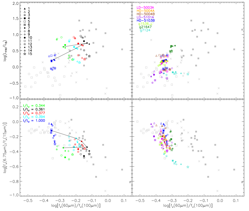
Figure 8: Upper-left panel: The rest-frame FIR/blue luminosity ratio $L_{\rm FIR}/L_{\rm B}$ versus the rest-frame IRAS flux density ratios f_ν(60$\mu$m)/f_ν(100$\mu$m) for the HD-5103B galaxy at $z=0$ (blue) and at different times around one of its major mergers, according to the color code in the lower left-hand panel. Different symbol shapes distinguish different parameter sets (see Table 2) as encoded on the left of this panel. Gray points are the same ratios for the Dale et al. 2000 sample shown for comparison, where the filled and empty squares represent FIR-active (i.e., starbursting galaxies) and FIR-quiescent objects, while crosses are intermediate systems (mild starbursts), according to the classification of Vega et al. 2005. Lower-left panel: Same as in the upper panel for the f_ν(6.7$\mu$m)/f_ν(15$\mu$m) vs the f_ν(60$\mu$m)/f_ν(100$\mu$m) flux ratios. Black lines in these two panels join consecutive parameter Set 7 results for the HD-5103B galaxy at its starburst phases and the Set 4 result for the quiescent phase at $z=0$. The right-hand panels are similar to those at their left for the whole sample of 8 $z=0$ simulated normal disk-like galaxies, whose identity is encoded by the colors at the left of this panel. Face-on emissions have been used to draw this Figure.

The following observational samples and projects are used as reference:

1. ISO Key Project on the ISM of Normal Galaxies (Helou et al., 1996). Dale et al. (2000) provide ISO and IRAS broad-band fluxes. Based on the Lu et al. (2003) definition of stellar activity, V05 classify these galaxies into FIR-active (i.e., starbursting, with log[L_FIR/L_B] $\geq 0$ and log[f_ν(60$\mu$m)/f_ν(100$\mu$m)] $\geq-0.24$, 43% of the sample), FIR-quiescent (with no or very low SF, log[L_FIR/L_B] $<0$ and log[f_ν(60$\mu$m)/f_ν(100$\mu$m)] $<-0.24$, 31% of the sample) and FIR-intermediate (mild SB phases, 26% of the sample), see their Figure 3.

2. Lu et al. (2003) sample: a subsample of Dale et al. (2000) where the aromatic features in emission (hereafter AFEs) at 6.2, 7.7, 8.6, and 11.3 $\mu$m dominating the mid-infrared (MIR) are analyzed in detail. In addition, Lu et al. provide their ISOPHOT spectra.

3. The Spitzer IR Normal Galaxy Survey (SINGS), see Kennicutt et al. (2003) and Dale et al. (2005): 75 local galaxies with different morphologies with Spitzer data. By removing SINGS galaxies with close companions, Smith et al. (2007) have selected a sample of 42 non-tidally perturbed galaxies (their non-interacting sample; 26 spirals, 4 E+SO, 12 Irr/Sm galaxies). A subsample of these galaxies using a more conservative definition for being non-interactive is listed in Table 10 of Lanz et al. (2013) (as part of the KINGFISH project).

4. The Herschel project on Key Insights on Nearby Galaxies: Far Infrared Survey with Herschel (KINGFISH, Kennicutt et al., 2011), which consists of 61 galaxies where 57 are SINGS galaxies. They are subluminous IR galaxies and all normal galaxy types are represented. All were imaged with Herschel PACS and SPIRE (Dale et al., 2012), including those listed by Lanz et al. (2013) as non-interactive.

4.4.2 Results

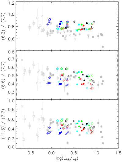
Figure 9: The relative strengths of the AFEs as a function of the FIR/blue luminosity ratio for the HD-5103B galaxy at $z=0$ (blue) and at different times around one of its major mergres. The color and shape codes are the same as in Figure 8 (left-hand panels), with the gray points (filled and empty squares, and crosses) representing the observational sample of Lu et al. 2003, according to their nature (FIR-active, FIR-quiescent and intermediate, respectively).

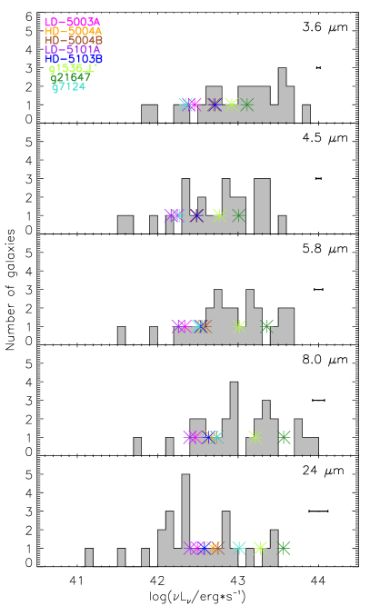
Figure 10: Comparison of fluxes in different Spitzer IRAC and MIPS bands for non-interacting normal disk-like galaxies. The histograms have been drawn with data for the sample of 26 non-interacting galaxies from Smith et al. (2007), Tables 2 and 6, selected from SINGS galaxies, see text. Points stand for the sample of 8 disk-like simulated $z=0$ galaxies, their identity is encoded by colors as in previous Figures. Plotted are averages over results as model parameters take their allowed values (Table 2 for N phase). The error bars at the right of each panel give the maximum dispersions over the 8 simulated galaxies.

As most of these projects provide us just with photometric data (i.e., no spectra), rather than a direct comparison of SEDs, an appropriate method to compare calculated SEDs with observed ones comes from fluxes, colors or flux ratio comparisons. As a first exercise, we have made comparison to IRAS and ISOCAM results on normal local galaxies, i.e., the Dale et al. 2000 sample, classified by V05 according to their SFR activity, see (i) in $\S$4.4.1 above. In Figure 8 we plot the FIR/blue luminosity ratio $L_{\rm FIR}/L_{\rm B}$ versus the IRAS 60 $\mu$m/ 100 $\mu$m flux density ratio, for the Dale sample (in gray) with different symbols standing for starbursting/FIR-active, mildy starbursting/FIR-intermediate and FIR-quiescent galaxies.

To test the ability of GRASIL-3D to return observational results for starbursting galaxies, the HD-5103B starbust period around $t/t_{U}\sim 0.35$ has been analyzed in detail by plotting its different phases in Figure 8, upper panel at the left, and comparing them with the situation at $z=0$, where the SF activity is milder. The different colors distinguish different starburst phases. More specifically, green, black, red, and cyan correspond to $t/t_{U}$ = 0.344, 0.361, 0.377, and 0.394, respectively. In Figure 2 we see that they correspond to the beginning of the starburst phase, two snapshots along the active phase (in black and red), and its end, respectively. We also plot these ratios for the HD-5103B at $z=0$ (blue). Different symbols in the simulated galaxies stand for different parameter Sets, according to the code in the panel and to Table 2. Results for the different models in this Table have been drawn in Figure 8 to illustrate their dispersion due to parameter variation within their allowed ranges (note that parameter Sets with $t_{0}=40$ Myrs are excluded for $z=0$ galaxies). To highlight the time evolution, in Figure 8 those points corresponding to parameter Set #7 (#4) in the starburst (quiescent) phases have been connected by a black line.

We see that these results are consistent with observational results. When compared to Figure 3 in V05, for example, the black, red and cyan points correspond to FIR-active (starbursting) galaxies, irrespective of the GRASIL-3D parameter set we use, while the green points fall in the observational range for FIR-intermediate (mild starbursts) galaxies, and the blue points in that of either FIR-intermediate or quiescent galaxies. It is worth noting that, as expected, the most FIR-active galaxy phases among those analyzed correspond to the black symbols, that is, just at the time when the starburst in Figure 2 is at the top of its star formation activity. Moreover, as the black line highlights, the time evolution is also as expected. It causes a correlation between the $L_{\rm FIR}/L_{\rm B}$ and the IRAS 60 $\mu$m/ 100 $\mu$m flux density ratios as Figure 8 clearly shows.

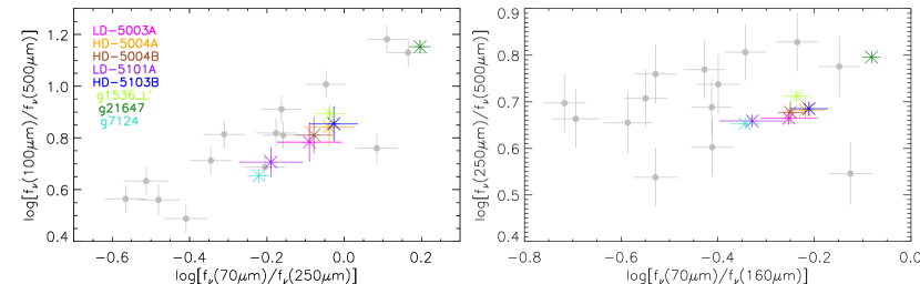
Figure 11: Comparison of some flux density ratios in Herschel bands for the $z=0$ sample of simulated disk-like galaxies (colors) to the corresponding ratios for the non-interacting local spiral galaxies selected by Lanz et al. 2013 (gray symbols). Simulated points are averages over results as model parameters take their allowed values (Table 2 for N phase), and error bars stand for their dispersions.

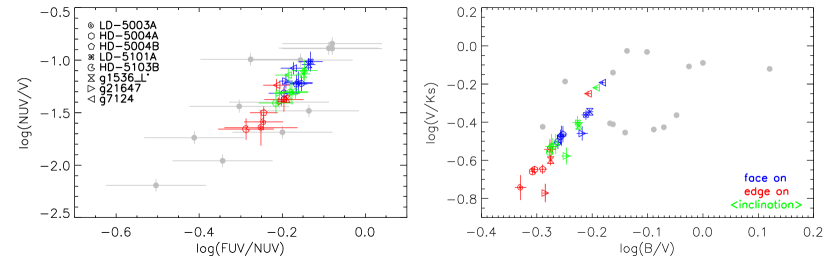
Figure 12: UV and optical flux density ratios plots for the sample of $z=0$ simulated normal disk-like galaxies averaged over parameter sets, with their corresponding dispersions, in comparison to the sample of non-interacting galaxies from Lanz et al. (2013, grey points). Data are from Dale et al. (2007), where no error bars are provided for the flux density ratios shown in the right-hand panel. Colors stand for different disk orientations: face-on (blue), edge-on (red) and angle-averaged (green).

To emphasize the correctness of GRASIL-3D results regarding the location of normal non-starbursting disk galaxies in this plot, results for the whole sample of simulated $z=0$ disk galaxies described in Section 4.2 are shown in Figure 8 upper right-hand panel. In this case, colors distinguish galaxy identities, as specified in the left of the panel, while symbol shapes mean different parameter Sets, as above. We see that these non-starbursting disk-like galaxies show flux density ratios characteristic of FIR-quiescent or intermediate galaxies, according to V05 classification.

To further probe the capability of GRASIL-3D to describe starbursting against more quiescent galaxies, in Figure 8, lower panel on the left, the f_ν(6.75$\mu$m)/f_ν(15$\mu$m) flux ratios are plotted against f_ν(60$\mu$m)/f_ν(100$\mu$m). Symbol shapes or colors have the same meaning as in the upper left-hand panel. This plot can be directly compared with Figure 4 of V05. A good consistency of simulations with the observational data can be appreciated regarding the location of the quiescent $z=0$ phase and the starbursting ones relative to observational points. Moreover, when the different snapshots around the HD-5103B galaxy merger are considered, the motion of the color-color representative points in the plane follows trajectories (i.e., the black line) consistent with those shown in Figure 4 of V05, once we take into account the much higher complexity of the merger for simulated galaxies as compared to the models plotted in V05 .

Figure 8, lower panel on the right, shows the same flux ratios as shown in the left, in this case for the entire sample of simulated $z=0$ disk-like galaxies. We see that the consistency is mostly good relative to non-starbursting galaxies in Dale (2000) sample.

Summing up, the four panels in Figures 8 demostrate that GRASIL-3D is a good tool to calculate the SED of galaxies in different phases of their SF activity, including the wet merger sequence causing the starbursts. Indeed, its capability in these tasks is comparable to GRASIL.

As mentioned above ($\S$4.4.1 point (ii)), Lu et al. (2003) provide ISOPHOT spectra for a sample of 45 disk galaxies from the same ISO Key Project on Normal Galaxies, providing their average stacked spectra. They analyze the AFEs at 6.2, 7.7, 8.6, and 11.3 $\mu$m dominating the mid-infrared (MIR). Note the remarkable similarity between their average rest-frame spectra (Lu et al., 2003, Figure 3) and those shown in Figure 5 upper panel on the left and its $F_{\nu}$ zoomed version.

Therefore, another possible interesting comparison with observational results is provided by the relative strengths of the rest-frame AFEs for this same sample (Lu et al. 2003, Figure 8 and Table 6). For the five snapshots analyzed in the HD-5103B galaxy they are shown in Figure 9. The agreement is good and it supports these authors’ main claim, namely that the dispersion in the AFE ratios is low for their sample (in the case of simulated results, this is particularly true when GRASIL-3D parameter sets are individually followed), and that little correlation is seen between their variations and either the IRAS f_ν(60$\mu$m)/f_ν(100$\mu$m) flux density ratios or the FIR/blue luminosity ratios (i.e., galaxy SF phase activity). Not shown in the Figure are the relative strengths of the AFEs corresponding to the entire z=0 sample of normal simulated disk-like galaxies, these relative strengths are compatible with those corresponding to FIR-quiescent and intermediate observed galaxies.

The galaxies in the Spitzer Infrared Nearby Galaxies Survey (SINGS, see Dale et al., 2005, 2007, and point (iii) in $\S$4.4.1) constitute an essential reference sample to compare with the IR emission of any calculated SEDs. In this case, a subsample of non-interacting galaxies is available (Smith et al., 2007), allowing us to make comparisons separately.

We have therefore calculated the IRAC and MIPS flux ratios at 3.6, 4.5, 5.8, 8.0, 24, 70 and 160 $\mu$m for our sample of $z=0$ disk-like galaxies. In calculating magnitudes at 3.6, 4.5, 5.8, 8.0 and 24 $\mu$m, we used zero points of 280.9, 179.7, 115.0, 64.1 and 7.14 Jy, respectively (IRAC Data Manual; MIPS Data Manual). In Figure 10 we show the fluxes in these 5 bands. Points are averages over results with different parameter Sets in Table 2 marked (N), and the flux histograms correspond to the sample of 26 non-interacting local galaxies analyzed in Smith et al. (2007). No color corrections were applied in calculating these fluxes. The agreement is good, proving that GRASIL-3D correctly returns fluxes in Spitzer filters for spiral galaxies.

A more restrictive selection of non-interacting galaxies from the normal galaxy sample of Smith et al. (2007) is provided by Lanz et al. (2013), see (iii) and (iv) in $\S$ 4.4.1. Figure 11 shows some FIR flux density ratio diagrams for our sample of 8 disk-like galaxies at $z=0$ and the corresponding flux density ratios for the observed ones. Again we see that the consistency is satisfactory, showing that GRASIL-3D gives sound results in Herschel bands.

Apart from the IR analysis, colors in the UV and optical wavelengths have also been analyzed, see Figure 12 where face-on, edge-on and angle-averaged disk orientations are shown separately for simulated galaxies. As shown by these plots, the comparison to non-interacting local spiral galaxies (Lanz et al., 2013) is satisfactory for the sample of $z=0$ disk-like galaxies.

As already mentioned, parameter changes within their allowed ranges have effects on the galaxy SEDs as well as on IRAS-ISO colors and AFE relative strengths. This will discussed in $\S$5.

4.5 A Starburst Galaxy at High z

A second very interesting potentiality of GRASIL-3D is its application to high-$z$ massive (multiple)-merging systems, picked in the fast phase of their assembly process (Domínguez-Tenreiro et al., 2006; Oser et al., 2010; Cook et al., 2009; Domínguez-Tenreiro et al., 2011). The timeliness of this application is reinforced by the fact that new observational facilities, such as Herschel and ALMA, observe at wavelengths where the IR emission maxima of these objects are shifted to, providing us with observational data to compare with, see for example Dowell et al. (2014), Hodge et al. (2013) and Decarli et al. (2014), among others.

One example of such systems is provided by the #7629 P-DEVA simulation, specifically designed to check GRASIL-3D when applied to such systems. In this simulation a box of 10 Mpc side has been sampled with $N_{DM}=256^{3}$ DM and $N_{bar}=256^{3}$ gas particles, and evolved using a spatial resolution of $\epsilon=400/h$ pc. The cosmological model corresponds to a flat $\Lambda$CDM with $\Omega_{\Lambda}$ = 0.72, $\Omega_{M}=0.28$, $\Omega_{bar}=0.046$ and $h=0.7$ (very similar to the cosmological parameters used in the disk runs). To have massive enough systems at high $z$s, a normalization of the initial perturbation field higher than usual has been used ($\sigma_{pert}=1.2$), therefore representing a dense subvolume of the universe, and the SF parameters have been taken as $\rho_{*}=3\times 10^{-25}$ g cm^-3 and $c_{*}=0.1$.

Different massive objects at high $z$s have been identified in the #7629 simulation. In this paper we focus on one of them labeled as D-6254. Its age distribution is given in Figure 3, showing that the object is a strong starburst. In Table 4 we give the GRASIL-3D parameter sets used in the SED analysis. Note that, again, those governing the molecular gas mass fraction $f_{mc}$ explore the entire range of their possible values, while $t_{0}$ and parameters setting the properties of individual MCs take values consistent with those S98 found for local starbursting galaxies (ARP220).

The corresponding gas mass and baryon fractions, $f_{mc}$ and $f_{mc,star}$ respectively, can be found in Table 6 where we see that, again, the mass in molecular clouds increases from parameter Sets SB5, SB8 and SB18 to Sets SB4, SB7 and SB17, as $\sigma$ increases from 2 to 3, and increases further for Sets SB6, SB9 and SB19, where $\rho_{mc,thres}$ decreases from 3.3$\times 10^{9}$ M_⊙kp^-3 to 3.3$\times 10^{8}$ M_⊙kp^-3. Moreover, if the conversion factor from the observed CO line flux to molecular gas mass is taken $\alpha\sim 1$ instead of $4.36$, as likely needed for starburst galaxies (Tacconi et al., 2013), then the values we found for the parameter Sets SB4 (SB7 and SB17) and SB6 (SB9 and SB19) are consistent with those found by these authors for massive galaxies between redshifts $z\sim 2.0-2.5$, the most distant where such analysis has been made so far. The molecular gas content corresponding to the parameter Set SB5 (as well as Sets SB8 and SB18) are too low.

The rest-frame SED of this object calculated with parameter Set SB7, as well as its zoom in the AFE region, are shown in Figures 5, bottom left- and right-hand panels, respectively. These two Figures illustrate that, as expected in a strong starburst object, the dust emission is dominated by MCs at any IR wavelength, and that, moreover, dust emission clearly dominates over the extinguished stellar emission at shorter wavelengths.

5 The effects of model parameters on the SEDs of simulated objects

Table 4: Different parameter sets used to analyze the effects of parameter variation on the D-6254 galaxy SEDs

Set	$t_{0}$	$\rho_{mc,thres}$	$\sigma$
	(Myrs)	(M⊙kp-3)
		$r_{mc}=$10.6 pc
SB4	20	3.3$\times 10^{9}$	3
SB5	20	3.3$\times 10^{9}$	2
SB6	20	3.3$\times 10^{8}$	3
SB7	40	3.3$\times 10^{9}$	3
SB8	40	3.3$\times 10^{9}$	2
SB9	40	3.3$\times 10^{8}$	3
		$r_{mc}=$17 pc
SB17	40	3.3$\times 10^{9}$	3
SB18	40	3.3$\times 10^{9}$	2
SB19	40	3.3$\times 10^{8}$	3

An important question is how the change of parameters in the model affects the SEDs of the different simulated objects we consider. To analyze this point, for each object different SEDs have been calculated by changing these parameters within their allowed ranges, see $\S$2.6 and Tables 2 and 4.

Table 5: Stellar masses, luminosities and energy balances (in parenthesis) of the HD-5103B galaxy at $z=0$ according to the different parameter sets in Table 2

Set code	Young Stellar	Free Stellar	$L_{bol}$	$L_{c}$	$L_{mc}$
	($10^{6}M_{\odot}$)	($10^{10}M_{\odot}$)	($10^{44}$ erg sec-1)	($10^{44}$ erg sec-1)	($10^{44}$ erg sec-1)
1	4.9136	2.5363	0.7871 (98.9)	0.2524 (99.56)	0.1164 (96.7)
2	4.9136	2.5363	0.7783 (97.8)	0.3172 (99.8)	0.1140 (98.8)
3	4.9136	2.5363	0.7934 (99.7)	0.1629 (99.0)	0.1165 (96.6)
4	6.0475	2.5362	0.7729 (99.5)	0.2334 (99.3)	0.1276 (96.9)
5	6.0475	2.5362	0.7665 (98.7)	0.3003 (98.4)	0.1252 (98.8)
6	6.0475	2.5362	0.7777 (99.9)	0.1462 (99.6)	0.1285 (96.3)
7	14.741	2.5353	0.7723 (99.5)	0.2094 (100.0)	0.1649 (97.9)
8	14.741	2.5353	0.7644 (98.4)	0.2740 (98.7)	0.1602 (99.2)
9	14.741	2.5353	0.7767 (99.9)	0.1270 (98.6)	0.1655 (97.6)
13	14.741	2.5353	0.7780 (99.8)	0.2103 (99.9)	0.1703 (94.8)
14	14.741	2.5353	0.7730 (99.6)	0.2759 (98.6)	0.1686 (95.8)
15	14.741	2.5353	0.7826 (99.2)	0.1274 (98.7)	0.1713 (94.2)

To properly interpret the results shown in Table 5, we recall that the total gas or stellar mass of a simulated galaxy, as well as its total bolometric luminosity in the absence of dust, are fixed by the simulation itself. Therefore, the sum of MC and cirrus total masses is fixed to the total gas mass, and the sum of the young and free stars is also fixed to the galaxy total stellar mass.

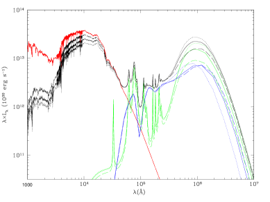
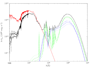
Figure 13: Comparison of the SEDs of the simulated galaxy HD-5103B at $z=0$ obtained under different parameter sets. Left-hand panel compares the effects of changing $\rho_{mc,thres}$ and $\sigma$, with full, point and dashed lines corresponding to code 4, 5 and 6 parameter Sets. Right-hand panel compares the effects of changing the $t_{0}$ parameter, with full, point and dashed lines corresponding to code 4, 1 and 7 parameter Sets. See Table 2 for parameter set values. Color line codes are as usual and only angle-averaged emissions are plotted.

5.1 The SEDs

As an illustration of the effects of parameter variations on the SED, in Figures 13 we show the SED of HD-5103B galaxy at $z=0$, calculated using parameter Sets 4, 5 and 6 (i.e., different $\rho_{mc,thres}$ and $\sigma$ values, left-hand panel) and parameter Sets 4, 1 and 7 (i.e., different $t_{0}$ values, right-hand panel). On the left-hand panel we see that increasing $f_{mc}$ (i.e., decreasing the cirrus fraction 5-4-6 parameter Sets), the dust absorption by cirrus in the UV and optical decreases, thereby decreasing the cirrus emission at longer wavelengths. The right-hand panel illustrates the consequences of increasing the time young stars remain within MCs: as $t_{0}$ increases from parameter Sets 1, 4, 7, the UV emission decreases, but the MC cloud emission increases, at the same time that the cirrus emission in the PAH region decreases.

5.2 The global masses and luminosities of the different galaxy components

As expected, Tables 6 and 5 show that the global masses of the different galaxy components are insensitive to $m_{mc}$ and $r_{mc}$ variations, and the global luminosities $L_{bol}$ and $L_{c}$ do not change. There is a tendency towards slightly higher values of $L_{mc}$ as $\tau_{mc}$ decreases.

Table 6: Galaxy HD-5103B at different $z$s, g1536_L^∗ at $z=0$ and D-6254 at $z=4$: Molecular Cloud and Cirrus Dust Content according to $\rho_{mc,thres}$ and $\sigma$

Group	Set	Molecular Clouds	$f_{mc}$	$f_{mc,star}$	Dust in Cirrus
		(1010 M⊙)			(107 M⊙)
			HD-5103B
		$t/t_{U}$ = 1	$M_{\rm tot}$ =2.973 $\times 10^{10}$ M⊙	$M_{\rm gas}=4.362\times 10^{9}$ M⊙
1	1, 4, 7, 13	0.1433	0.3286	0.0460	4.0385
2	2, 5, 8, 14	0.0257	0.0590	0.0100	5.8017
3	3, 6, 9, 15	0.2598	0.5956	0.0929	2.3493
		$t/t_{U}$ = 0.394	$M_{\rm tot}=1.397\times 10^{10}$ M⊙	$M_{\rm gas}=3.762\times 10^{9}$ M⊙
1	7, 10, 13	0.1674	0.4449	0.1409	1.1386
2	8, 11, 14	0.0855	0.2273	0.0773	1.9336
3	9, 12, 15	0.2423	0.6440	0.1918	0.5516
		$t/t_{U}$ = 0.377	$M_{\rm tot}=1.357\times 10^{10}$ M⊙	$M_{\rm gas}=3.771\times 10^{9}$ M⊙
1	7, 10, 13	0.1981	0.5253	0.1682	1.1156
2	8, 11, 14	0.1297	0.3439	0.1169	1.8727
3	9, 12, 15	0.2596	0.6886	0.2095	0.5573
		$t/t_{U}$ = 0.361	$M_{\rm tot}=1.295\times 10^{10}$ M⊙	$M_{\rm gas}=4.369\times 10^{9}$ M⊙
1	7, 10, 13	0.2773	0.6346	0.2441	0.9128
2	8, 11, 14	0.2127	0.4868	0.1986	1.5082
3	9, 12, 15	0.3328	0.7617	0.2794	0.4631
		$t/t_{U}$ = 0.344	$M_{\rm tot}=1.260\times 10^{10}$ M⊙	$M_{\rm gas}=5.586\times 10^{9}$ M⊙
1	7, 10, 13	0.3351	0.5998	0.3252	1.3797
2	8, 11, 14	0.1761	0.3153	0.2009	2.6681
3	9, 12, 15	0.4363	0.7811	0.3834	0.5958
			g1536_L∗
		$t/t_{U}$ = 1	$M_{\rm tot}=3.317\times 10^{10}$ M⊙	$M_{\rm gas}=1.082\times 10^{10}$ M⊙
1	1, 4, 7, 13	0.1750	0.1617	0.0726	6.1449
2	2, 5, 8, 14	0.0109	0.0101	0.0049	7.3175
3	3, 6, 9, 15	0.4039	0.3731	0.1530	4.5585
			D-6254
		$t/t_{U}$ = 0.110	$M_{\rm tot}=3.298\times 10^{10}$ M⊙	$M_{\rm gas}=7.293\times 10^{9}$ M⊙
1	SB4, SB7, SB17	0.3286	0.4506	0.1134	1.2033
2	SB5, SB8, SB18	0.1228	0.1684	0.0456	2.2805
3	SB6, SB9, SB19	0.4856	0.6656	0.1590	0.5395

The Tables also show that when $t_{0}$ increases, the global mass of young stars suffers an important increment in relative terms. The global mass of free stars decreases, but the effect is relatively less important. As a consequence, the total stellar energy to be processed by MCs increases, and, at the same time, the amount of stellar energy that directly heats the cirrus component becomes relatively less important. The resulting effect is that $L_{mc}$ increases, while $L_{c}$ decreases.

Regarding changes in $\rho_{mc,thres}$ and $\sigma$, we treat them in turn. When $\rho_{mc,thres}$ decreases, the global mass in MCs (and $f_{mc}$) increases, causing a decrement to the global gaseous mass in cirrus and to their dust content. A direct effect is that $L_{c}$ decreases. $L_{mc}$ keeps roughly constant, which can be understood as a consequence of the constant amount of energy from young stars heating the MC component.

The effects of $\sigma$ variations on the global masses and $L_{c}$ and $L_{mc}$ luminosities are in the opposite direction of those caused by $\rho_{mc,thres}$ changes, as can be seen in Tables 6 and 5. When both parameters vary, the effects can be somewhat compensated.

5.3 Flux density ratios

In this case, the major effects come from $f_{mc}$ value changes due to $\rho_{mc,thres}$ and $\sigma$ modifications, as illustrated by Figure 13. These effects are more apparent in the FIR/blue luminosity ratios shown in Figure 8, upper panels. Indeed, results corresponding to parameter sets bringing about degenerated $f_{mc}$ values, namely # (2, 5, 8, 11, 14; open symbols), # (1, 4, 7, 10, 13; filled symbols), and # (3, 6, 9, 12, 15; composed symbols), show up grouped together in FIR/blue luminosity ratios. According to Table 6, these groups of parameter sets correspond to increasing molecular gas content, and hence, to increasing L_B and decreasing cirrus emission in the FIR region. Indeed, in Figure 8 (top panels) we see that parameter Sets 2, 5, 8, 11 and 14 (not considered for GASOLINE galaxies) have the highest FIR/blue luminosity ratios. The effects are more important for FIR-active galaxies than for FIR-quiet phases, and they are within the data dispersion at given f_ν(60$\mu$m)/f_ν(100$\mu$m) ratios, that are much less affected by $f_{mc}$ variations.

The effects of changing the timescale for MC destruction, $t_{0}$, are not important on the FIR/blue luminosity ratios, $L_{\rm FIR}/L_{\rm B}$, and only modest on the IRAS 60 $\mu$m/ 100 $\mu$m flux density ratios, see Figure 8. Finally, changing the size of individual MCs corresponding to a 50% variation in their optical depth (Sets 13, 14 and 15 versus 7, 8 and 9), has no appreciable effects in Figure 8.

Other flux density ratios affected by changes in $f_{mc}$ are the IRAS-ISO 6.75 $\mu$m/ 14 $\mu$m flux ratios (Figure 8 lower panel) as well as the FUV/NUV and V/Ks flux density ratios, effects shown as error bars in Figure 12. Note however that the effects are consistent with the corresponding data dispersion. In this respect, we remind that $f_{mc}$ changes due to parameter variations are generally consistent with observational data on $f_{mc}$. In the case of parameter Set 5 (and 2, 8, and 14) the corresponding points in Figures 4 are at the limits of the data cloud of points or outside it.

Finally, it is remarkable to note that, as shown by Figures 8 and 9, the effects of modifying the $t_{0}$ or $r_{mc}$ parameters within their allowed ranges has insignificant effects in the disk flux density ratios analyzed in this paper.

These detailed analyses have been repeated for the D-6254 high-$z$ merger galaxy by comparing results obtained under parameter sets in Table 4, and the conclusions are similar to those reached for disk galaxies.

6 Summary, Discussion and Conclusions

In this paper we have introduced a new photometric SED code, GRASIL-3D, which includes a careful modelling of the radiative transfer through the dust component of the ISM. GRASIL-3D is an entirely new model based on the formulism of an existing and widely applied model, GRASIL, but specifically designed to be applied to systems with any arbitrarily given geometry, where radiative transfer through dust plays an important role, such as galaxies calculated by hydrodynamical galaxy formation codes.

A few codes exist that, by interfacing the outputs of hydrodynamic simulations, can Monte Carlo solve the radiative transfer through dust and therefore predict a multi-wavelength SED for simulated galaxies (SUNRISE, RADISHE, ART², see $\S$1). Following GRASIL, some GRASIL-3D particular strengths relative to these codes can be summarized as: i) the radiative transfer is not solved through Monte Carlo methods, but in a grid; ii) it is designed to separately treat radiative transfer in molecular clouds and in diffuse cirrus component, whose dust composition are different (for example, lower PAH fraction in MC dust); iii) correspondingly, it takes into account the age-dependent dust reprocessing of stellar populations (note that GRASIL has been the first model to do so), arising from the fact that younger stars are associated with denser ISM environments, mimicking through the $t_{0}$ parameter the time young stars are enshrouded within molecular clouds before their destruction; iv) it includes a detailed non-equilibrium calculation for dust grains with diameter smaller than $a_{flu}\sim 250$ Å, as required. This allows also a proper treatment of PAH features, dominating the MIR in some cases.

Current cosmological hydrodynamical codes that follow galaxy formation cannot resolve molecular clouds, therefore some further modelling is required. A sub-resolution model to calculate the local mass in the form of molecular clouds has been implemented in GRASIL-3D, based on a theoretical log-normal PDF for the gas densities, as suggested by small scale ($\sim$ 1 kpc) simulations, and on the assumption that MCs are defined by a threshold, $\rho_{mc,thres}$. In this model, the mass of MC relative to the total mass gas, $f_{mc}=M_{mc}/M_{gas}$, as well as the cirrus density field, is set by two parameters, $\rho_{mc,thres}$ and $\sigma$, the PDF dispersion. The entire range of values for these parameters given by the literature has been explored in GRASIL-3D, with the result that $f_{mc}$ is consistent with observations, with the exception of three galaxy models and a set of extreme parameter values producing a value of $f_{mc}$ which is too low. This is a very important consistency check for GRASIL-3D.

When solving the radiative transfer for cirrus, a concern is in order when implementing the calculation of the radiation field in a grid cell due to the emissions of this same cell (where an apparent singularity appears), or the absorption of radiation emitted at the $k$-th cell along a given direction within this same cell. In these cases, at high optical thicknesses, representing the cell by its central point gives a poor representation of the physical processes resulting in inaccurate energy balances. An elegant improvement has been implemented in GRASIL-3D, where the cells are Monte Carlo split into $N_{p}$ points representing sub-volumes, and the calculations made based on these decompositions. As a result, energy balances improve considerably, being $\sim 98\%$ or higher in most cases.

The code has a general applicability to the outputs of simulated galaxies, either using Lagrangian or Eulerian hydrodynamic codes. As an application, the new model has been interfaced with the P-DEVA and GASOLINE SPH codes. As first applications, and to show the code potentialities, GRASIL-3D has been used to calculate the SEDs for a variety of simulated galaxies: a sample of 8 normal non-interacting disk-like galaxies at $z=0$, a merger event between disks, and a high-$z$ massive galaxy in the phase of its fast mass assembly.

A detailed analysis of the calculated SEDs has been performed, putting particular emphasis in the rest-frame mid to far-IR region, where the effects of cirrus and MC emission dominate. Comparisons with data coming from different projects have been discussed for the disks, finding very encouraging results. Particularly remarkable are the agreements related to the PAH features, a very important SF discriminator, thereby opening interesting possibilities for applications of the code. In particular, GRASIL-3D allows the creation of 2D images of such galaxies, at several angles and at different bands from UV to sub-mm.

The consequences of GRASIL-3D parameter variations on the SEDs of galaxies has been analyzed in detail, and the results point to no remarkable effects when parameter variations are kept within their allowed ranges. The main effects come from $f_{mc}$ variations due to $\rho_{mc,thres}$ and $\sigma$ modifications. In this case, the effects are not particularly relevant when compared to data dispersion, as long as $f_{mc}$ values are compatible with recent data on molecular gas content of galaxies (Saintonge et al., 2011, 2012; Tacconi et al., 2013).

In forthcoming papers these applications will be analyzed in more detail and in a wider perspective.

References

- Agertz et al. (2011) Agertz O., Teyssier R., Moore B., 2011, MNRAS, 410, 1391
- Ballesteros-Paredes et al. (1999) Ballesteros-Paredes J., Hartmann L., Vázquez-Semadeni E., 1999, ApJ, 527, 285
- Ballesteros-Paredes et al. (1999) Ballesteros-Paredes J., Vázquez-Semadeni E., Scalo J., 1999, ApJ, 515, 286
- Baugh et al. (2005) Baugh C. M., Lacey C. G., Frenk C. S., Granato G. L., Silva L., Bressan A., Benson A. J., Cole S., 2005, MNRAS, 356, 1191
- Bjorkman & Wood (2001) Bjorkman J. E., Wood K., 2001, ApJ, 554, 615
- Bressan et al. (1998) Bressan A., Granato G. L., Silva L., 1998, A&A, 332, 135
- Bressan et al. (2002) Bressan A., Silva L., Granato G. L., 2002, A&A, 392, 377
- Brook et al. (2012) Brook C. B., Stinson G., Gibson B. K., Wadsley J., Quinn T., 2012, MNRAS, 424, 1275
- Bruzual & Charlot (2003) Bruzual G., Charlot S., 2003, MNRAS, 344, 1000
- Calura et al. (2008) Calura F., Pipino A., Matteucci F., 2008, A&A, 479, 669
- Chabrier (2003) Chabrier G., 2003, PASP, 115, 763
- Chakrabarti et al. (2008) Chakrabarti S., Fenner Y., Cox T. J., Hernquist L., Whitney B. A., 2008, ApJ, 688, 972
- Chakrabarti & Whitney (2009) Chakrabarti S., Whitney B. A., 2009, ApJ, 690, 1432
- Cole et al. (2000) Cole S., Lacey C. G., Baugh C. M., Frenk C. S., 2000, MNRAS, 319, 168
- Cook et al. (2009) Cook M., Lapi A., Granato G. L., 2009, MNRAS, 397, 534
- Dale et al. (2012) Dale D. A., Aniano G., Engelbracht C. W., Hinz J. L., et al. 2012, ApJ, 745, 95
- Dale et al. (2005) Dale D. A., Bendo G. J., Engelbracht C. W., et al. 2005, ApJ, 633, 857
- Dale et al. (2007) Dale D. A., Gil de Paz A., Gordon K. D., et al. 2007, ApJ, 655, 863
- Dale et al. (2000) Dale D. A., Silbermann N. A., Helou G., et al. 2000, AJ, 120, 583
- Decarli et al. (2014) Decarli R., Smail I., Walter F., Swinbank A. M., et al. 2014, ApJ, 780, 115
- Doménech-Moral et al. (2012) Doménech-Moral M., Martínez-Serrano F. J., Domínguez-Tenreiro R., Serna A., 2012, MNRAS, 421, 2510
- Domínguez-Tenreiro et al. (2011) Domínguez-Tenreiro R., Oñorbe J., Martínez-Serrano F., Serna A., 2011, MNRAS, 413, 3022
- Domínguez-Tenreiro et al. (2006) Domínguez-Tenreiro R., Oñorbe J., Sáiz A., Artal H., Serna A., 2006, ApJ, 636, L77
- Dowell et al. (2014) Dowell C. D., Darren C., Conley A., Glenn J., Arumugam V., et al. 2014, ApJ, 780, 75
- Elmegreen (2002) Elmegreen B. G., 2002, ApJ, 577, 206
- Ferrara et al. (1999) Ferrara A., Bianchi S., Cimatti A., Giovanardi C., 1999, ApJS, 123, 437
- Fontanot et al. (2009) Fontanot F., De Lucia G., Monaco P., Somerville R. S., Santini P., 2009, MNRAS, 397, 1776
- Fontanot et al. (2008) Fontanot F., Monaco P., Cristiani S., Tozzi P., 2008, in Lanteri L., Raiteri C. M., Capetti A., Rossi P., eds, 8th National Conference on AGN The Evolution of the AGN population in the MORGANA model
- Freyer et al. (2006) Freyer T., Hensler G., Yorke H. W., 2006, ApJ, 638, 262
- Granato & Danese (1994) Granato G. L., Danese L., 1994, MNRAS, 268, 235
- Granato et al. (2004) Granato G. L., De Zotti G., Silva L., Bressan A., Danese L., 2004, ApJ, 600, 580
- Granato et al. (2000) Granato G. L., Lacey C. G., Silva L., Bressan A., Baugh C. M., Cole S., Frenk C. S., 2000, ApJ, 542, 710
- Greenberg (1968) Greenberg J. M., 1968, Interstellar Grains. the University of Chicago Press, p. 221
- Groves et al. (2008) Groves B., Dopita M. A., Sutherland R. S., Kewley L. J., Fischera J., Leitherer C., Brandl B., van Breugel W., 2008, ApJS, 176, 438
- Guhathakurta & Draine (1989) Guhathakurta P., Draine B. T., 1989, ApJ, 345, 230
- Helou et al. (1996) Helou G., Beichman C. A., Dinerstein H. L., Hollenbach D. J., Hunter D. A., Lo K. Y., Lord S., Lu N. Y., Malhotra S., Rubin R. H., Silbermann N., Stacey G., Thronson H., Werner M. W., 1996, in American Astronomical Society Meeting Abstracts Vol. 28 of Bulletin of the American Astronomical Society, The ISO Key Project on the ISM of Normal Galaxies. p. 1356
- Hodge et al. (2013) Hodge J. A., Karim A., Smail I., Swinbank A. M., et al. 2013, ApJ, 768, 91
- Iglesias-Páramo et al. (2007) Iglesias-Páramo J., Buat V., Hernández-Fernández J., et al. 2007, ApJ, 670, 279
- Jonsson (2004) Jonsson P., 2004, PhD thesis, University of California, nta Cruz, California, USA
- Jonsson (2006) Jonsson P., 2006, MNRAS, 372, 2
- Jonsson et al. (2010) Jonsson P., Groves B., Cox T. J., 2010, MNRAS, 403, 17
- Katz (1992) Katz N., 1992, ApJ, 391, 502
- Kay et al. (2002) Kay S. T., Pearce F. R., Frenk C. S., Jenkins A., 2002, MNRAS, 330, 113
- Kennicutt et al. (2003) Kennicutt R. C., Bendo G., Engelbracht C., Gordon K., et al. 2003, in American Astronomical Society Meeting Abstracts Vol. 35 of Bulletin of the American Astronomical Society, SINGS: The SIRTF Nearby Galaxies Survey. p. 1351
- Kennicutt et al. (2011) Kennicutt R. C., Calzetti D., Aniano G., Appleton P., et al. 2011, PASP, 123, 1347
- Lacey et al. (2008) Lacey C. G., Baugh C. M., Frenk C. S., Silva L., Granato G. L., Bressan A., 2008, MNRAS, 385, 1155
- Lanz et al. (2013) Lanz L., Zezas A., Brassington N., Smith H. A., Ashby M. L. N., da Cunha E., Fazio G. G., Hayward C. C., Hernquist L., Jonsson P., 2013, ApJ, 768, 90
- Laor & Draine (1993) Laor A., Draine B. T., 1993, ApJ, 402, 441
- Lapi et al. (2006) Lapi A., Shankar F., Mao J., Granato G. L., Silva L., De Zotti G., Danese L., 2006, ApJ, 650, 42
- Leroy et al. (2008) Leroy A. K., Walter F., Brinks E., Bigiel F., de Blok W. J. G., Madore B., Thornley M. D., 2008, AJ, 136, 2782
- Li & Draine (2001) Li A., Draine B. T., 2001, ApJ, 554, 778
- Li et al. (2007) Li Y., Hernquist L., Robertson B., Cox T. J., Hopkins P. F., Springel V., Gao L., Di Matteo T., Zentner A. R., Jenkins A., Yoshida N., 2007, ApJ, 665, 187
- Li et al. (2008) Li Y., Hopkins P. F., Hernquist L., Finkbeiner D. P., Cox T. J., Springel V., Jiang L., Fan X., Yoshida N., 2008, ApJ, 678, 41
- Lia et al. (2002) Lia C., Portinari L., Carraro G., 2002, MNRAS, 330, 821
- Lo Faro et al. (2013) Lo Faro B., Franceschini A., Vaccari M., Silva L., et al. 2013, ApJ, 762, 108
- Lu et al. (2003) Lu N., Helou G., Werner M. W., Dinerstein H. L., Dale D. A., Silbermann N. A., Malhotra S., Beichman C. A., Jarrett T. H., 2003, ApJ, 588, 199
- Lucy (1999) Lucy L. B., 1999, A&A, 344, 282
- Martínez-Serrano et al. (2008) Martínez-Serrano F. J., Serna A., Domínguez-Tenreiro R., Mollá M., 2008, MNRAS, 388, 39
- Monaco et al. (2007) Monaco P., Fontanot F., Taffoni G., 2007, MNRAS, 375, 1189
- Nomoto et al. (1997) Nomoto K., Hashimoto M., Tsujimoto T., Thielemann F.-K., Kishimoto N., Kubo Y., Nakasato N., 1997, Nuclear Physics A, 616, 79
- Obreja et al. (2013) Obreja A., Domínguez-Tenreiro R., Brook C., Martínez-Serrano F. J., Doménech-Moral M., Serna A., Mollá M., Stinson G., 2013, ApJ, 763, 26
- Obreschkow & Rawlings (2009) Obreschkow D., Rawlings S., 2009, MNRAS, 394, 1857
- Oser et al. (2010) Oser L., Ostriker J. P., Naab T., Johansson P. H., Burkert A., 2010, ApJ, 725, 2312
- Panuzzo et al. (2007) Panuzzo P., Granato G. L., Buat V., Inoue A. K., Silva L., Iglesias-Páramo J., Bressan A., 2007, MNRAS, 375, 640
- Rocca-Volmerange et al. (2013) Rocca-Volmerange B., Drouart G., De Breuck C., Vernet J., et al. 2013, MNRAS, 429, 2780
- Rybicki & Lightman (1979) Rybicki G. B., Lightman A. P., 1979, Radiative processes in astrophysics
- Saintonge et al. (2011) Saintonge A., Kauffmann G., Kramer C., Tacconi L. J., et al. 2011, MNRAS, 415, 32
- Saintonge et al. (2012) Saintonge A., Kauffmann G., Kramer C., Tacconi L. J., et al. 2012, VizieR Online Data Catalog, 741, 50032
- Salpeter (1955) Salpeter E. E., 1955, ApJ, 121, 161
- Scannapieco et al. (2012) Scannapieco C., Wadepuhl M., Parry O. H., et al. 2012, MNRAS, 423, 1726
- Schurer (2009) Schurer A., 2009, PhD thesis, INTERNATIONAL SCHOOL FOR ADVANCED STUDIES, Via Beirut 4, I-34014 Trieste ITALY
- Schurer et al. (2009) Schurer A., Calura F., Silva L., Pipino A., Granato G. L., Matteucci F., Maiolino R., 2009, MNRAS, 394, 2001
- Serna et al. (2003) Serna A., Domínguez-Tenreiro R., Sáiz A., 2003, ApJ, 597, 878
- Shen et al. (2010) Shen S., Wadsley J., Stinson G., 2010, MNRAS, 407, 1581
- Silva (1999) Silva L., 1999, PhD thesis, SISSA - Trieste, Italy
- Silva et al. (2005) Silva L., De Zotti G., Granato G. L., Maiolino R., Danese L., 2005, MNRAS, 357, 1295
- Silva et al. (2012) Silva L., Fontanot F., Granato G. L., 2012, MNRAS, 423, 746
- Silva et al. (1998) Silva L., Granato G. L., Bressan A., Danese L., 1998, ApJ, 509, 103
- Silva et al. (2011) Silva L., Schurer A., Granato G. L., Almeida C., Baugh C. M., Frenk C. S., Lacey C. G., Paoletti L., Petrella A., Selvestrel D., 2011, MNRAS, 410, 2043
- Smith et al. (2007) Smith B. J., Struck C., Hancock M., Appleton P. N., Charmandaris V., Reach W. T., 2007, AJ, 133, 791
- Stinson et al. (2006) Stinson G., Seth A., Katz N., Wadsley J., Governato F., Quinn T., 2006, MNRAS, 373, 1074
- Stinson et al. (2010) Stinson G. S., Bailin J., Couchman H., Wadsley J., Shen S., Nickerson S., Brook C., Quinn T., 2010, MNRAS, 408, 812
- Stinson et al. (2013) Stinson G. S., Brook C., Macciò A. V., Wadsley J., Quinn T. R., Couchman H. M. P., 2013, MNRAS, 428, 129
- Tacconi et al. (2013) Tacconi L. J., Neri R., Genzel R., Combes F., et al. 2013, ApJ, 768, 74
- Talbot & Arnett (1973) Talbot Jr. R. J., Arnett W. D., 1973, ApJ, 186, 51
- Tasker & Tan (2009) Tasker E. J., Tan J. C., 2009, ApJ, 700, 358
- Vega et al. (2008) Vega O., Clemens M. S., Bressan A., Granato G. L., Silva L., Panuzzo P., 2008, A&A, 484, 631
- Vega et al. (2005) Vega O., Silva L., Panuzzo P., Bressan A., Granato G. L., Chavez M., 2005, MNRAS, 364, 1286
- Wada & Norman (2007) Wada K., Norman C. A., 2007, ApJ, 660, 276
- Weingartner & Draine (2001a) Weingartner J. C., Draine B. T., 2001a, ApJ, 548, 296
- Weingartner & Draine (2001b) Weingartner J. C., Draine B. T., 2001b, ApJS, 134, 263
- Witt et al. (1992) Witt A. N., Thronson Jr. H. A., Capuano Jr. J. M., 1992, ApJ, 393, 611
- Woosley & Weaver (1995) Woosley S. E., Weaver T. A., 1995, ApJS, 101, 181
- Yajima et al. (2012) Yajima H., Li Y., Zhu Q., Abel T., 2012, MNRAS, 424, 884