Exact Global Phantonical Solutions in the Emergent Universe

We present new classes of exact solutions for an Emergent Universe supported by phantom and canonical scalar fields in the framework of a two-component chiral cosmological model. We outline in detail the method of deriving exact solutions, discuss the potential and kinetic interaction for the model and calculate key cosmological parameters. We suggest that this this model be called a phantonical Emergent Universe because of the necessity to have phantom and canonical chiral fields. The solutions obtained are valid for all time.

Keywords: Cosmology, Emergent Universe, Phantom Field, Exact Solution

1 Introduction

About a decade ago, Ellis [1, 2] and co-workers presented the idea of an emergent universe (EmU) which contains a scalar field. Such models are interesting in that they start off from an almost static state in the infinite past, hence avoiding the initial singularity, and can accommodate late time acceleration as well. There is no need for a quantum gravity era and such a model can be made consistent with features known to us. Since then (see refs. in [3]), the EmU has been studied within several contexts, including placing constraints on the parameters of the model from observations. However, one unpleasant feature of the original model is that the scalar field diverges in the infinite past. In an earlier paper [3], we analyzed the EmU scenario with two chiral fields within the framework of a chiral cosmological model (CCM). There it was found that one of the fields should be a phantom one and the other a canonical one. Therefore we call this model a Phantonical EmU. Obtaining asymptotical solutions in [3] gave us hope of finding an exact one. An example of such a solution, which solves the previously mentioned problem, as well as being asymptotically reasonable, were presented in that work. In this article we present new classes of exact solutions which include the previous one as a special case.

The plan of the paper is as follows. In section 2, we present the field equations, whereas in section 3 we show how to construct exact solutions. In particular two classes of solutions are presented, and the potentials and kinetic energies are discussed in section 4. The key cosmological parameters of the models are given in section 5, and the conclusion in section 6.

2 The Phantonical EmU

In the works [3] and [4] we presented a general approach to the EmU from a CCM as the source of the gravitational field. Here we will analyze the model with the following basic equations. The metric of a homogeneous and isotropic universe in the Friedman–Robertson–Walker (FRW) form is

$$ds^{2}=dt^{2}-a(t)^{2}\left(\frac{dr^{2}}{1-\epsilon r^{2}}+r^{2}d\theta^{2}+r^{2}\sin^{2}\theta d\varphi^{2}\right).$$ (1)

We take the target space (chiral) metric in the form

$$ds_{\sigma}^{2}=h_{11}d\varphi^{2}+h_{22}(\varphi,\psi)d\psi^{2},~{}~{}~{}h_{11}=const.$$ (2)

For the metrics (1) and (2), the field equations of the two component chiral cosmological model and Einstein’s equations can be represented in the form:

$$h_{11}\ddot{\varphi}+3Hh_{11}\dot{\varphi}-\frac{1}{2}\frac{\partial h_{22}}{\partial\varphi}\dot{\psi}^{2}+\frac{\partial V}{\partial\varphi}=0,$$ (3)

$$3H(h_{22}\dot{\psi})+\partial_{t}(h_{22}\dot{\psi})-\frac{1}{2}\frac{\partial h_{22}}{\partial\psi}\dot{\psi}^{2}+\frac{\partial V}{\partial\psi}=0,$$ (4)

$$H^{2}=\frac{\kappa}{3}\left[\frac{1}{2}h_{11}\dot{\varphi}^{2}+\frac{1}{2}h_{22}\dot{\psi}^{2}+V\right]-\frac{\epsilon}{a^{2}},$$ (5)

$$\dot{H}=-\kappa\left[\frac{1}{2}h_{11}\dot{\varphi}^{2}+\frac{1}{2}h_{22}\dot{\psi}^{2}\right]+\frac{\epsilon}{a^{2}}.$$ (6)

This system of equations is a system of differential equations of second order with three unknown variables: two chiral fields $\varphi$ and $\psi$, and the potential $V$. In accordance with the method of fine tuning of the potential [5], the law of evolution of the Universe $a=a(t)$ is specified. The metric of the target space is not fixed as is traditionally accepted, giving us the freedom of adaptation to solving the problem. We will retain $\epsilon=-1,0,+1$ throughout the paper to keep possible an investigation for open universes if observations may admit this possibility.

A nonlinear sigma model (NSM) has already been considered as the source of the emergent universe [4]. Here we consider the 2-component NSM with the potential of (self)interaction and we choose the scale factor in the most general form [6] as

$$a(t)=A(\beta+e^{\alpha t})^{m},~{}~{}\alpha>0,~{}~{}\beta>0,~{}~{}m>0.$$ (7)

The analysis of the general evolution of the EmU and physical interpretation of the model’s parameters was done in [3]. Let us only recall that the EmU started off from the radius $a_{i}>M_{P}^{-1}$ [1] in the infinite past $t\rightarrow-\infty$. Using this asymptote, we find that $A=\frac{a_{i}}{\beta^{m}}$. Starting from the radius $a_{i}$, the scale factor of the Universe then increases until the epoch $t=0$. Also in [3] we presented the general evolution of the total kinetic energy and the potential. Evolution of the equation of state was analyzed as well. We will skip the solutions with asymptotic analysis and turn our attention to the exact ones. Also we need to emphasize that the mappings $\varphi(t),\psi(t)$ and $t(\varphi),t(\psi)$ are single valued and simple (not transcendental).

In accord with following description we will prescribe the properties of the first field $\varphi$ to be a phantom one by setting $h_{11}=-1$. But for the second field $\psi$ we suggest a positive sign for the chiral metric component $h_{22}:h_{22}>0$. This choice gives us the possibility of calling the model under consideration (as it based on phant-o-m and can-o-nical fields) a phantonical EmU.

3 The method of exact solutions construction. Two classes of exact solutions

In the article [3] we found an example of an exact solution when considering the asymptotic regime. Now we will present a method of constructing exact solutions.

We are looking for solutions of the equations (3)-(6) with the given scale factor (7). This gives us the opportunity to calculate the potential with

$$V(t)=\frac{3}{\kappa}\left(H^{2}+\frac{1}{3}\dot{H}+\frac{2}{3}\frac{\epsilon}{a^{2}}\right),$$ (8)

and the kinetic energy as well

$$\frac{1}{2}h_{11}\dot{\varphi}^{2}(t)+\frac{1}{2}h_{22}(t)\dot{\psi}^{2}(t)=\frac{1}{\kappa}\left[\frac{\epsilon}{a^{2}}-\dot{H}\right].$$ (9)

The formulas (8) and (9) are nothing else but consequences of equations (5) and (6) which can be obtained by making a simple algebraic conversion of the Einstein equations. This is an analogue of fine tuning of the potential method applied to a single scalar field [5].

Let us start with a simplification for the chiral metric components

$$h_{11}=-1,~{}~{}h_{22}=h_{22}(\varphi).$$ (10)

We choose the potential in the following form

$$V(\varphi,\psi)=V_{1}(\varphi)+F(\varphi)V_{2}(\psi).$$ (11)

From this form we decompose the total potential (8) for the two parts as

$$V_{1}(\varphi(t))=\frac{3}{\kappa}\left(H^{2}+\frac{1}{3}\dot{H}\right),$$ (12)

$$F(\varphi(t))V_{2}(\psi(t))=\frac{2}{\kappa}\frac{\epsilon}{a^{2}}.$$ (13)

The kinetic energy also will be decomposed into two parts:

$$h_{11}\dot{\varphi}^{2}=-\frac{2}{\kappa}\dot{H},$$ (14)

$$h_{22}\dot{\psi}^{2}=\frac{2}{\kappa}\frac{\epsilon}{a^{2}}.$$ (15)

Taking into account that the first field $\varphi$ is a phantom one, that is $h_{11}=-1$, one can derive the solution for the phantom field

$$\tilde{\varphi}:=\frac{\varphi(t)-\varphi_{i}}{2\sqrt{\frac{2m}{\kappa}}}=\arctan\left(\frac{e^{\frac{\alpha}{2}t}}{\sqrt{\beta}}\right).$$ (16)

Here we omitted the second sign for the square root because of the necessity to have single valued functions mentioned earlier. With the kinetic energy decomposition (14)-(15) we can split the field equation (3) in the following way

$$-\ddot{\varphi}-3H\dot{\varphi}+\frac{\partial V_{1}(\varphi)}{\partial\varphi}=0,$$ (17)

$$-\frac{1}{2}\frac{\partial h_{22}}{\partial\varphi}\dot{\psi}^{2}+V_{2}(\psi)\frac{\partial F(\varphi)}{\partial\varphi}=0.$$ (18)

Thus the term $\frac{\partial V_{1}(\varphi)}{\partial\varphi}$ can be reconstructed from equation (17). The partial derivative $\frac{\partial V(\varphi)}{\partial\varphi}$ can be calculated as the sum: $\frac{\partial V(\varphi)}{\partial\varphi}=\frac{\partial V_{1}(\varphi)}{\partial\varphi}+V_{2}(\psi)\frac{\partial F(\varphi)}{\partial\varphi}$. The total derivative $\frac{dV(\varphi,\psi)}{dt}$ is calculated from the relation

$$\frac{dV(\varphi,\psi)}{dt}=\frac{\partial V_{1}(\varphi)}{\partial\varphi}\dot{\varphi}+V_{2}(\psi)\frac{\partial F(\varphi)}{\partial\varphi}\dot{\varphi}+\frac{\partial V_{2}(\psi)}{\partial\psi}\dot{\psi}.$$ (19)

The first term on the rhs, $\frac{\partial V_{1}(\varphi)}{\partial\varphi}\dot{\varphi}=:\dot{V_{1}}$, should satisfy the relation

$$\dot{V_{1}}(\varphi,\psi)=\ddot{H}+6H\dot{H},$$ (20)

obtained by differentiating (12) with respect to $t$.

Let us turn our attention to the second part of the field equation (3), viz., equation (18). By inserting $\dot{\psi}^{2}$ from (15) into (18) and using (13) one can derive

$$\sqrt{h_{22}(\varphi)}=F(\varphi),~{}~{}const=1.$$ (21)

(Here we set the integration constant equal to unity.) Using (13) we can rewrite the equation for the second chiral field $\psi$ in the following way

$$3Hh_{22}\dot{\psi}+\partial_{t}(h_{22}\dot{\psi})+F\frac{\partial V_{2}}{\partial\psi}=0.$$ (22)

Multiplying this equation by $\dot{\psi},$ we transform the last equation to the time dependence

$$3Hh_{22}\dot{\psi}^{2}+\partial_{t}(h_{22}\dot{\psi})\dot{\psi}+F\frac{\partial V_{2}}{\partial t}=0.$$ (23)

Using (13), (21) equation (23) reduces to

$$\frac{2}{\kappa}\frac{\epsilon}{a^{2}}\left(H+\frac{\dot{F}}{F}\right)+F^{2}\dot{\psi}\ddot{\psi}=0.$$ (24)

It is easy to check that this equation satisfies relation (15).

Thus we obtained a class of exact solutions for the phantonical EmU supported by two dark sector fields, which can be described by the formulas (10)-(16).

3.1 The first class of exact solutions

The class of exact solutions for the model described by equations (3)-(6) with the Hubble parameter corresponding to the EmU (7) is represented by the formulas: (10), (16). In addition, the second field $\psi$ and the kinetic interaction term $h_{22}$ should satisfy equation (15). The total potential $V(\varphi,\psi)$ should satisfy the decomposition (11), where

$$V_{1}(\varphi)=\frac{m\alpha^{2}}{4}\sin^{2}(2\tilde{\varphi})[3m\tan^{2}(\tilde{\varphi})+1],$$ (25)

$$F(\varphi)=\sqrt{h_{22}(\varphi)},$$ (26)

$$V_{2}(\psi(t))=\sqrt{h_{22}}\dot{\psi}^{2}.$$ (27)

To be more illustrative let us suppose that the second field $\psi$ is proportional to the cosmic time. Then expressing the time inverse $\varphi$ from (16), and using the decomposition (12)-(13), we obtain an example of an exact solution

$$\psi=\sqrt{\frac{2\epsilon}{\kappa}}t+\psi_{0},$$ (28)

$$h_{22}(\varphi)=\frac{[\cos^{2}(\tilde{\varphi})]^{2m}}{a_{i}^{2}},$$ (29)

$$V_{2}(\psi)=\frac{2}{A}\left(\beta+\exp\left[\alpha\sqrt{\frac{\kappa}{2\epsilon}}(\psi-\psi_{0})\right]\right)^{-m},$$ (30)

together with (16) and (25).

This is the example of the solution we obtained earlier in [3]. The extension of the solution may be constructed if we know the kinetic interaction between the dark sector fields. It was shown [10] that exponential interaction $h_{22}\propto\exp(-K_{1}\tilde{\varphi}),K_{1}=const$ is admitted. But for this kinetic interaction it is difficult to carry out a numerical integration without a knowledge of the model’s parameters included in (7).

We should mention here one special solution belonging to the first class of exact solutions, viz., the phantom field $\varphi$ as a single field can support a spatially flat EmU without an additional canonical field $\psi$. This solution is described by $\psi=const=0$ which means a degeneration of the chiral metric $h_{AB}$ to one dimension. The evolution of the phantom field is given by (16), the potential by (25) with $h_{22}=0$ in (26) and consequently with $V_{2}=0$ in (27).

3.2 The second class of exact solutions

Another class of exact solutions of the EmU can be obtained with the following assumptions on the kinetic and potential energy forms. Let us assume a dependence of the chiral metric component $h_{22}$ on the second field $\psi$. This case may be considered as somewhat artificial. Indeed we can introduce a new field by the relation $d\tilde{\psi}=\sqrt{h_{22}}d\psi$ and the metric component $h_{22}$ will be absorbed. But there are two arguments for this presentation. Firstly, it may help us in searching for exact solutions because of the integral transformation for $\tilde{\psi}$ above. Secondly, we can include the crossing of the phantom zone if needed.

Let us introduce the following representations for the kinetic and potential energy

$$h_{22}=h_{22}(\psi),~{}~{}V(\varphi,\psi)=V_{1}(\varphi)+V_{2}(\psi).$$ (31)

Then we set the connection with cosmological dynamics and curvature for the potential parts:

$$V_{1}(\varphi)=\frac{1}{\kappa}\left(3H^{2}+\dot{H}\right),$$ (32)

$$V_{2}(\psi)=\frac{2}{\kappa a^{2}}.$$ (33)

The connections for the kinetic parts are:

$$h_{11}{\dot{\varphi}}^{2}=-\frac{2}{\kappa}\dot{H},$$ (34)

$$h_{22}{\dot{\psi}}^{2}=\frac{2}{\kappa a^{2}}.$$ (35)

By direct substitution one can check that (32)-(35) are sufficient for the validity of the Einstein and chiral field equations (3)-(6).

Thus we can formulate the method of generation of exact solutions of the second class. For a given scale factor evolution (in our case $a(t)=A(\beta+e^{\alpha t})^{m}$) we can solve the ansatz for the first field $\varphi$ in (34). The solution is represented by (16). Replacing $t$ by $\varphi$ in (16) we obtain the first term of the potential from (32) in the form (25). The second part of the potential $V_{2}$ can be reconstructed from (33) if we know the dependence $\psi=\psi(t)$. Besides, the field $\psi$ and kinetic interaction term $h_{22}$ should satisfy equation (35).

To illustrate the method let us assume once again the linear evolution in time of the second field $\psi$

$$\psi(t)=\sqrt{\frac{2\epsilon}{\kappa}}t+\psi_{0}.$$ (36)

Then we can define the metric component $h_{22}$ in terms of cosmic time $t$ from (35) and then transform it to the dependence on $\psi$ with (36):

$$h_{22}(\psi)=A^{-2}\left(\beta+\exp{\alpha\left(\sqrt{\frac{\kappa}{2\epsilon}}(\psi-\psi_{0})\right)}\right)^{-2m}.$$ (37)

Using once again (36) we obtain the second part of the potential

$$V_{2}(\psi)=\frac{2\epsilon}{\kappa}\,{A^{-2}\left(\beta+\exp{\alpha\left(\sqrt{\frac{\kappa}{2\epsilon}}(\psi-\psi_{0})\right)}\right)^{-2m}}.$$ (38)

Let us mention here that for the exponential or logarithmic evolution of the second field $\psi$ it is not difficult to calculate the kinetic interaction term $h_{22}$. The results of calculations will extend the list of exact solutions.

To analyze the obtained classes of exact solutions we turn our attention to the potential and kinetic energy as a function of two fields. We will also calculate the cosmological parameters for the phantonical EmU to constrain them from observations.

4 The potentials and kinetic energy

Let us consider the total potentials for the solutions. The total potential for the first class of solutions, represented by formulas (25)-(27) with their substitution in (11), is

$$V(\varphi,\psi)=\frac{1}{\kappa}\left[\frac{m\alpha^{2}}{4}\sin^{2}(2\tilde{\varphi})[3m\tan^{2}(\tilde{\varphi})+1]+\frac{2\epsilon}{Aa_{i}}\frac{\cos^{2m}(\tilde{\varphi})}{(\beta+\exp{\alpha\left(\sqrt{\frac{\kappa}{2\epsilon}}(\psi-\psi_{0})\right)})^{m}}\right].$$ (39)

This solution is displayed in Fig. 1. We can find two regimes with a behavior for the $\varphi$-fixed field while the potential $V$ is close to a constant value $V_{*}$ when $|\psi|>10$. Nevertheless in this regime one can obtain $H\propto\tanh(\sqrt{3V_{*}}t)$ and so $a\propto\left[\cosh(\sqrt{3V_{*}}t)\right]^{1/3}$. This solution means that the EmU will decay to an inflationary type evolution far from the inflationary time. So this regime is not important for the EmU scenario.

An analogous situation holds for the second solution (Fig. 2). The formula for calculating the potential is

$$V(\varphi,\psi)=\frac{1}{\kappa}\left[\frac{m\alpha^{2}}{4}\sin^{2}(2\tilde{\varphi})[3m\tan^{2}(\tilde{\varphi})+1]+\frac{2\epsilon}{A^{2}\left(\beta+\exp{\alpha(\sqrt{\frac{\kappa}{2\epsilon}}(\psi-\psi_{0}))}\right)^{2m}}\right].$$ (40)

The differences with Fig. 1 are due to the $\cos^{2m}(\tilde{\varphi})$ in the numerator of the second term in (39) and the value of the coefficient and the power ($2m$) in the denominator of the second term in (40).

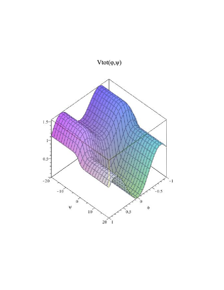
Figure 1: The potential vs the field $\varphi,\psi$ for solution 1

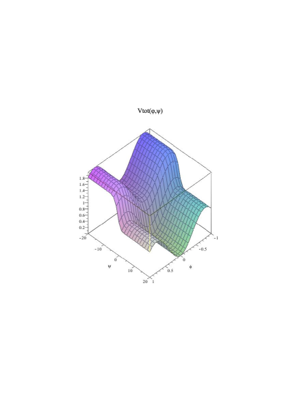
Figure 2: The potential vs the fields $\varphi,\psi$ for solution 2

The evolution of the kinetic energy for the solutions is presented in Fig. 3 and Fig. 4. The kinetic energy for the first solution (Fig. 3) is

$$K(\varphi)=\frac{1}{\kappa}\left[-\frac{m\alpha^{2}}{4}\sin^{2}(2\tilde{\varphi})+\epsilon\frac{(\cos(\tilde{\varphi}))^{4m}}{a_{i}^{2}}\right].$$ (41)

We note the local maximum at an inflationary period ($t\sim 0$). The kinetic energy for the second solution (Fig. 4)

$$K(\varphi,\psi)=\frac{1}{\kappa}\left[-\frac{m\alpha^{2}}{4}\sin^{2}(2\tilde{\varphi})+\frac{\epsilon}{A^{2}}\left(\beta+\exp{\alpha\left(\sqrt{\frac{\kappa}{2\epsilon}}(\psi-\psi_{0})\right)}\right)^{-2m}\right],$$ (42)

has a local maximum in respect of the phantom field $\varphi$ during the inflationary period.

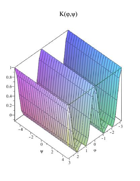
Figure 3: The kinetic energy vs the field $\varphi$ for solution 1

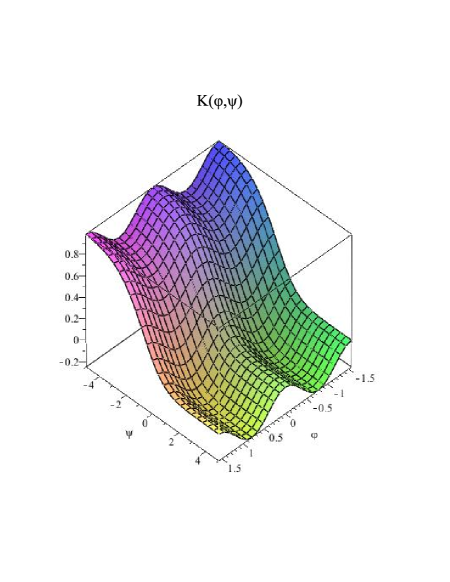
Figure 4: The kinetic energy vs the fields $\varphi,\psi$ for solution 2

5 Key cosmological parameters of EmU

We have obtained two classes of exact solutions and therefore it is possible to apply the method of calculation of the cosmological parameters for this case [7]. We calculate the parameters in accordance with the general approach at the time when the perturbation with wave vector $\vec{k}$ is crossing the horizon: $aH=k$. Let us denote by $t_{*}$ the time of horizon crossing. Then the results for scalar type perturbations is presented by a power spectrum of the form

$$P_{R}(k)=\frac{m^{3}\alpha^{2}e^{3\alpha t_{*}}}{8M_{p}^{2}\beta(\beta+e^{\alpha t_{*}})^{2}},$$ (43)

and by spectral index

$$n_{S}(k)-1=\frac{3\beta+e^{\alpha t_{*}}}{me^{\alpha t_{*}}+\beta}.$$ (44)

The power spectrum for tensor perturbations (gravitational waves) is

$$P_{G}(k)=\frac{m^{2}\alpha^{2}e^{2\alpha t_{*}}}{2M_{p}^{2}(\beta+e^{\alpha t_{*}})^{2}}.$$ (45)

The spectral index for tensor perturbations is

$$n_{G}=\frac{2\beta}{me^{\alpha t_{*}}+\beta}.$$ (46)

Also we can calculate the tensor to scalar ratio (T/S ratio) as

$$\frac{T}{S}=4\frac{\beta}{me^{\alpha t_{*}}}.$$ (47)

In the formulas above, $t_{*}$ is the time of horizon crossing. These formulas can be used to make some restrictions for the EmU parameters by comparing cosmological parameters with observational data. But this procedure lies outside the framework of this article and is a topic for future work.

6 Discussion

An EmU scenario is of great interest because of the possibility of avoiding the initial singularity and a quantum gravity era. Various aspects of the EmU scenario have been discussed in the literature (see, e.g., [3]). In the present article, we have continued our investigations connected with the consideration of a NSM as the source of the EmU started in the work [4]. There, a two-component NSM was presented as the source supporting the EmU development in time. The study was performed for special regimes: early times ($t\rightarrow-\infty$) and inflationary expansion. There were found solutions especially for these regimes.

As the next step of the investigation, we studied [3] the two-component CCM without any restriction to special regimes; the entire evolution of the EmU was analyzed. a few asymptotic solutions were found and some facts about the kinetic interaction between dark sector fields were obtained via an analysis of the chiral metric components $h_{22}$ (which is responsible for the kinetic interaction in that model). An example of an exact solution was found also which gave us hope to describe a global evolution of the EmU from $t\rightarrow-\infty$ to the infinite future and to calculate the cosmological parameters for comparison with observational data.

In the present letter we report two new classes of exact solutions which are valid for the entire evolution of the Universe. The general features of the obtained solutions provide a strong indication that two types of scalar fields are needed: one field should be of the phantom type while the other should be a canonical one. Thus we arrive at a generalization of the quintom model [8] and with the arguments above, we suggest that this model be called a phantonical EmU. Therefore only such a distribution between the fields will protect the EmU from decay and give us the possibility to have global evolution.

By analyzing the total potentials for both solutions (Fig. 1 and Fig. 2), we find an analogy with the potential for hybrid inflation [9]. But if we will follow some regime with say $\psi=constant$, the result will show a decay of the scale factor from the EmU one (7).

Let us also pay attention to the presently observed accelerated expansion of the Universe. In the framework of the scale factor (7), we could not model an accelerated expansion. Therefore we may suggest the decay of the EmU with dark energy domination during the recent history of the Universe. It will be possible to use the approach suggested in [10], viz., to consider a chiral cosmological model coupled to a perfect fluid with the aim of considering cold dark matter.

We would like to stress once again that with the exact solutions of the EmU, there is the possibility of calculating the cosmological parameters [7] without attracting a slow roll approximation which is often used for this purpose. We presented the results of a such a calculation and in future, we hope to obtain limitations for the EmU model parameters from observational data.

7 Acknowledgments

SVC is thankful to the University of KwaZulu-Natal, the University of Zululand and the NRF for financial support and warm hospitality during his visit in 2012 to South Africa. SDM acknowledges that this work is based upon research supported by the South African Research Chair Initiative of the Department of Science and Technology and the National Research Foundation.

References

- [1] G.R.F. Ellis, R. Maartens, Class. Quantum Grav. 21 (2002) 223-232.
- [2] G.R.F. Ellis, J. Murgan, C. Tsagas, Class. Quantum Grav. 21 (2004) 233-250.
- [3] A. Beesham, S.V. Chervon, S.D. Maharaj, A.S. Kubasov, Quantum Matter (ISSN: 2164-7615), v.2, (2013) 388-395.
- [4] A. Beesham, S.V. Chervon, S.D. Maharaj, Class. Quantum Grav. 26 (2009) 075017.
- [5] S.V. Chervon, V.M. Zhuravlev, V.K. Shchigolev, Phys. Lett. B 398 (1997) 269.
- [6] S. Mukherjee, B.C. Paul, N.K. Dadhich, S.D. Maharaj, A. Beesham, Class. Quantum Grav., 23 (2006) 6927.
- [7] S.V. Chervon, I.V. Fomin, Gravitation & Cosmology, 14 (2008) 163-167.
- [8] S.V. Chervon, Quantum Matter (ISSN: 2164-7615), v.2, (2013) 72-83.
- [9] A. Linde, Phys. Rev. D49(1994) 748-754.
- [10] R.R. Abbyazov, S.V. Chervon, Gravitation & Cosmology, 18 (2012) 262-269.