High-Order Coupled Cluster Method Calculations using Three-Dimensional Model States: An Illustration for the Triangular-Lattice Antiferromagnet in an External Field

Abstract

The coupled cluster method (CCM) has previously been applied to study the ground- and excited-state properties of many different types of frustrated and unfrustrated quantum spin systems. A common feature in the application of the CCM is to rotate the local spin axes of the (often classical) model state so that (notationally only) the spins all appear to point in the downwards $z$-direction. Hitherto, we remark that only coplanar model states have been used because they do not lead to imaginary terms in the new Hamiltonian. By contrast, non-coplanar “three-dimensional” (3D) model states can lead to imaginary terms in the new Hamiltonian after rotation. In principle, however, macroscopic quantities predicted by the CCM (such as the ground-state energy and order parameter) should still be real (even though the Hamiltonian may be complex) because the transformations of local spin axes are unitary. Here we explain how we may use such 3D model states for the CCM and how we may solve for the (now possibly complex) CCM correlation coefficients. We present results for the spin-half triangular-lattice antiferromagnet in an external magnetic field. We use both coplanar model states and a single 3D non-coplanar model state. We calculate the ground-state energy and the lattice magnetization as a function of the magnetic field strength. We find that the energies of the coplanar states lie lower than that of the non-coplanar state for all values of the external field, as seen in other approximate studies for this model. We find that the non-coplanar state does not detect the well-known spin plateau occurring in this model, although (as seen before) it is clearly observed for the coplanar model states using the CCM. These results are an excellent initial validation of the new approach for the application of the CCM using 3D model states.

I Introduction

In this article we apply a method of quantum many-body theory called the coupled cluster method (CCM) ccm1 ; ccm2 ; ccm5 ; ccm12 ; ccm15 ; ccm20 ; ccm26 ; ccm27 ; ccm32 ; ccm35 to study strongly interacting quantum spin systems. The CCM is not restricted, in principle, by the spatial dimensionality of the problem or by the presence of competition between bonds, i.e., in frustrated quantum spin systems. An important advance in the accuracy of the method for a localized approximation scheme called the LSUB$m$ scheme has been afforded by the use of “high-order” CCM via computer-algebraic implementations ccm12 ; ccm15 ; ccm20 ; ccm26 . This computer code developed by DJJ Farnell and J Schulenburg code is very flexible in terms of the range of underlying crystallographic lattices, values for spin quantum number, and types of Hamiltonian that may be studied. A common first task in the practical application of the CCM is to rotate the local spin axes of the (often classical) model state so that (notationally only) the spins all appear to point in the downwards $z$-direction. Although the Hamiltonian is changed by transforming these local spin axes, these rotations are unitary and so they do not affect the energy eigenvalues or expectation values. Furthermore, we note that hitherto only coplanar model states have been used because they do not lead to complex numbers in the new Hamiltonian. By contrast, three dimensional (3D) non-coplanar model states can lead to imaginary terms in the new Hamiltonian after rotation and so are more difficult to treat computationally. In principle, however, macroscopic quantities predicted by the CCM (such as the ground-state energy and order parameter) should be still real even though the Hamiltonian is now complex because again these transformations of local spin axes are unitary. Here we explain how we may use such 3D model states for the CCM and how we may solve for the (now possibly complex) CCM correlation coefficients.

As an illustration of the method, we consider the spin-half triangular-lattice Heisenberg antiferromagnet in a magnetic field LhuiMi ; hon1999 ; CGHP ; squareTriangleED ; HSR04 . As is well-known, the response of quantum magnetic systems to an external field is revealed by its magnetization curve. The magnetic processes of quantum anitferromagnets is discussed, e.g., in Refs. hon1999 ; squareTriangleED ; HSR04 ; nishi ; chub ; alicea ; oshi ; SchuRi ; jump ; ono ; kagome_pl ; schnalle ; schroeder ; fortune , and the interested reader is referred to these sources for more details. The Hamiltonian that we will use here is given by

$$H=\sum_{\langle i,j\rangle}{\bf s}_{i}~{}\cdot~{}{\bf s}_{j}-\lambda\sum_{i}s_{i}^{z}~{}~{},$$ (1)

where the index $i$ runs over all lattice sites on the triangular lattice. The expression $\langle i,j\rangle$ indicates a sum over all nearest-neighbor pairs, although each pair is counted once and once only. The strength of the applied external magnetic field is given by $\lambda$.

There are two ground states classically (shown in Fig. 1): a set of coplanar states and a single non-coplanar state. The quantum system is discussed in Refs. hon1999 ; HSR04 ; nishi ; chub ; alicea ; chub94 ; trumper00 ; ono ; squareTriangleED . Although on the classical level both cases (coplanar and non-coplanar) are energetically equivalentkawamura ; chub ; zhito ; cabra , previous results of approximate methods indicate that thermal or quantum fluctuations ought to favor the planar configuration kawamura ; chub ; zhito ; cabra . Previous results of the CCM farnell indicate that a plateau state occurs for $1.37\lesssim\lambda\lesssim 2.15$. (Note that we compare new results presented in this article for the non-coplanar states to those earlier results of Ref. farnell .) These results for the plateau are in excellent agreement with experimental results for the magnetic compound Ba₃CoSb₂O₉ (a spin-half triangular-lattice antiferromagnet), which demonstrates a spin plateau that agrees quantitatively with results of the CCM and exact diagonalizations shirata . Furthermore, CCM results indicate that a similar plateau occurs over the range $2.82\lesssim\lambda\lesssim 3.70$ for the for the spin-one triangular-lattice antiferromagnet, and this theoretical result has subsequently been established experiment for the compound Ba₃NiSb₂O₉ (a spin-one triangular-lattice antiferromagnet) richter .

The main goal of our paper is to explain how the CCM can be used with 3D model states. Firstly we present a brief description of the CCM formalism and its application via computational methods to the subject of quantum spin models with 3D model states. As an illustration of our method, we describe the application of the method to the spin-half Heisenberg model for the triangular lattice at zero temperature in the presence of an external magnetic field. We present our results and then discuss the conclusions of this research.

II The Coupled Cluster Method (CCM)

As the CCM has been discussed extensively elsewhere (see Refs. ccm1 ; ccm2 ; ccm5 ; ccm12 ; ccm15 ; ccm20 ; ccm26 ; ccm27 ; ccm32 ; ccm35 ), a brief overview of the method is presented here only. Note however that the solution of the CCM equations for the case of 3D model states is presented in an Appendix, which has not been attempted before. In this case, CCM correlation coefficients may be complex, and so extensive changes to the basic computer code that implements the CCM to high orders of approximation are necessary, again as described in the Appendix. We begin the brief overview of the CCM method by presenting the ground-state Schrödinger equations, which are given by

$$H|\Psi\rangle=E_{g}|\Psi\rangle\;;\;\;\;\langle\tilde{\Psi}|H=E_{g}\langle\tilde{\Psi}|\;.$$ (2)

and bra and ket states are given by

$$|\Psi\rangle={\rm e}^{S}|\Phi\rangle\; \;\;\;S=\sum_{I\neq 0}{\cal S}_{I}C_{I}^{+}\;,$$ ;

$$\langle\tilde{\Psi}|=\langle\Phi|\tilde{S}{\rm e}^{-S}\; \;\;\;\tilde{S}=1+\sum_{I\neq 0}\tilde{{\cal S}}_{I}C_{I}^{-}\;.$$ ; (3)

We use model states (denoted $|\Phi\rangle$ in the ket state and $\langle\Phi|$ in the bra state) as references states for the CCM and those used here are shown in Fig. 1.

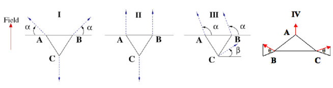
Figure 1: Classical ground states (also the CCM model states): I to III are coplanar, whereas IV is non-coplanar with spins at an angle $\theta$ to the plane perpendicular to the external field.

We note that the CCM ket- and bra-state equations are given by

$$\langle\Phi|C_{I}^{-}{\rm e}^{-S}H{\rm e}^{S}|\Phi\rangle = 0,\;\;\forall I\neq 0\;\;;$$ (4)

$$\langle\Phi|\tilde{S}{\rm e}^{-S}[H,C_{I}^{+}]{\rm e}^{S}|\Phi\rangle = 0,\;\;\forall I\neq 0\;\;.$$ (5)

and that the method in which Eqs. (4) and (5) are solved has been discussed extensively elsewhere ccm1 ; ccm2 ; ccm5 ; ccm12 ; ccm15 ; ccm20 ; ccm26 ; ccm27 ; ccm32 ; ccm35 and so is not given here. The ground-state energy is given by

$$E_{g}=\langle\Phi|e^{-S}He^{S}|\Phi\rangle~{}~{}.$$ (6)

This equation is a function of the ket-state correlation coefficients only.

We differentiate between those the model states that are coplanar and the single model state that is non-coplanar (or “3D”). The analysis for the coplanar model state is given in Ref. farnell and we refer the interested reader to this publication for more details. The non-coplanar model state IV has spins that make an angle $\theta$ to the plane perpendicular to the external field, as is also shown in Fig. 1. We rotate the local spin axes of the spins such that all spins appear to point downwards for all four model states I, II, III, and IV in Fig. 1.

We have four new Hamiltonians after rotation of the local spin axes of the spins such that all spins appear to point downwards for all four model states I, II, III, and IV in Fig. 1(a-d).

The Hamiltonian for model state I, Fig. 1 after rotation of the local spin axes is given by:

$$H = \sum_{\langle i_{A}\rightarrow i_{B}\rangle}\biggl{\{}-\frac{1}{4}(1+{\rm cos}(2\alpha))(s_{i_{A}}^{+}s_{i_{B}}^{+}+s_{i_{A}}^{-}s_{i_{B}}^{-})$$ (7)

$$~{}~{}~{}~{}~{}~{}~{}+\frac{1}{4}(1-{\rm cos}(2\alpha))(s_{i_{A}}^{+}s_{i_{B}}^{-}+s_{i_{A}}^{-}s_{i_{B}}^{+})$$

$$~{}~{}~{}~{}~{}~{}~{}-{\rm cos}(2\alpha)s_{i_{A}}^{z}s_{i_{B}}^{z}+\frac{1}{2}{\rm sin}(2\alpha)(s_{i_{A}}^{z}s_{i_{B}}^{+}+s_{i_{A}}^{z}s_{i_{B}}^{-})$$

$$~{}~{}~{}~{}~{}~{}~{}-\frac{1}{2}{\rm sin}(2\alpha)(s_{i_{A}}^{+}s_{i_{B}}^{z}+s_{i_{A}}^{-}s_{i_{B}}^{z})\biggr{\}}$$

$$+ \sum_{\langle i_{B,C}\rightarrow i_{C,A}\rangle}\biggl{\{}-\frac{1}{4}(1+{\rm sin}(\alpha))(s_{i_{B,C}}^{+}s_{i_{C,A}}^{+}+s_{i_{B,C}}^{-}s_{i_{C,A}}^{-})$$

$$~{}~{}~{}~{}~{}~{}~{}+\frac{1}{4}(1-{\rm sin}(\alpha))(s_{i_{B,C}}^{+}s_{i_{C,A}}^{-}+s_{i_{B,C}}^{-}s_{i_{C,A}}^{+})$$

$$~{}~{}~{}~{}~{}~{}~{}-{\rm sin}(\alpha)s_{i_{B,C}}^{z}s_{i_{C,A}}^{z}+\frac{1}{2}{\rm cos}(\alpha)(s_{i_{B,C}}^{z}s_{i_{C,A}}^{+}+s_{i_{B,C}}^{z}s_{i_{C,A}}^{-})$$

$$~{}~{}~{}~{}~{}~{}~{}-\frac{1}{2}{\rm cos}(\alpha)(s_{i_{B,C}}^{+}s_{i_{C,A}}^{z}+s_{i_{B,C}}^{-}s_{i_{C,A}}^{z})\biggr{\}}$$

$$- \lambda\sum_{i_{C}}s_{i_{C}}^{z}+\lambda{\rm sin}(\alpha)\left(\sum_{i_{A}}s_{i_{A}}^{z}+\sum_{i_{B}}s_{i_{B}}^{z}\right)$$

$$- \frac{\lambda}{2}{\rm cos}(\alpha)\sum_{i_{A}}(s_{i_{A}}^{+}+s_{i_{A}}^{-})+\frac{\lambda}{2}{\rm cos}(\alpha)\sum_{i_{B}}(s_{i_{B}}^{+}+s_{i_{B}}^{-})\;,$$

where the sum $\langle i_{A}\rightarrow i_{B}\rangle$ goes from sublattice $A$ to sublattice $B$ (and with directionality). Note that $\langle i_{B,C}\rightarrow i_{C,A}\rangle$ indicates a sum that goes from sublattice $B$ to sublattice $C$ and sublattice $C$ to sublattice $A$, respectively (and with directionality).

The Hamiltonian for model state III, Fig. 1 after rotation of the local spin axes is given by:

$$H = \sum_{\langle i_{C}\rightarrow i_{A,B}\rangle}\biggl{\{}\frac{1}{4}(-1+{\rm cos}(\alpha-\beta))(s_{{i_{C}}}^{+}s_{{i_{A,B}}}^{+}+s_{{i_{C}}}^{-}s_{{i_{A,B}}}^{-})$$ (8)

$$~{}~{}~{}~{}~{}~{}~{}+\frac{1}{4}(1+{\rm cos}(\alpha-\beta))(s_{{i_{C}}}^{+}s_{{i_{A,B}}}^{-}+s_{{i_{C}}}^{-}s_{{i_{A,B}}}^{+})$$

$$~{}~{}~{}~{}~{}~{}~{}+{\rm cos}(\alpha-\beta)s_{{i_{C}}}^{z}s_{{i_{A,B}}}^{z}$$

$$~{}~{}~{}~{}~{}~{}~{}+\frac{1}{2}{\rm sin}(\alpha-\beta)(s_{{i_{C}}}^{+}s_{{i_{A,B}}}^{z}+s_{{i_{C}}}^{-}s_{{i_{A,B}}}^{z})$$

$$~{}~{}~{}~{}~{}~{}~{}-\frac{1}{2}{\rm sin}(\alpha-\beta)(s_{{i_{C}}}^{z}s_{{i_{A,B}}}^{+}+s_{{i_{C}}}^{z}s_{{i_{A,B}}}^{-})\biggr{\}}$$

$$+ \sum_{\langle i_{A},i_{B}\rangle}\biggl{\{}\frac{1}{2}(s_{i_{A}}^{+}s_{i_{B}}^{-}+s_{i_{A}}^{-}s_{i_{B}}^{+})+s_{i_{A}}^{z}s_{i_{B}}^{z}\biggr{\}}$$

$$+ \lambda{\rm sin}(\alpha)\left(\sum_{i_{A}}s_{i_{A}}^{z}+\sum_{i_{B}}s_{i_{B}}^{z}\right)+\lambda{\rm sin}(\beta)\sum_{i_{C}}s_{i_{C}}^{z}$$

$$+ \frac{\lambda}{2}{\rm cos}(\alpha)\left\{\sum_{i_{A}}(s_{i_{A}}^{+}+s_{i_{A}}^{-})+\sum_{i_{B}}(s_{i_{B}}^{+}+s_{i_{B}}^{-})\right\}$$

$$+ \frac{\lambda}{2}{\rm cos}(\beta)\sum_{i_{C}}(s_{i_{C}}^{+}+s_{i_{C}}^{-})\;,$$

where the sum $\langle i_{C}\rightarrow i_{A,B}\rangle$ goes from sublattice $C$ to sublattices $A$ and $B$ (with directionality) and $\langle i_{A},i_{B}\rangle$ goes over each bond connecting the $A$ and $B$ sublattices, but counting each one once only (and without directionality). We note that we have three sites in the unit cell for all of the models states used for the triangular lattice antiferromagnet. The Hamiltonian for model state II, Fig. 1, is a limiting case of Eqs. (7) and (8).

The Hamiltonian for the non-coplanar model state IV after rotation of the local spin axes is given by:

$$H = \sum_{\langle i\rightarrow j\rangle}\biggl{\{}(\sin^{2}(\theta)-\frac{1}{2}\cos^{2}(\theta))s_{i}^{z}s_{j}^{z}$$ (9)

$$~{}~{}~{}~{}~{}~{}~{}+\frac{1}{4}\left(\frac{1}{2}\sin^{2}(\theta)-\cos^{2}(\theta)-\frac{1}{2}\right)(s_{i}^{+}s_{j}^{+}+s_{i}^{-}s_{j}^{-})$$

$$~{}~{}~{}~{}~{}~{}~{}+\frac{1}{4}\left(\cos^{2}(\theta)-\frac{1}{2}\sin^{2}(\theta)-\frac{1}{2}\right)(s_{i}^{+}s_{j}^{-}+s_{i}^{-}s_{j}^{+})$$

$$~{}~{}~{}~{}~{}~{}~{}+\frac{\sqrt{3}}{4}{\rm cos}(\theta)\big{(}s_{i}^{z}\{s_{j}^{+}+s_{j}^{-}\}-\{s_{i}^{+}+s_{i}^{-}\}s_{j}^{z}\big{)}\biggr{\}}$$

$$+ \lambda\sum_{i}{\rm sin}(\theta)s_{i}^{z}$$

$$+ {\rm i}\sum_{\langle i\rightarrow j\rangle}\biggl{\{}\frac{\sqrt{3}}{4}{\rm sin}(\theta)(s_{i}^{+}s_{j}^{-}-s_{i}^{-}s_{j}^{+})$$

$$~{}~{}~{}~{}~{}~{}~{}+\frac{3}{4}{\rm sin}(\theta){\rm cos}(\theta)\big{(}s_{i}^{z}\{s_{j}^{+}-s_{j}^{-}\}+\{s_{i}^{+}-s_{i}^{-}\}s_{j}^{z}\big{)}\biggr{\}}$$

$$+ {\rm i}\frac{\lambda}{2}\sum_{i}{\rm cos}(\theta)(s_{i}^{+}-s_{j}^{-})\;,$$

where $\langle i\rightarrow j\rangle$ are those “directional” nearest-neighbor bonds on the triangular going from the $A$ sublattice to $B$ sublattice, $B$ sublattice to $C$ sublattice, and $C$ sublattice to $A$ sublattice (in those directions only and not reversed). We see that this Hamiltonian now contains “real and imaginary components”. Henceforth, we shall take the expression “real and imaginary components” to mean that the rotated Hamiltonian contains explicit factors involving the imaginary number $i\equiv\sqrt{(}-1)$ and other explicit factors that do not involve this imaginary number. We note that $\theta$ is the angle that the spins make to the plane perpendicular to the applied external field. Full details of the rotations used in the derivation of this Hamiltonian are presented in Appendix B.

The manner in which CCM equations may be solved for the bra- and ket-state equations when correlation coefficients are allowed to be complex is discussed in the Appendix, although we note that the problem essentially reduces to a doubling of the number of CCM equations to be solved (i.e., for the real and imaginary components separately). However, we note that we use the LSUB$m$ approximation (in which clusters of $m$ contiguous sites limited to $m$ spin flips are included in $S$ and $\tilde{S}$) and that we consider the angles as free parameters in the CCM calculation. These angles are found by direct minimization of the CCM ground-state energy. This was achieved computationally at a given level of LSUB$m$ approximation, and a minimum ground state energy with respect to these canting angles was also found computationally for a given fixed value of $\lambda$. We note that there was only one angle was needed for model states I and IV, whereas two such angles were needed for model state III. Values of $\lambda$ were varied incrementally and the minimization process of the energy with respect to the canting angles repeated. The CCM calculations are costly in terms of computing time because we needed to minimize the ground-state energy with respect to such angles at each value of $\lambda$. We remark that the we have twice as many equations to solve for the 3D model state (for the real and imaginary components separately) “as normal” for the CCM. For this reason, results up to the LSUB6 level of approximation only are quoted in these initial tests, although we find that ground-state energies are highly converged for all model states even at this relatively low level of approximation.

In order to investigate the magnetization process in antiferromagnets, we consider the total lattice magnetization $M$ along the direction of the magnetic field. We note that the important Hellmann-Feynman theorem is obeyed by the CCM and so we may obtain the lattice magnetization by finding $M=-\partial(E_{g}/N)/\partial\lambda$, which is carried out computationally in this paper. The method by which other expected values may be found is also discussed in the Appendix.

III Results

As mentioned above, we present CCM results for model states I, II, III, and IV shown in Fig. 1. The computational effort of the CCM calculations presented here for the non-coplanar model state IV to very high orders is very great and so results up to LSUB6 are presented here only for this model state in these initial studies. Results of the coplanar model states I to III from Ref. farnell up to LSUB6 are also presented here for the purposes of comparison only, although we note that higher orders of approximation than LSUB6 were carried out in Ref. farnell for these states.

The results for the ground-state energy are shown in Fig. 2. We note that the results for the coplanar model states I to III from Ref. farnell with lowest energy are shown only as a function of $\lambda$ in Fig. 2. Thus, results of model state I only are presented for small values of the applied magnetic field strength $\lambda$ and results of model state III only are presented for higher values of $\lambda$ near to $\lambda_{s}$. The results of both model states coincide in the intermediate regime. Again, these LSUB$m$ series of results are found to converge rapidly with increasingly levels of LSUB$m$ approximation over all values of the external field parameter $\lambda$.

Results for model state IV are also shown. Firstly, we note that the imaginary component of the ground-state energy is found to sum to zero, as expected and required. Furthermore, the results for the ground-state energies for model state IV are much higher in value than their coplanar counterparts at identical levels of LSUB$m$ approximation. Note that LSUB6 was the highest level of approximation possible for this model state in these initial tests and so we limit all presented results (for all model states) to this level of approximation in order to allow a direct and unbiased comparison. However, we see that results for the ground-state energy are highly converged even at the LSUB6 level of approximation (by comparing results of LSUB6 to LSUB5 and LSUB4 in Fig. 2) and so these results are adequate to establish that the ground-state energies are indeed lower for the coplanar case. As noticed previously kawamura ; chub ; zhito ; cabra , these results provide clear and strong evidence that the ground state of this system is coplanar. This case has therefore been an excellent first test of new CCM based on a non-coplanar “three-dimensional” model state.

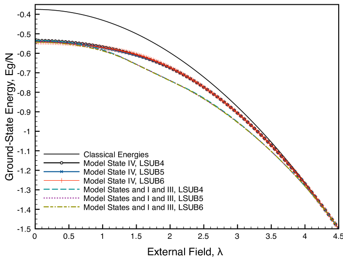
Figure 2: The ground-state energy per site, $E_{g}/N$. Energies for the coplanar states I-III from Ref. farnell are lower than those of the non-coplanar state IV for all $\lambda$.

The results for the total lattice magnetization for model states I to III from Ref. farnell are shown in Fig. 3. The LSUB$m$ results are again seen to converge rapidly for increasing $m$. However, there is a radical departure from the classical straight-line behavior (i.e. $M_{\rm{Classical}}=\frac{1}{9}\lambda$) in this case. These previous CCM results for the coplanar states accurately detect the plateau in the $M$ versus $\lambda$ curve at $M=\frac{1}{6}$. Indeed, these previous results of the CCM farnell for the coplanar model states carried out to the LSUB8 level of approximation indicate that the width of this plateau is given by $1.37\lesssim\lambda\lesssim 2.15$. (Note that the plateau corresponds to the “straight” part of the curve in the $E_{g}(\lambda)$ curve shown in Fig. 2.)

By contrast, we note that the new results from model state IV show no such spin plateau any level of LSUB$m$ attempted (e.g., LSUB4, LSUB5 and LSUB6 shown in the Fig. 3). Note that this plateau has been observed for this system by other approximate methods and in experiment shirata . We note importantly again that the lattice magnetization must be real-valued because we find values for this quantity by taking first derivative of the ground-state energy, which itself is found to be real-valued (and not complex) for all values of $\lambda$. All of these results are excellent corroborating evidence that the ground state is not of the type shown by model state IV (i.e., non-coplanar), but is rather of coplanar type shown by model states I to III. Again, this is an excellent first check of the method for 3D model states.

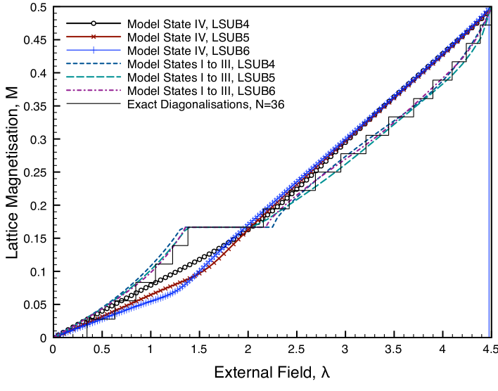
Figure 3: The lattice magnetization, $M$. Results for model state IV do not detect the spin plateau at $M=1/6$.

IV Conclusions

In this article we described how the coupled cluster method (CCM) may be applied to study the behavior of quantum magnets with the aid of non-coplanar “3D” model states. A (slightly) modified method for solving for the CCM equation by “direct iteration” and for complex CCM correlation coefficients is presented in an Appendix. We employed new computer code to find the ground-state energy and the total lattice magnetization of the spin-half triangular-lattice antiferromagnetic systems in the presence of external magnetic fields for both coplanar and non-coplanar model states (which are the classical ground states). It was found that the ground-state energy was real-valued for the non-coplanar model state, as expected and required. Results up to LSUB6 were possible only in these initial tests for the non-coplanar model state due to the increased computational complexity of the problem. However, these results were clearly highly converged even at this level of approximation. In agreement with previous results of other methods, the coplanar states were found to have lower energy. Furthermore, the spin plateau for $M=\frac{1}{6}$ known to occur in this system was detected by the coplanar model states, although it was not detected by the non-coplanar model state at any level of approximation. We conclude that the spin-half triangular lattice antiferromagnet in an external magnetic field for the non-coplanar model state has been an excellent first test of new CCM based for a non-coplanar “three-dimensional” model state.

Appendix A Using 3D Model States For the CCM

The method by which 3D model states may be employed for the high-order CCM code is discussed below. The results for the application of this new approach to the spin-half triangular lattice antiferromagnet in an external magnetic field are presented in the main text.

A.1 Ket-State Equations

Normally we solve the CCM equations either by using Newton-Raphson method or by directly iterating the CCM equations. The direct iteration method for the ket-state is achieved by casting the $N_{f}$ basic CCM equations (each corresponding to one of the $N_{f}$ fundamental clusters at a given level of approximation), namely:

$$\langle\Phi|C_{I}^{-}{\rm e}^{-S}H{\rm e}^{S}|\Phi\rangle=f_{I}=0~{}~{},$$ (10)

which we write as

$$f_{I}({\rm consts.},x_{1},\cdots,x_{N_{f}},x_{1}^{2},\cdots,x_{N_{f}}^{2},x_{1}^{3},\cdots,x_{N_{f}}^{4},x_{1}^{4},\cdots,x_{N_{f}}^{4})=0~{}~{}.$$ (11)

We then rearrange this equation into the form

$$\alpha_{l}\times x_{l}=f_{I}^{\prime}({\rm consts.},x_{1},\cdots,x_{l-1},x_{l+1},\cdots,x_{N_{f}},x_{1}^{2},\cdots,x_{N_{f}}^{2},x_{1}^{3},\cdots,x_{N_{f}}^{4},x_{1}^{4},\cdots,x_{N_{f}}^{4})~{}~{}.$$ (12)

Hence, given an initial starting solution for the set of correlation coefficients $\{x_{1},\cdots,x_{N_{f}}\}$, we iterate the following equation for all of the $N_{f}$ equations to convergence:

$$x_{l}=\frac{f_{I}^{\prime}({\rm consts.},x_{1},\cdots,x_{l-1},x_{l+1},\cdots,x_{N_{f}},x_{1}^{2},\cdots,x_{N_{f}}^{2},x_{1}^{3},\cdots,x_{N_{f}}^{4},x_{1}^{4},\cdots,x_{N_{f}}^{4})}{\alpha_{l}}~{}~{}.$$ (13)

This simple approach is successful in solving the CCM equations when all of the correlation coefficients are real.

However, for 3D model states we cannot ensure that the Hamiltonian is real-valued after rotation of the local spin axes. Indeed, in most cases it will not be so. The extension of the direct-iteration approach to complex solutions for the CCM ket-state correlation coefficients might be achieved computationally by using complex data type (and all operators) using C++ classes. However, the changes to the CCM code would be extensive. A simpler alternative is just to break the $N_{f}$ CCM equations to $2\times N_{f}$ equations, corresponding to the real and complex parts of the equation(s) governed by Eq. (12).

Hence, we split $x_{l}$ into real and imaginary components, i.e., $x_{l}=a_{l}+{\rm i}b_{l}$, as well as $\alpha_{l}=\beta_{l}+{\rm i}\gamma_{l}$ and $f_{l}^{\prime}=g_{l}+{\rm i}h_{l}$ such that

$$a_{l} = \frac{g_{I}({\rm consts.},x_{1},\cdots,x_{l-1},x_{l+1},\cdots,x_{N_{f}},x_{1}^{2},\cdots,x_{N_{f}}^{2},x_{1}^{3},\cdots,x_{N_{f}}^{4},x_{1}^{4},\cdots,x_{N_{f}}^{4})+\gamma_{l}b_{l}}{\beta_{l}}$$

$$b_{l} = \frac{h_{I}({\rm consts.},x_{1},\cdots,x_{l-1},x_{l+1},\cdots,x_{N_{f}},x_{1}^{2},\cdots,x_{N_{f}}^{2},x_{1}^{3},\cdots,x_{N_{f}}^{4},x_{1}^{4},\cdots,x_{N_{f}}^{4})-\alpha_{l}a_{l}}{\gamma_{l}}$$

We now iterate these (now) $2\times N_{f}$ equations for $a_{l}$ and $b_{l}$ (which correspond to the real and imaginary parts of ket-state correlation coefficient $x_{l}$) to convergence. Note that we use the following products identities (up to fourth order) in the CCM equations of Eq. (LABEL:directItImag), namely:

$$x_{1} = a_{1}+{\rm i}b_{1}$$

$$x_{1}\times x_{2} = (a_{1}+{\rm i}b_{1})\times(a_{2}+{\rm i}b_{2})=a_{1}a_{2}-b_{1}b_{2}+{\rm i}(a_{1}b_{2}+b_{1}a_{2})$$

$$x_{1}\times x_{2}\times x_{3} = x_{1}\times x_{2}\times(a_{3}+{\rm i}b_{3})$$

$$= a_{1}a_{2}a_{3}-b_{1}b_{2}a_{3}-b_{1}a_{2}b_{3}-a_{1}b_{2}b_{3}$$

$$+{\rm i}(b_{1}a_{2}a_{3}+a_{1}b_{2}a_{3}+a_{1}a_{2}b_{3}-b_{1}b_{2}b_{3})$$

$$x_{1}\times x_{2}\times x_{3}\times x_{4} = x_{1}\times x_{2}\times x_{3}\times(a_{4}+{\rm i}b_{4})$$

$$= a_{1}a_{2}a_{3}a_{4}-b_{1}b_{2}a_{3}a_{4}-a_{1}b_{2}b_{3}a_{4}-b_{1}a_{2}b_{3}a_{4}$$

$$-a_{1}b_{2}a_{3}b_{4}-b_{1}a_{2}a_{3}b_{4}-a_{1}a_{2}b_{3}b_{4}+b_{1}b_{2}b_{3}b_{4}$$

$$+{\rm i}(b_{1}a_{2}a_{3}a_{4}+a_{1}b_{2}a_{3}a_{4}+a_{1}a_{2}b_{3}a_{4}+a_{1}a_{2}a_{3}b_{4}$$

$$-a_{1}b_{2}b_{3}b_{4}-b_{1}a_{2}b_{3}b_{4}-b_{1}b_{2}a_{3}b_{4}-b_{1}b_{2}b_{3}a_{4})$$

These identities have been coded directly into the high-order CCM code in order to solve for complex ket-state coefficients; although this is somewhat tedious, it has the advantage of being more straightforward and probably a little speedier at runtime than using complex number classes to solve this problem.

A.2 Ground-State Energies

Ground-state energies are found by evaluating

$$E_{g}=\langle\Phi|e^{-S}He^{S}|\Phi\rangle~{}~{}.$$ (15)

We note that the ground-state energy $E_{g}$ is a function of the CCM coefficients up to quadratic terms in these coefficients (i.e., terms such as const., $x_{1}$ and $x_{1}\times x_{2}$). Hence, we use the above equations in order to find the real and imaginary parts of such terms. Furthermore, as the Hamiltonian has both real and imaginary parts we divide the ground-state energies via:

$$E_{g}=E_{g}({\rm real})+{\rm i}E_{g}({\rm imag.})~{}~{}.$$ (16)

After determining the real and imaginary components of the CCM ket-state correlation coefficient, we ought to find that $E_{g}({\rm imag.})=0$, as all of the terms contributing to it should cancel each other out. This is because that are real before rotation of local spin axes (and must $E_{g}$ clearly is real number) must still be real even though we are now solving for complex CCM correlation coefficients. Indeed, this constraint, i.e., $E_{g}({\rm imag.})=0$, forms an excellent check that our computer code is working correctly. This was found to be the case for model state IV employed here for the triangular-lattice Heisenberg antiferromagnet for all values of the external magnetic field strength, $\lambda$.

A.3 Bra-State Equations

We determine the bra-state correlation coefficient firstly by finding

$$\bar{H}=\langle\tilde{\Psi}|H|\Psi\rangle$$ (17)

and then by taking the partial derivative of this expression with respect to $x_{l}$. We note again that the bra-state operator is defined via $\tilde{S}=1+\sum_{I\neq 0}\tilde{{\cal S}}_{I}C_{I}^{-}$ and so we see that we obtain a linear equation

$$\frac{\partial\bar{H}}{\partial x_{l}}=\frac{\partial}{\partial x_{l}}\langle\tilde{\Phi}|(1+\sum_{I\neq 0}\tilde{{\cal S}}_{I}C_{I}^{-})e^{-S}He^{S}|\Phi\rangle=0$$ (18)

However, we note again that $E_{g}=\langle\Phi|e^{-S}He^{S}|\Phi\rangle$ and $\langle\Phi|C_{I}^{-}{\rm e}^{-S}H{\rm e}^{S}|\Phi\rangle=f_{I}$ and so we may write the above bra-state equation as

$$\frac{\partial\bar{H}}{\partial x_{l}}=\frac{\partial E_{g}}{\partial x_{l}}+\sum_{I\neq 0}\tilde{{\cal S}}_{I}\frac{\partial f_{I}}{\partial x_{l}}=0$$ (19)

This is just an equation that is linear in terms of the bra-state correlation coefficients. If we now write $\tilde{x}_{l}=\tilde{{\cal S}}_{I}$ then this equation is solving readily by putting the $\tilde{x}_{l}$ terms for the $l^{\rm th}$ bra-state equation on the left-hand side of the equation and everything else on the right-hand side. We then iterate to convergence once again. Previously, bra-state correlation coefficients were real-valued, although we cannot preclude that the bra-state coefficients are complex for 3D model states. Once again we solve this problem by iterating $2\times N_{f}$ bra-state equations, corresponding to the real and imaginary parts of the bra-state correlation coefficients. In this case, we have terms such as:

$$\tilde{x}_{1} = \tilde{a}_{1}+{\rm i}\tilde{b}_{1}$$

$$\tilde{x}_{1}\times x_{2} = (\tilde{a}_{1}+{\rm i}\tilde{b}_{1})\times(a_{2}+{\rm i}b_{2})=\tilde{a}_{1}a_{2}-\tilde{b}_{1}b_{2}+{\rm i}(\tilde{a}_{1}b_{2}+\tilde{b}_{1}a_{2})$$

$$\tilde{x}_{1}\times x_{2}\times x_{3} = \tilde{x}_{1}\times x_{2}\times(a_{3}+{\rm i}b_{3})$$

$$= \tilde{a}_{1}a_{2}a_{3}-\tilde{b}_{1}b_{2}a_{3}-\tilde{b}_{1}a_{2}b_{3}-\tilde{a}_{1}b_{2}b_{3}$$

$$+{\rm i}(\tilde{b}_{1}a_{2}a_{3}+\tilde{a}_{1}b_{2}a_{3}+\tilde{a}_{1}a_{2}b_{3}-\tilde{b}_{1}b_{2}b_{3})$$

$$\tilde{x}_{1}\times x_{2}\times x_{3}\times x_{4} = \tilde{x}_{1}\times x_{2}\times x_{3}\times(a_{4}+{\rm i}b_{4})$$

$$= \tilde{a}_{1}a_{2}a_{3}a_{4}-\tilde{b}_{1}b_{2}a_{3}a_{4}-\tilde{a}_{1}b_{2}b_{3}a_{4}-\tilde{b}_{1}a_{2}b_{3}a_{4}$$

$$-\tilde{a}_{1}b_{2}a_{3}b_{4}-\tilde{b}_{1}a_{2}a_{3}b_{4}-\tilde{a}_{1}a_{2}b_{3}b_{4}+\tilde{b}_{1}b_{2}b_{3}b_{4}$$

$$+\,\,{\rm i}(\tilde{b}_{1}a_{2}a_{3}a_{4}+\tilde{a}_{1}b_{2}a_{3}a_{4}+\tilde{a}_{1}a_{2}b_{3}a_{4}+\tilde{a}_{1}a_{2}a_{3}b_{4}$$

$$-\tilde{a}_{1}b_{2}b_{3}b_{4}-\tilde{b}_{1}a_{2}b_{3}b_{4}-\tilde{b}_{1}b_{2}a_{3}b_{4}-\tilde{b}_{1}b_{2}b_{3}a_{4})$$

A.4 Other Expectation Values

As the well-known Helmann-Feynman theorem is obeyed by the CCM, the lattice magnetization is found by taking the first derivative of the ground-state energy per spin with respect to the external field strength $\lambda$. This was achieved computationally in this article as this approach is simple and straightforward. An alternative approach (not carried out here) may also be used to find the lattice magnetization $\langle s^{z}\rangle$. We begin by rotating the local coordinates of the spin axes and we form the relevant operator $\langle s^{z}\rangle$, which may well now be complex. However, once we have solved for both the ket-and bra-state equations we should find that the imaginary part of this quantity should sum to zero, as was indeed seen for the ground-state energy.

We note that the local “sublattice” magnetization $\langle\tilde{\Psi}|s^{z}|\Psi\rangle$ (where $s^{z}$ is expressed in spin coordinates after rotation of the local spin axes) is found to be complex. This seems perplexing at first because we are finding $\langle\tilde{\Psi}|s^{z}|\Psi\rangle$, i.e., there appears to be no imaginary term inside this expectation value! However, we see that $s^{z}$ is expressed in terms of the rotated spin axes. If we were to carry out the inverse transformation (i.e., from the rotated spin axes to the original axes) then $s^{z}$ would, of course, probably become complex-valued when expressed in terms of these original spin axes. We might well now expect this new quantity to be complex-valued, and indeed this was found to be the case. Caution should therefore be exercised in attaching importance to the “sublattice magnetization” for such 3D model states, although it might be well-defined in certain circumstances. This is quite different to coplanar 2D model states for the CCM, and for which the sublattice magnetization is always real.

To summarize, however, only those macroscopic observables that are real-valued in the original spin coordinates for 3D model states ought definitely to be real-valued once we have solved for the ket- and bra-state equations and formed the relevant expectation values. In these cases, imaginary components present after rotation of local spin axes should sum to zero when evaluating the expectation value.

Appendix B Rotation of the local spin axes

We now present a derivation of the Hamiltonian after rotation of the local spin axes. We begin by again presenting the Hamiltonian before rotation of the spin axes:

$$H=\sum_{\langle i,j\rangle}{\bf s}_{i}~{}\cdot~{}{\bf s}_{j}-\lambda\sum_{i}s_{i}^{y}~{}~{},$$ (20)

where the index $i$ runs over all lattice sites on the triangular lattice. The expression $\langle i,j\rangle$ indicates a sum over all nearest-neighbor pairs, although each pair is counted once and once only. The strength of the applied external magnetic field is given by $\lambda$. Note that we assume that the external field applies now in the $y$-direction rather than the $z$-direction. This is a notational change only in order to simplify somewhat the following mathematics and it does not affect our results. Indeed, this choice allows us to use the model state with zero field now lies in the $xz$-plane, as used in Ref. ccm12 .

The classical ground-state of Eq. (20) when $\lambda=0$ is the Néel-like state where all spins on each sublattice are separately aligned (again as in Ref. ccm12 , all in the $xz$-plane, say). The spins on sublattice A are oriented along the negative z-axis, and spins on sublattices B and C are oriented at $+120^{\circ}$ and $-120^{\circ}$, respectively, with respect to the spins on sublattice A. We perform the following spin-rotation transformations. Specifically, we leave the spin axes on sublattice A unchanged, and we rotate about the $y$-axis the spin axes on sublattices B and C by $-120^{\circ}$ and $+120^{\circ}$ respectively,

$$s_{B}^{x}\rightarrow-\frac{1}{2}s_{B}^{x}-\frac{\sqrt{3}}{2}s_{B}^{z}\;\; \;\;s_{C}^{x}\rightarrow-\frac{1}{2}s_{C}^{x}+\frac{\sqrt{3}}{2}s_{C}^{z}\;\;,$$ ;

$$s_{B}^{y}\rightarrow s_{B}^{y}\;\; \;\;s_{C}^{y}\rightarrow s_{C}^{y}\;\;,$$ ;

$$s_{B}^{z}\rightarrow\frac{\sqrt{3}}{2}s_{B}^{x}-\frac{1}{2}s_{B}^{z}\;\; \;\;s_{C}^{z}\rightarrow-\frac{\sqrt{3}}{2}s_{C}^{x}-\frac{1}{2}s_{C}^{z}\;\;.$$ ; (21)

This leads to a Hamiltonian given by:

$$H=\sum_{\langle i\rightarrow j\rangle}\left\{-{1\over 2}s_{i}^{x}s_{j}^{x}+s_{i}^{y}s_{j}^{y}-{1\over 2}s_{i}^{z}s_{j}^{z}+\frac{\sqrt{3}}{2}(s_{i}^{z}s_{j}^{x}-s_{i}^{x}s_{j}^{z})\right\}-\lambda\sum_{i}s_{i}^{y}$$ (22)

We note that the summation in Eq. (22) again runs over nearest-neighbor bonds, but now also with a directionality indicated by $\langle i\rightarrow j\rangle$, which goes from A to B, B to C, and C to A. Spins now appears mathematically to point in the downwards $z$-direction when the external field is zero ($\lambda=0$). For $\lambda>0$, the spins appear now to be at an angle of $\theta$ to the negative $z$-axis in the $yz$-plane. Thus, we rotate the local spin axes additionally by an amount $+\theta$ about the $x$-axis by using the following (passive) transformation:

$$s^{x}\rightarrow s^{x}~{}~{};~{}~{}s^{y}\rightarrow s^{y}\cos(\theta)-s^{z}\sin(\theta)~{}~{};~{}~{}s^{z}\rightarrow s^{z}\cos(\theta)+s^{y}\sin(\theta)~{}~{}.$$ (23)

This transformation yields a Hamiltonian of:

$$H = \sum_{\langle i\rightarrow j\rangle}\Bigl{\{}-{1\over 2}s_{i}^{x}s_{j}^{x}+(\cos^{2}(\theta)-\frac{1}{2}\sin^{2}(\theta))s_{i}^{y}s_{j}^{y}$$ (24)

$$(\sin^{2}(\theta)-\frac{1}{2}\cos^{2}(\theta))s_{i}^{z}s_{j}^{z}-\frac{3}{2}\cos(\theta)\sin(\theta)(s_{i}^{y}s_{j}^{z}+s_{i}^{z}s_{j}^{y})$$

$$+\frac{\sqrt{3}}{2}\cos(\theta)(s_{i}^{z}s_{j}^{x}-s_{i}^{x}s_{j}^{z})+\frac{\sqrt{3}}{2}\sin(\theta)(s_{i}^{y}s_{j}^{x}-s_{i}^{x}s_{j}^{y})\Bigr{\}}$$

$$-\lambda\sum_{i}\{s_{i}^{y}\cos(\theta)-s_{i}^{z}\sin(\theta)\}$$

All spins now appear to the lie in the negative $z$-direction for any given value thus of $\theta$ (and thus also for all values of the external field). We now use the following expressions:

$$s^{\pm}=s^{x}\pm{\rm i}s^{y}~{}~{};~{}~{}s^{x}=\frac{1}{2}(s^{+}+s^{-})~{}~{};~{}~{}s^{y}=\frac{\rm i}{2}(s^{-}-s^{+})$$

$$s^{x}s^{x}=\frac{1}{4}(s^{+}s^{+}+s^{+}s^{-}+s^{-}s^{+}+s^{-}s^{-})~{}~{};~{}~{}s^{y}s^{y}=\frac{1}{4}(-s^{+}s^{+}+s^{+}s^{-}+s^{-}s^{+}-s^{-}s^{-})$$

$$s^{x}s^{y}=\frac{\rm i}{4}(-s^{+}s^{+}-s^{-}s^{+}+s^{+}s^{-}+s^{-}s^{-})~{}~{};~{}~{}s^{y}s^{x}=\frac{\rm i}{4}(-s^{+}s^{+}-s^{+}s^{-}+s^{-}s^{+}+s^{-}s^{-})$$

such that the final version of the Hamiltonian is obtained:

$$H = \sum_{\langle i\rightarrow j\rangle}\biggl{\{}(\sin^{2}(\theta)-\frac{1}{2}\cos^{2}(\theta))s_{i}^{z}s_{j}^{z}$$ (25)

$$~{}~{}~{}~{}~{}~{}~{}+\frac{1}{4}\left(\frac{1}{2}\sin^{2}(\theta)-\cos^{2}(\theta)-\frac{1}{2}\right)(s_{i}^{+}s_{j}^{+}+s_{i}^{-}s_{j}^{-})$$

$$~{}~{}~{}~{}~{}~{}~{}+\frac{1}{4}\left(\cos^{2}(\theta)-\frac{1}{2}\sin^{2}(\theta)-\frac{1}{2}\right)(s_{i}^{+}s_{j}^{-}+s_{i}^{-}s_{j}^{+})$$

$$~{}~{}~{}~{}~{}~{}~{}+\frac{\sqrt{3}}{4}{\rm cos}(\theta)\big{(}s_{i}^{z}\{s_{j}^{+}+s_{j}^{-}\}-\{s_{i}^{+}+s_{i}^{-}\}s_{j}^{z}\big{)}\biggr{\}}$$

$$+ \lambda\sum_{i}{\rm sin}(\theta)s_{i}^{z}$$

$$+ {\rm i}\sum_{\langle i\rightarrow j\rangle}\biggl{\{}\frac{\sqrt{3}}{4}{\rm sin}(\theta)(s_{i}^{+}s_{j}^{-}-s_{i}^{-}s_{j}^{+})$$

$$~{}~{}~{}~{}~{}~{}~{}+\frac{3}{4}{\rm sin}(\theta){\rm cos}(\theta)\big{(}s_{i}^{z}\{s_{j}^{+}-s_{j}^{-}\}+\{s_{i}^{+}-s_{i}^{-}\}s_{j}^{z}\big{)}\biggr{\}}$$

$$+ {\rm i}\frac{\lambda}{2}\sum_{i}{\rm cos}(\theta)(s_{i}^{+}-s_{j}^{-})\;,$$

The model state $|\Phi\rangle$ now consists of spins that appear (mathematically only) to lie along the negative $z$-axis for all values of $\theta$. We note that by using $E=\langle\Phi|H|\Phi\rangle$ and also by using the expressions

$$\langle\Phi|s^{z}|\Phi\rangle=-\frac{1}{2}~{}~{};~{}~{}\langle\Phi|s^{z}s^{z}|\Phi\rangle=\frac{1}{4}~{}~{};~{}~{}\langle\Phi|s^{\pm}|\Phi\rangle=~{}\langle\Phi|s^{\pm}s^{\pm}|\Phi\rangle~{}=0~{}~{},$$ (26)

we obtain the classical ground-state energy by using Eq. (25), namely, of $E/N=(3/4)\{\sin^{2}(\theta)-0.5\cos^{2}(\theta)\}-(\lambda/2)\sin(\theta)$, as required. This is an excellent initial check of the the Hamiltonian of Eq. (25) after all of the rotations of the local spin axes have been carried out.

References

- (1) M. Roger and J.H. Hetherington, Phys. Rev. B 41, 200 (1990); ibid Europhys. Lett. 11, 255 (1990).
- (2) R.F. Bishop, J.B. Parkinson, and Y. Xian, Phys. Rev. B 44, 9425 (1991).
- (3) Y. Xian, J. Phys.: Condens. Matter 6, 5965 (1994).
- (4) C. Zeng, D.J.J. Farnell, and R.F. Bishop, J. Stat. Phys., 90, 327 (1998).
- (5) R.F. Bishop, D.J.J. Farnell, S.E. Krüger, J.B. Parkinson, J. Richter, and C. Zeng, J. Phys.: Condens. Matter 12, 7601 (2000).
- (6) D.J.J. Farnell, K.A. Gernoth, and R.F. Bishop, J. Stat. Phys. 108, 401 (2002).
- (7) D.J.J. Farnell, J. Schulenberg, J. Richter, and K.A. Gernoth, Phys. Rev. B 72, 172408 (2005).
- (8) S. Krüger, R. Darradi, J. Richter, and D.J.J. Farnell, Phys. Rev. B 73, 094404 (2006).
- (9) R. Darradi, O. Derzhko, R. Zinke, J. Schulenburg, S.E. Krüger, and J. Richter, Phys. Rev. B 78, 214415 (2008)
- (10) D.J.J. Farnell, J. Richter, R. Zinke, and R.F. Bishop, J. Stat. Phys. 135, 175 (2009).
- (11) http://www-e.uni-magdeburg.de/jschulen/ccm/index.html
- (12) A. Honecker, J. Phys.: Condens. Matter 11, 4697 (1999).
- (13) D.C. Cabra, M.D. Grynberg, A. Honecker, and P. Pujol, in Condensed Matter Theories Vol. 16 eds. S. Hernández and J.W. Clark (New York: Nova Science Publishers 2001) p.17; arXiv:cond-mat/0010376v1.
- (14) C. Lhuillier and G. Misguich, in High Magnetic Fields, Lecture notes in physics 595 eds. C. Berthier, L.P. Lévy, and G. Martinez (Springer, Berlin, 2002), p. 161.
- (15) J. Richter, J. Schulenburg, and A. Honecker, in: Quantum Magnetism, eds. U. Schollwöck, J. Richter, D.J.J. Farnell, and R.F. Bishop, Lecture Notes in Physics 645 (Springer, Berlin, 2004), p. 85.
- (16) A. Honecker, J. Schulenburg, and J. Richter, J. Phys.: Condens. Matter 16, S749 (2004).
- (17) H. Nishimori and S. Miyashita, J. Phys. Soc. Japan 55, 4448 (1986).
- (18) A.V. Chubukov and D.I. Golosov, J. Phys.: Condens. Matter 3, 69 (1991).
- (19) J. Alicea, A.V. Chubukov, O.A. Starykh, Phys. Rev. Lett. 102, 137201 (2009).
- (20) M. Oshikawa, M. Yamanaka, and I. Affleck, Phys. Rev. Lett. 78, 1984 (1997).
- (21) J. Schulenburg and J. Richter, Phys. Rev. 65, 054420 (2002).
- (22) J. Schulenburg, A. Honecker, J. Schnack, J. Richter, and H.-J. Schmidt, Phys. Rev. Lett. 88, 167207 (2002); J. Richter, J. Schulenburg, A. Honecker, J. Schnack, and H.J. Schmidt, J. Phys.: Condens. Matter 16, S779 (2004).
- (23) T. Ono, H. Tanaka, H. Aruga Katori, F. Ishikawa, H. Mitamura, and T. Goto, Phys. Rev. B 67, 104431 (2003).
- (24) D.C. Cabra, M.D. Grynberg, P.C.W. Holdsworth, A. Honecker, P. Pujol, J. Richter, D. Schmalfuß, and J. Schulenburg, Phys. Rev. B 71, 144420 (2005).
- (25) R. Schnalle and J. Schnack, Phys. Rev. B 79, 104419 (2009).
- (26) C. Schröder, H. Nojiri, J. Schnack. P. Hage, M. Luban, and P. Kögerler, Phys. Rev. Lett. 94, 017205 (2005).
- (27) N.A. Fortune, S. T. Hannahs, Y. Yoshida, T. E. Sherline, T. Ono, H. Tanaka, and Y. Takano, arXiv:0812.2077v1.
- (28) H. Kawamura and S. Miyashita, J. Phys. Soc. Jpn. 54, 4530 (1985).
- (29) M.E. Zhitomirsky, A. Honecker, and O.A. Petrenko, Phys. Rev. Lett. 85, 3269 (2000); M.E. Zhitomirsky, Phys. Rev. Lett. 88, 057204 (2002).
- (30) M. Moliner, D.C. Cabra, A. Honecker, P. Pujol, F. Stauffer, arXiv:0809.5249.
- (31) A. V. Chubukov, S. Sachdev, and T. Senthil, J. Phys.: Condens. Matter 6, 8891 (1994).
- (32) A.E. Trumper, L. Capriotti and S. Sorella, Phys. Rev. B 61, 11529 (2000).
- (33) D.J.J. Farnell, J. Richter, and R. Zinke. J. Phys.: Condens. Matt. 21, 406002 (2009).
- (34) Y. Shirata, H. Tanaka, A. Matsuo, and K. Kindo, Phys. Rev. Lett. 108, 057205 (2012).
- (35) J. Richter, O. Goethe, R. Zinke, D.J.J. Farnell, and H. Tanaka. J. Phys. Soc. Japan 82, 015002 (2013).