Modeling of the Radio Emission from the Vela Supernova Remnant

Supernova remnants (SNRs) are widely considered to be sites of Galactic cosmic ray (CR) acceleration. Vela is one of the nearest Galactic composite SNRs to Earth accompanied by the Vela pulsar and its pulsar wind nebula (PWN) Vela X. The Vela SNR is one of the most studied remnants and it benefits from precise estimates of various physical parameters such as distance and age. Therefore, it is a perfect object for a detailed study of physical processes in SNRs. The Vela SNR expands into the highly inhomogeneous cloudy interstellar medium (ISM) and its dynamics is determined by the heating and evaporation of ISM clouds. It features an asymmetrical X-ray morphology which is explained by the expansion into two media with different densities. This could occur if the progenitor of the Vela SNR exploded close to the edge of the stellar wind bubble of the nearby Wolf-Rayet star $\gamma^{2}$Velorum and hence one part of the remnant expands into the bubble. The interaction of the ejecta and the main shock of the remnant with ISM clouds causes formation of secondary shocks at which additional particle acceleration takes place. This may lead to the close to uniform distribution of relativistic particles inside the remnant. We calculate the synchrotron radio emission within the framework of the new hydrodynamical model which assumes the supernova explosion at the edge of the stellar wind bubble. The simulated radio emission agrees well with both the total radio flux from the remnant and the complicated radio morphology of the source.

1 Introduction

The Vela Supernova remnant (SNR) is one of the most studied and closest SNRs to the Earth. The distance and the age of the Vela SNR are determined well enough to make it a perfect object for the investigation of physical processes. Several estimates of the distance to the remnant exist (see Sushch et al. (2011) and references therein), the most reliable of which is determined from the VLBI parallax measurements of the Vela pulsar and is $D_{\mathrm{Vela}}=287^{+19}_{-17}$ pc (Dodson et al. 2003). Equatorial coordinates (J2000 epoch) of the Vela pulsar, which is assumed to be situated in the geometrical center of the remnant, are $\alpha_{\mathrm{Vela}}=08^{h}35^{m}20.66^{s}$ and $\delta_{\mathrm{Vela}}=-45\mbox{${}^{\circ}$}10^{\prime}35.2^{\prime\prime}$. The age of the Vela SNR is usually determined as the characteristic age of the Vela pulsar (PSR B0833-45) which is about $1.1\times 10^{4}$ years (Reichley et al. 1970). However, the characteristic age of the pulsar is estimated assuming that the pulsar spin-down braking index is equal to three (spin-down due to the magnetic dipole radiation) and that the initial rotational period is negligible in comparison to the current one (see e.g. Gaensler & Slane (2006)). Lyne et al. (1996) estimated the braking index for the Vela pulsar to be very low of $1.4\pm 0.2$, which may increase the estimate of the real age of the pulsar up to a factor of five comparing to the characteristic age. Meanwhile, an age estimate can be also obtained from the Vela SNR dynamics. A shock velocity $V_{\mathrm{sh}}$ of the middle-aged adiabatic SNR depends on the shock radius $R_{\mathrm{sh}}$ and the age $t_{\mathrm{age}}$ as $V_{\mathrm{sh}}=0.4R_{\mathrm{sh}}/t_{\mathrm{age}}$. In the case of the Vela SNR, we know both $R_{\mathrm{sh}}\sim 20$ pc (from the angular size and the distance to the Vela SNR) and $V_{\mathrm{sh}}\sim 660-1020$ km/sec (from the post-shock temperature of $0.5-1.2$ keV of the X-ray emitting gas) (Aschenbach et al. 1995; Sushch et al. 2011), which results in the hydrodynamical age of $t_{\mathrm{age}}=(0.7-1.2)\times 10^{4}$ y, which is close to the characteristic one.

Early radio observations of the Vela constellation (Rishbeth 1958) revealed three localized regions of enhanced brightness temperature: Vela X, Vela Y and Vela Z. Vela X is the most intense emission region which is believed to be a pulsar wind nebula (PWN) of the Vela pulsar (see e.g. Abramowski et al. (2012) and references therein). It was first interpreted as a PWN associated with the Vela pulsar by Weiler & Panagia (1980). Subsequent observations at 29.9, 34.5 and 408 MHz revealed one more region of intensified emission Vela W, which features two peaks and is weaker than Vela Y and Vela Z (Alvarez et al. 2001). The spectral shape of the Vela W radio emission is similar to the spectral shape of the radio emission from Vela Y and Vela Z suggesting the same nature of these localized emission regions (Alvarez et al. 2001).

The Vela SNR is one of the brightest sources on the X-ray sky. The X-ray emission appears to be dimmer, but more extended in the south-western (SW) part in comparison to the north-eastern (NE) part of the remnant (Aschenbach et al. 1995; Lu & Aschenbach 2000). The bulk of the X-ray emission is distributed all over the SNR without evidence of the main shock. Both features were recently explained in Sushch et al. (2011) within the assumption that the Vela SNR progenitor supernova exploded on the border of the stellar wind bubble (SWB) of the nearby Wolf-Rayet (WR) star in the binary system $\gamma^{2}$Velorum and that the remnant expands in a highly inhomogeneous, cloudy, interstellar medium (ISM). Indeed, exploding at the border of the SWB, the remnant would expand into two media with different densities, what, in turn, would cause a change of the X-ray luminosity and size from the NE part to the SW part of the remnant. If the remnant expands into the cloudy ISM with the high ratio of the clouds’ volume averaged number density to the intercloud number density, its dynamics and X-ray emission would be determined mostly by the matter initially concentrated in clouds (White & Long 1991). Due to a two-component core-corona structure of clouds in the Vela SNR (Miceli et al. 2006), the heating and evaporation of clouds results in the two-component structure of the remnant’s interior. The hot evaporated gas component with the volume filling factor close to unity dominates the shock dynamics, while the cooler and denser component with the filling factor close to zero dominates the X-ray radiation from the remnant. The role of the initial intercloud ISM gas is negligible (Sushch et al. 2011).

$\gamma^{2}$Velorum is the WC8+O8-8.5III binary system whose WR component (WR11) is the closest WR star to the Earth. There are several recent estimates of the distance to $\gamma^{2}$Velorum which are based on different measurements, but reveal similar results. Millour et al. (2007) provide an interferometric estimate of the distance of $D_{\gamma^{2}\mathrm{Vel}}=368^{+38}_{-13}$ pc. Based on the orbital solution for the $\gamma^{2}$Velorum binary obtained from the interferometric data North et al. (2007) calculated the distance at $D_{\gamma^{2}\mathrm{Vel}}=336^{+8}_{-7}$ pc. Finally, the estimate of the distance based on HIPPARCOS parallax measurements is $D_{\gamma^{2}\mathrm{Vel}}=334^{+40}_{-32}$ pc (van Leeuwen 2007). The latter is used for calculations in this paper. Equatorial coordinates (J2000 epoch) of $\gamma^{2}$Velorum are $\alpha_{\gamma^{2}\mathrm{Vel}}=08^{h}09^{m}31.95^{s}$ and $\delta_{\gamma^{2}\mathrm{Vel}}=-45\mbox{${}^{\circ}$}20^{\prime}11.7^{\prime\prime}$ (van Leeuwen 2007).

In this paper, we present a simulation of the radio synchrotron emission from the Vela SNR. The simulation was performed in the framework of the Sushch et al. (2011) model using estimates of physical parameters of the Vela SNR and its interior derived in that work (see Table 1). The nucleon number densities $n$, corresponding filling factors $f$ and the kinetic gas temperatures $T$ are presented for both hot and cool components of the remnant’s interior. The simulated radio emission from the remnant is compared to the observational data presented in Alvarez et al. (2001).

The paper is structured as follows: in Section 2, the geometrical model of the Vela SNR$-$$\gamma^{2}$ Velorum system is presented. In Section 3, the synchrotron radio emission from the spherical SNR with the uniform distribution of electrons is investigated, which is applied then to the Vela SNR in Section 4 assuming the Vela SNR as a combination of two hemispheres with different radii. The morphology and the overall flux of the radio emission are discussed and compared to observational data. Finally, results are discussed in Section 5 and summarised in Section 6.

Table 1: Physical parameters of the Vela SNR derived in Sushch et al. (2011)

Parameter	NE	SW
Explosion energy $E_{\mathrm{SN}}$ [erg]	$1.4\times 10^{50}$
Radius $R_{\mathrm{Vela}}$ [pc]	18	23
Hot component:
$n_{\mathrm{hot}}$ [cm-3]	0.04	0.01
$f_{\mathrm{hot}}$	0.93	0.91
$T_{\mathrm{hot}}$ [K]	$9\times 10^{6}$	$1.5\times 10^{7}$
Cool component:
$n_{\mathrm{cool}}$ [cm-3]	0.38	0.10
$f_{\mathrm{cool}}$	0.07	0.09
$T_{\mathrm{cool}}$ [K]	$1\times 10^{6}$	$1.7\times 10^{6}$

2 Geometrical Model

As shown in Sushch et al. (2011), if the radius of the stellar wind bubble (SWB) around $\gamma^{2}$ Velorum is about 30-70 pc it should physically intersect with the Vela SNR which would cause the change of physical properties of the remnant in the part which expands into the SWB. It was suggested that the progenitor supernova exploded on the border of the SWB which naturally explained the step-like change in properties from the NE to the SW part of the remnant. Expanding into media with different densities, the Vela SNR can be aproximated as a combination of two hemispheres, south-western (SW) and north-eastern (NE), with radii $R_{\mathrm{SW}}=23$ pc and $R_{\mathrm{NE}}=18$ pc, respectively (Sushch et al. 2011). However, in order to explain the complicated morphology of the source a detailed geometrical model of the system is required.

Let us define a coordinate frame $\mathbf{K}$ by its origin at the center of the Vela SNR, the $z$-axis coinciding with the direction towards Earth, the $y$-axis tangent to a line of declination and the $x$-axis tangent to a circle of right ascension of the celestial sphere with the radius $r=D_{\mathrm{Vela}}$ (Fig. 1). The $xy$-projection of the Vela SNR can be then easily converted into equatorial coordinates using coordinate transformations

$$x =D_{\mathrm{Vela}}\cos\delta_{\mathrm{Vela}}\sin(\alpha_{\mathrm{Vela}}-\alpha),$$

$$y =D_{\mathrm{Vela}}\sin(\delta-\delta_{\mathrm{Vela}}),$$ (1)

assuming that $(\alpha-\alpha_{\mathrm{Vela}})$ and $(\delta-\delta_{\mathrm{Vela}})$ are small.

A $\mathbf{K^{\prime}}$ frame is defined, in turn, by its origin in the center of the Vela SNR, $x^{\prime}$-axis coinciding with the direction towards $\gamma^{2}$Velorum and $y^{\prime}$ and $z^{\prime}$ axes defined in a way that the $y^{\prime}z^{\prime}$-plane separates NE and SW hemispheres of the Vela SNR (Fig. 2 left panel). The $\mathbf{K^{\prime}}$ frame can be transformed to the $\mathbf{K}$ frame by the rotation as

$$\mathbf{K^{\prime}}=R_{z^{\prime}}(\theta)R_{y}(\phi)\mathbf{K}=\begin{bmatrix}\cos\theta\cos\phi&\sin\theta&\cos\theta\sin\phi\\ -\sin\theta\cos\phi&\cos\theta&-\sin\theta\sin\phi\\ -\sin\phi&0&\cos\phi\end{bmatrix}\mathbf{K},$$ (2)

where $R_{z^{\prime}}(\theta)$ and $R_{y}(\phi)$ are rotation matrices for the rotation around $z^{\prime}$-axis through angle $\theta$ and around $y$-axis through angle $\phi$ respectively. In Fig. 2, projections of the Vela SNR on the xy-plane in $\mathbf{K^{\prime}}$ and $\mathbf{K}$ coordinate systems are shown schematically. The xy-projection in the $\mathbf{K}$ coordinate system reflects how the remnant is seen on the sky by the observer. It can be transformed into the equatorial coordinate system using coordinate transformation equations (Eqs. 2).

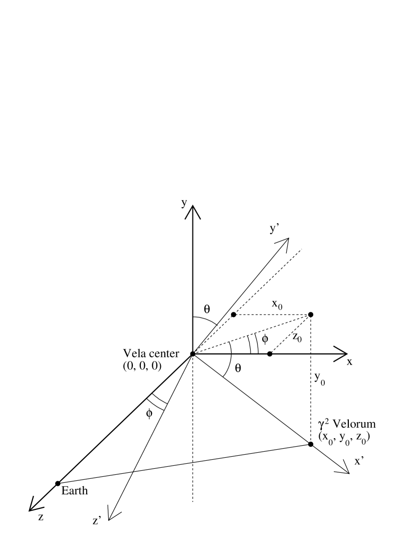
Figure 1: Definition of coordinate systems $\mathbf{K}$ and $\mathbf{K^{\prime}}$. See text for explanation.

For given coordinates $(x_{0},y_{0},z_{0})$ of $\gamma^{2}$Velorum in the $\mathbf{K}$-frame the rotation angles $\phi$ and $\theta$ can be estimated as

$$\tan\phi =\frac{\lvert z_{0}\rvert}{\lvert x_{0}\rvert},$$

$$\tan\theta =\frac{\lvert y_{0}\rvert}{\sqrt{x_{0}^{2}+z_{0}^{2}}}.$$ (3)

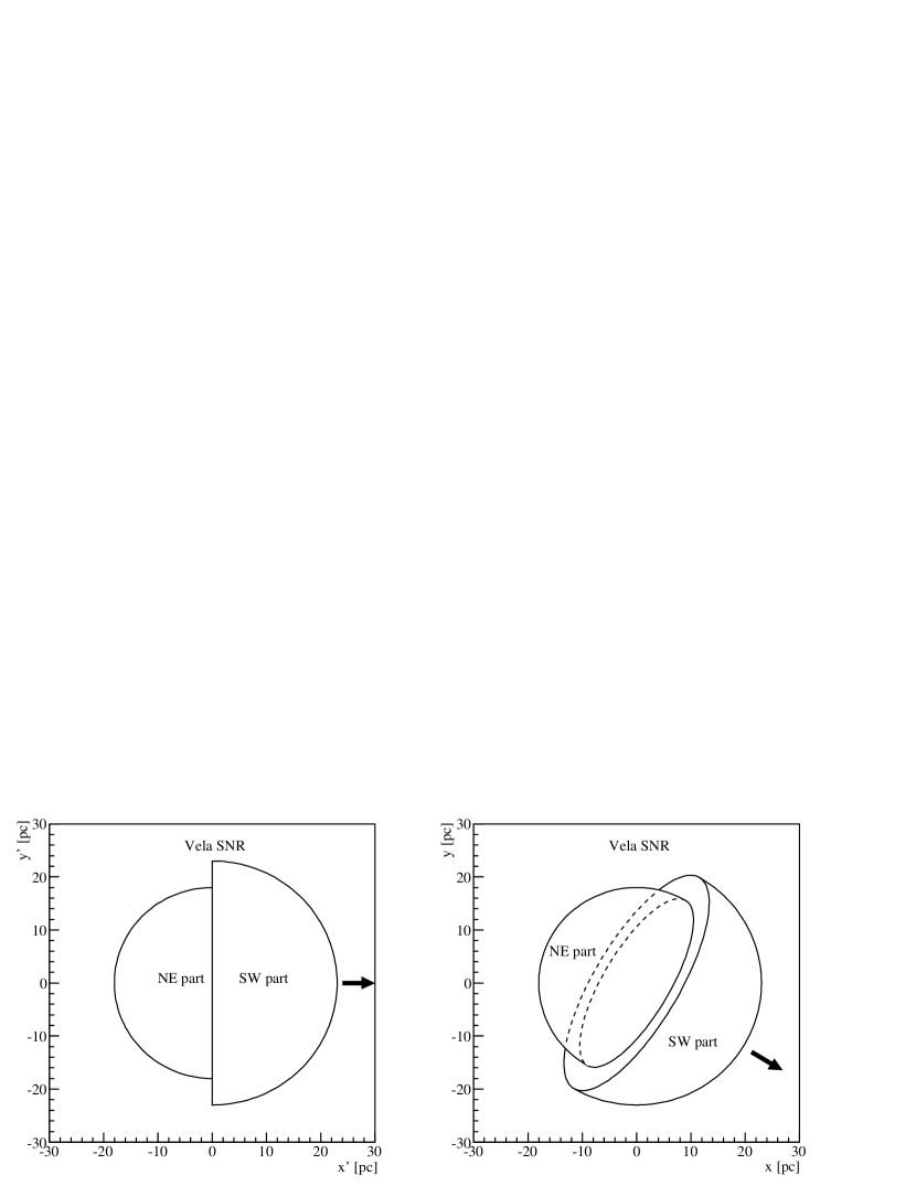
Figure 2: A schematic illustration of the $xy$-projection of the Vela SNR in $\mathbf{K^{\prime}}$ (left) and $\mathbf{K}$ (right) coordinate systems. The direction towards the position of $\gamma^{2}$Velorum is shown with an arrow.

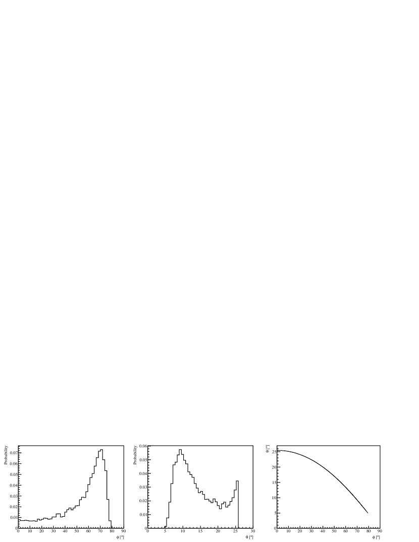
Figure 3: Distributions of rotation angles $\phi$ (left panel) and $\theta$ (central panel) obtained for the known estimates of distances to the Vela SNR and $\gamma^{2}$Velorum (see text for explanation). On the right panel the mutual dependence of rotation angles is shown.

In turn, $x_{0}$, $y_{0}$ and $z_{0}$ can be calculated using known distances and equatorial coordinates of the sources by transformation equations:

$$x_{0} =D_{\gamma^{2}\mathrm{Vel}}\cos\delta_{\mathrm{Vela}}\sin(\alpha_{\mathrm{Vela}}-\alpha_{\gamma^{2}\mathrm{Vel}}),$$

$$y_{0} =D_{\gamma^{2}\mathrm{Vel}}\sin(\delta_{\gamma^{2}\mathrm{Vel}}-\delta_{\mathrm{Vela}}),$$ (4)

$$z_{0} =D_{\mathrm{Vela}}-D_{\gamma^{2}\mathrm{Vel}}\cos\Delta,$$

where $\Delta$ is the angular distance between Vela and $\gamma^{2}$Velorum which is given by

$$\cos\Delta=\sin\delta_{\mathrm{Vela}}\sin\delta_{\gamma^{2}\mathrm{Vel}}+\cos\delta_{\mathrm{Vela}}\cos\delta_{\gamma^{2}\mathrm{Vel}}\cos(\alpha_{\mathrm{Vela}}-\alpha_{\gamma^{2}\mathrm{Vel}}).$$ (5)

Assuming that estimates of distances to the Vela SNR ($D_{\mathrm{Vela}}=287^{+19}_{-17}$ pc) and $\gamma^{2}$Velorum ($D_{\gamma^{2}\mathrm{Vel}}=334^{+40}_{-32}$ pc) follow asymmetric Gaussian distributions and asymmetric errors correspond to standard deviations of the distribution, one can obtain distributions of the rotation angles $\phi$ and $\theta$ from Eqs. (2-2) by varying distance estimates. Angle distributions presented in Fig. 3 (left and middle panels) show the probability of the true angle $\phi_{\mathrm{true}}/\theta_{\mathrm{true}}$ being in the range of angles $(\phi+\delta\phi)/(\theta+\delta\theta)$. Each histogram contains $50$ bins, i.e. $\delta\phi=1.8^{\circ}$ and $\delta\theta=0.6^{\circ}$. By calculating the mode for each distribution the most probable values of rotation angles $\phi$ and $\theta$ can be estimated

$$\phi_{0} =71.1\mbox{${}^{\circ}$}\pm 0.9\mbox{${}^{\circ}$}, \theta_{0} =9.3\mbox{${}^{\circ}$}\pm 0.3\mbox{${}^{\circ}$}.$$ (6)

The angles $\phi$ and $\theta$ are correlated and their mutual dependence is shown in the right panel of Fig. 3.

3 Radio emission from the spherical SNR with the uniform electron distribution

The radio emission from the Vela SNR shows an indication of the brightening towards the center which is not usually expected in the shell-like SNRs, where electrons emitting synchrotron radiation are accelerated at the main shock and are concentrated close to the edge of the remnant. In the case of the Vela SNR, the radio luminosity grows towards the center of the remnant featuring several localized maxima within the SNR. Such morphology suggests a close to uniform distribution of relativistic electrons inside the remnant. Possible reasons for such a distribution of electrons are discussed in the Section 5. In this section and the following one we investigate the radio emission from the SNR with a uniform distribution of relativistic electrons and apply this model to the case of the Vela SNR, considering it as a composition of two hemispheres with uniform distribution of relativistic electrons and magnetic field in each of them.

We assume that the distribution of the relativistic electron density $N_{\mathrm{e}}(\gamma)$ with energies follows a power law

$$\frac{dN_{\mathrm{e}}}{d\gamma}=K_{\mathrm{e}}\gamma^{-p},\gamma\geq\gamma_{\mathrm{min}},$$ (7)

where $\gamma$ is the electron Lorentz factor, $\gamma_{\mathrm{min}}$ is the minimal electron Lorentz factor, $K_{\mathrm{e}}$ is the normalization constant and $p$ is the electron spectral index. Then the overall synchrotron flux density at frequency $\nu$ from the spherical SNR located at distance $D$ can be calculated as (Rybicki & Lightman 1985)

$$S_{\nu}=$$

$$\frac{R^{3}}{3D^{2}}K_{\mathrm{e}}\frac{\sqrt{3}q^{3}B\sin{\theta}}{mc^{2}(p+1)}\Gamma\left(\frac{p}{4}+\frac{19}{12}\right)\Gamma\left(\frac{p}{4}-\frac{1}{12}\right)\left(\frac{2\pi mc}{qB\sin{\alpha}}\nu\right)^{-\frac{(p-1)}{2}},$$ (8)

where $B$ is the magnetic field, $R$ is the radius of the SNR, $q$ is the electron charge, $m$ is the electron mass, $c$ is the speed of light and $\alpha$ is the angle between the magnetic field and electron velocity. It is assumed that electron velocities are isotropically distributed and a root mean square value $\sin{\alpha}=\sqrt{2/3}$ can be used.

The flux density depends on three parameters, namely radius of the SNR $R$, magnetic field inside the SNR $B$ and constant $K_{\mathrm{e}}$. If the distance to the remnant is known the radius can be calculated directly from the angular size of the SNR.

The interior magnetic field is assumed to be determined mainly by shock-cloud interactions which result in vorticity and turbulence generation (see numerical calculations of shock-cloud interactions in Inoue et al. (2012) and references therein). It was shown in Inoue et al. (2012) that magnetic field amplification is determined by saturation at $\beta=8\pi P_{\mathrm{gas}}/B^{2}\sim 1$ (the equilibrium condition of the magnetic pressure and the thermal pressure of particles $P_{\mathrm{gas}}$). In the case of the Vela SNR the evaporated cloud material with spatially nearly uniform thermal pressure fills up practically all the volume of the remnant, therefore the magnetic field will be uniform within the remnant and can be estimated as

$$B=\sqrt{8\pi n_{\mathrm{tot}}k_{\mathrm{B}}T},$$ (9)

where $n_{\mathrm{tot}}=n/\mu$ is the total number density of electrons and nuclei, $n$ is the nucleon number density, $\mu=16/27$ is the molar mass, and $T$ is the kinetic gas temperature inside the remnant.

Finally, to calculate $K_{\mathrm{e}}$ one should know the total energy in relativistic electrons $E_{\mathrm{e}}$ and the size of the remnant. The total energy in electrons is given by the integration of the electron energy spectrum over all electron energies and over the volume of the remnant

$$E_{\mathrm{e}}=\iint mc^{2}\gamma\frac{dN_{\mathrm{e}}}{d\gamma}d\gamma dV=\frac{4}{3}\pi R^{3}mc^{2}K_{\mathrm{e}}\int_{\gamma_{\mathrm{min}}}^{\infty}\gamma^{-p+1}d\gamma.$$ (10)

Then parameter $K_{\mathrm{e}}$ can be expressed as

$$K_{\mathrm{e}}=\frac{E_{\mathrm{e}}}{\frac{4}{3}\pi R^{3}mc^{2}\int_{\gamma_{\mathrm{min}}}^{\infty}\gamma^{-p+1}d\gamma},\,(p>2).$$ (11)

4 Radio emission from the Vela SNR

We assume that the explosion of the supernova was spherically symmetrical. In this scenario the energy transferred to relativistic electrons in the SW and NE parts of the remnant would be the same and equal to a half of the total energy in electrons $E_{\mathrm{e}}$. Since the SW and NE parts of the remnant have different size, relativistic electron densities in these parts would be also different

$$N_{\mathrm{e,\,SW}}(\gamma\geq\gamma_{\mathrm{min}}) =K_{\mathrm{e,\,SW}}\int_{\gamma_{\mathrm{min}}}^{\infty}\gamma^{-p}d\gamma,$$

$$N_{\mathrm{e,\,NE}}(\gamma\geq\gamma_{\mathrm{min}}) =K_{\mathrm{e,\,NE}}\int_{\gamma_{\mathrm{min}}}^{\infty}\gamma^{-p}d\gamma,$$ (12)

where parameter $K_{\mathrm{e,\,SW/NE}}$ is dependent on the size of the hemisphere and can be estimated from Eq. 11 for $R_{\mathrm{SW/NE}}$. We assume that the minimal energy of electrons is $\gamma_{\mathrm{min}}mc^{2}=100$ MeV. The total energy in electrons $E_{\mathrm{e}}$ and the electron spectral index can be derived from the observational data as discussed below. Magnetic fields inside the remnant $B_{\mathrm{NE/SW}}$ can be calculated using Eq. (9) and estimates of nucleon number density $n_{\mathrm{hot}}^{\mathrm{NE/SW}}$ and kinetic temperature $T_{\mathrm{hot}}^{\mathrm{NE/SW}}$ of the hot component (dominant across the remnant) listed in the Table 1. In the NE part of the remnant the magnetic field is $B_{\mathrm{NE}}=46\,\mu$G, while in the SW part it is $B_{\mathrm{SW}}=30\,\mu$G.

4.1 Integrated flux density

By fitting the model flux density (Eq. (3)) to the observational data one can calculate the total energy in electrons $E_{\mathrm{e}}$ and the electron spectral index $p$ for the assumed minimal electron Lorentz factor $\gamma_{\mathrm{min}}$. Alvarez et al. (2001) provide the flux density from the whole remnant $S_{XYZ}$ and flux densities from localized emission regions $S_{X}$, $S_{Y}$ and $S_{Z}$ from Vela X, Vela Y and Vela Z, respectively (see Tab. 2 therein). The ratio of the integrated flux density $S_{XYZ}$ to the sum of components $S_{X}+S_{Y}+S_{Z}$ shows appropriate self-consistency. Vela X is the PWN associated with the Vela pulsar and should not be taken into account for the study of the emission from the Vela SNR itself. Therefore, the flux density from the whole remnant $S_{XYZ}$ which includes the emission from the PWN Vela X cannot be used here. The emission from Vela Y and Vela Z comes mainly from the NE part of the remnant. Flux densities of Vela Y and Vela Z were summed up and the resulting cumulative flux density (Fig. 4) is assumed to be the flux density of the NE part of the Vela SNR. The model fit of the data (solid line in Fig. 4) results in the following values for the fitting parameters

$$p =2.47\pm 0.09,$$ (13)

$$E_{\mathrm{e}} =(2.4\pm 0.2)\times 10^{47}\,\mathrm{erg},$$ (14)

which corresponds to a fraction of the total explosion energy transferred to electrons of

$$\epsilon_{\mathrm{e}}=E_{\mathrm{e}}/E_{\mathrm{SN}}=(1.7\pm 0.1)\times 10^{-3}$$ (15)

which is close to a typical value, expected for SNRs (see e.g. Katz & Waxman (2008); Gabici (2008)). Flux densities at 29.9 MHz and 34.5 MHz were not fit since they show some indication of absorption (Alvarez et al. 2001). For the known $p$ and $E_{\mathrm{e}}$, the relativistic electron densities and parameters $K_{\mathrm{e}}$ for both, NE and SW, parts of the remnant can be calculated. They are presented in Table 2.

Figure 4: Sum of the integrated flux density spectra from Vela Y and Vela Z, presented in Alvarez et al. (2001). The straight line represents a model fit to the data.

Table 2: Physical parameters of the relativistic electron population inside the Vela SNR.

Obtained from	Parameter	NE	SW
a fit of the radio spectrum	$p$	$2.47\pm 0.09$
	$E_{\mathrm{e}}$ [erg]	$(2.4\pm 0.2)\times 10^{47}$
	$\epsilon_{\mathrm{e}}$	$(1.7\pm 0.1)\times 10^{-3}$
	$K_{\mathrm{e}}$ [cm-3]	$2.4\times 10^{-6}$	$1.2\times 10^{-6}$
	$N_{\mathrm{e}}$ [cm-3]	$0.7\times 10^{-9}$	$0.3\times 10^{-9}$
a flux density at 408 MHz	$E_{\mathrm{e}}$ [erg]	$(3.6\pm 0.5)\times 10^{47}$
	$\epsilon_{\mathrm{e}}$	$(2.6\pm 0.3)\times 10^{-3}$
	$K_{\mathrm{e}}$ [cm-3]	$3.6\times 10^{-6}$	$1.7\times 10^{-6}$
	$N_{\mathrm{e}}$ [cm-3]	$1.1\times 10^{-9}$	$0.5\times 10^{-9}$

4.2 Morphology

The brightness temperature map of the Vela SNR at 408 MHz in equatorial coordinates was simulated using the geometrical model presented in Section 2. The emission was modelled in 3D in the $\mathbf{K^{\prime}}$ coordinate system, treating every unit volume as a separate emitter. Then the 3D-model of the remnant was converted to the $\mathbf{K}$ coordinate system and projected onto the $xy$-plane. Finally, the $xy$-plane was converted to the equatorial coordinates as described in the Section 2.

Primarily, the simulation was performed using estimates of the physical parameters of the electron population obtained from the fit of the observed radio spectrum (see the subsection above) and the mode values $\phi_{0}$ and $\theta_{0}$ of rotation angles $\phi$ and $\theta$. In the top left panel of Fig. 5 the simulated temperature brightness map for these values is shown. The color corresponds to the brightness temperature in K. The brightness temperature distribution is determined by the integration of the radio emission along the line of sight. The radio emission is stronger in the NE hemisphere of the remnant due to the higher density of relativistic electrons and stronger magnetic field. The emission would peak in the center of the remnant in the two limiting cases, namely, when the center of the Vela SNR and $\gamma^{2}$Velorum are located on the same line of sight, i.e. $\phi=90\mbox{${}^{\circ}$}$ and $\theta=0\mbox{${}^{\circ}$}$ and in the case when the Vela SNR center$-$$\gamma^{2}$Velorum symmetry axis is perpendicular to the line of sight, i.e. the Vela SNR and $\gamma^{2}$Velorum are located at the same distance and $\phi=0\mbox{${}^{\circ}$}$. In the intermediate case $0<\phi<90\mbox{${}^{\circ}$}$ the peak of the brightness temperature is shifted to the NE part of the remnant, as shown in Fig. 5 (top left panel) for the case of the most probable values of $\phi=71.1\mbox{${}^{\circ}$}$ and $\theta=9.3\mbox{${}^{\circ}$}$.

For $\phi\leq 40\mbox{${}^{\circ}$}$, a second, considerably fainter, peak appears in the SW part of the remnant. It is not seen for $\phi>40\mbox{${}^{\circ}$}$ due to the overlapping effect, which causes the contamination of the SW part of the remnant by the radio emission from the NE hemisphere. Remarkably, these two theoretically predicted peaks correspond to the observed morphology of the brightness temperature distribution in the Vela SNR - the existence of ”hot spots” in both, the NE (two close localized regions of Vela Y and Vela Z) and SW (two peaks of Vela W) parts of the remnant. The peaks of the emission regions Vela Y and Vela Z are shown as down- and up-pointing triangles, respectively, and the peaks of the Vela W region are shown as filled circles in each map in Fig. 5. For another combination of angles $\phi=35\mbox{${}^{\circ}$}$ and $\theta=21\mbox{${}^{\circ}$}$, which is also compatible with estimates for the distances to the Vela SNR and $\gamma^{2}$Velorum, the positions of the simulated brightness temperature peaks coincide with the observed localized regions (Fig 5 top right), suggesting that the complicated morphology of the Vela SNR might be a result of superimposed emission in the system with a specific spatial orientation.

Modeled peak brightness temperatures on the top right panel of Fig. 5 are slightly lower than the observed brightness temperatures of the Vela Y, Vela Z, and Vela W peaks. As reported by Alvarez et al. (2001) the brightness temperature of the Vela Y and Vela Z peaks is about 90 K and the brightness temperature of Vela W peaks is 35$-$40 K,while on the simulated map peak temperatures are $\sim 50$ K and $\sim 15$ K, respectively. This difference is expected given that the observed cumulative Vela Y and Vela Z flux density at 408 MHz is $1.5$ times higer than the model fit to the data at this frequency (Fig. 4). Therefore, in order to be able to accurately compare the simulated and observed brightness temperature distributions one has to derive the total energy in electrons directly from the observed flux density at 408 MHz. The spectral index is assumed to be $p=2.47$ as obtained in a fit. The derived physical parameters of the electron population are presented in Table 2. Using these new estimates we simulate the brightness temperature distribution for the two sets of $\phi$ and $\theta$ discussed above (Fig. 5 bottom left and bottom right panels). In this case, the simulated peak brightness temperatures for the combination of angles $\phi=35\mbox{${}^{\circ}$}$ and $\theta=21\mbox{${}^{\circ}$}$ (Fig. 5 bottom right) are in a good agreement with the observational results. The brightness temperature of the NE peak is about 80 K and the brightness temperature of the SW peak is about 25 K. This consistency with the observational data is another confirmation of the validity of our model.

Figure 5: Simulated brightness temperature maps at 408 MHz in equatorial coordinates overlaid by galactic coordinates. Maps are calculated for $\epsilon_{\mathrm{e}}=1.7\times 10^{-3}$ (two upper panels) and $\epsilon_{\mathrm{e}}=2.6\times 10^{-3}$ (two lower panels). Two sets of rotation angles are considered: most probable values $\phi=71.1\mbox{${}^{\circ}$}$, $\theta=9.3\mbox{${}^{\circ}$}$ (two left panels) and values which describe observational data the best $\phi=35\mbox{${}^{\circ}$}$, $\theta=21\mbox{${}^{\circ}$}$ (two right panels). The color reflects the brightness temperature in K. The angular resoulution of the modeled brightness temperature distributions is $4^{\prime}$. In each map white filled down- and up-pointing triangles denote peak locations of Vela Y an Vela Z correspondingly, two white filled circles show locations of two peaks of Vela W, a white filled square denotes the position of the Vela X peak (Alvarez et al. 2001), and a cross reflects the location of $\gamma^{2}$Velorum. The bottom right map which represents ”the best fit” scenario is overlaid with observed 408 MHz radio contours with $51^{\prime}$ angular resolution from Haslam et al. (1982). The contours represent the brightness temperature in K and the steps are 4 K from 40 K to 100 K, 10 K from 100 K to 150 K and 25 K further on, the contours of 60 and 100 K are shown with the bold lines. Contrary to the map presented in Alvarez et al. (2001), the galactic background is not removed, which explains the difference in values of the brightness temperature. Alvarez et al. (2001) adopted two background temperatures of 50 and 60 K at 408 MHz. Besides Vela X in the centre, additional prominent (RCW 38 ($\alpha=08^{h}59^{m},\delta=-47^{\circ}32^{\prime}$), Puppis A ($\alpha=08^{h}23^{m},\delta=-42^{\circ}42^{\prime}$)) and weaker compact sources (RCW 36, RCW 33 and RCW 27 clockwise along the NE-North surface) are visible.

5 Discussion

5.1 Uniform distribution of relativistic electrons

A typical middle-aged SNR in the adiabatic stage of evolution is a powerful source of both thermal X-ray and nonthermal synchrotron radio emission. A strong shock wave compresses and heats the interstellar gas up to keV temperatures creating a shell-like X-ray morphology due to the concentration of the shocked plasma downstream of the shock front. At the same time the shock wave accelerates charged particles, electrons, protons and nuclei, to ultrarelativistic energies via the diffusive shock acceleration mechanism. Since both the magnetic field and relativistic electrons are also concentrated downstream the shock front, the radio-brightness distribution of the SNR would also feature a shell-like morphology.

Although the Vela SNR is in the adiabatic stage of evolution it does not show the usual behavior of, so called, Sedov SNRs as described above. Its dynamics is mainly determined by the interaction of the SN ejecta with numerous clouds with a volume averaged density considerably higher than the density of the intercloud ISM (Sushch et al. (2011) and references therein). While in the adiabatic Sedov SNR the hot postshock plasma is a swept up and heated ISM gas, in the Vela SNR the hot postshock plasma is predominantly the heated and evaporated cloud gas. This difference has a prominent role in the postshock distribution of relativistic electrons. Due to the low ISM density the transfer of the SN explosion energy into the ISM (and, in turn, into the cosmic ray acceleration), is small while the main channel of the ejecta kinetic energy dissipation is the interaction with clouds through the heating and evaporating of the cloud gas.

Primarily, the dominant process which takes place in the Vela SNR is the interaction between the ejecta and clouds with generation of the transmitted shock in the cloud and the reflected shock in the ejecta. Due to the large cloud/intercloud ISM density contrast for the expected Vela SN ejecta mass of $M_{\mathrm{ej}}\sim 10\,M_{\odot}$ (Limongi & Chieffi 2006) and velocity of $V_{\mathrm{ej}}=\sqrt{2E_{SN}/M_{\mathrm{ej}}}\sim 1.5\times 10^{3}$ km/s the main dissipation of the kinetic energy of the ejecta takes place at reverse shocks generated in the ejecta-clouds interaction. Due to the low temperature of the ejecta plasma (zero pressure in the analytical treatment of Truelove & McKee (1999) and $T_{\mathrm{ej}}\sim 10^{4}$ K in numerical simulations of Moriya et al. (2013)), the sonic Mach number should be high (up to 100-150 for $T_{\mathrm{ej}}\sim 10^{4}$ K) and, thus, the reverse shock will be a region of effective CR (including relativistic electrons) acceleration. It is more complicated to estimate parameters of the transmitted shocks, where the transmitted shock velocity depends on the ejecta and cloud densities $V_{\mathrm{tr}}\sim V_{\mathrm{ej}}\sqrt{\rho_{\mathrm{ej}}/\rho_{\mathrm{cl}}}$. For the expected cloud radius $r_{\mathrm{cl}}\sim 0.05$ pc and the number densities $n_{\mathrm{cl}}^{\mathrm{core}}\sim 100\,\mathrm{cm}^{-3}$ and $n_{\mathrm{cl}}^{\mathrm{corona}}\sim 10\,\mathrm{cm}^{-3}$ in the two-component approximation in which the cloud consists of a dense core and a corona around the core (Miceli et al. 2006), at the initial phase of the ejecta-cloud interaction the velocity of the transmitted shock should be high enough for the effective particle acceleration, but it will decrease with the distance from the point of the SN explosion due to the decrease of the ejecta density.

With time, the main shock will form. The downstream gas will be dominated by the evaporated plasma with a contribution of the ejecta plasma reheated by the reverse shock. The contribution of the shocked intercloud plasma is negliglible. Hot postshock plasma will additionally heat and destroy clouds by thermal conductivity and generating transmitting shocks.

The total mass of the ejecta and evaporated clouds inside the Vela SNR is about $30\/M_{\odot}$ (see Table 1), i.e. the mass of evaporated clouds is only about twice the ejecta mass $M_{\mathrm{ej}}\sim 10\,M_{\odot}$, suggesting that the direct ejecta-cloud interaction was effective and, in turn, that effective acceleration of relativistic electrons at strong reverse shocks took place. The close to uniform distribution of clouds in the ISM leads to a uniform system of strong reverse shocks and, thus, to a nearly uniform distribution of relativistic electrons inside the Vela SNR. The close to uniform distribution of the relativistic electrons inside the Vela SNR remains with time due to the strong turbulent magnetic field (see Section 3), which restrains the diffusion from the acceleration region. At the same time, the large magnetic field of the Vela SNR (about $50\mu$G) does not modify the energy spectrum of relativistic electrons radiated in the range of 30-2700 MHz. The characteristic frequency of a photon emitted by an electron with energy $\epsilon_{\mathrm{e}}$ is given by (Rybicki & Lightman 1985)

$$\nu_{\mathrm{ch}}=0.29\frac{3q\sin{\alpha}}{4\pi m^{3}c^{5}}\epsilon_{\mathrm{e}}^{2}B\simeq 190\left[\frac{\epsilon_{\mathrm{e}}}{1\,\mathrm{GeV}}\right]^{2}\left[\frac{B}{50\,\mu\mathrm{G}}\right]\mathrm{[MHz]},$$ (16)

i.e. to emit a 2700 MHz photon an electron with energy $\epsilon_{\mathrm{e},2700}\sim 3.8$ GeV is needed. The cooling time for synchrotron radiation of such electron is (Blumenthal & Gould 1970)

$$t_{\mathrm{syn}}=1.3\times 10^{6}\left[\frac{\epsilon_{\mathrm{e}}}{4\,\mathrm{GeV}}\right]^{-1}\left[\frac{B}{50\,\mu\mathrm{G}}\right]^{-2}\mathrm{[y]}.$$ (17)

This time is much longer than the estimate of the age of the Vela SNR (regardless the uncertainty which occurs due to the low braking index of the pulsar), suggesting that electrons can indeed survive over the time inside the remnant emitting synchrotron radiation.

5.2 Local discrepancies of the modelled and observed morphology

The modelled brightness temperature map of the Vela SNR predicts two local elongated peaks, one in the NE part of the remnant and one in the SW part of the remnant. Observations show that there are two localized peaks in each part of the remnant. But the identical brightness temperatures of the two NE peaks, Vela Y and Vela Z, and the two SW peaks, Vela W, suggest that physically the two observed peaks in each part of the remnant have the same nature and are two parts of the same peak which could be splitted due to some deviations from our idealised symmetric model. Another small discrepancy between the modelled and observed morphologies is that the peaks of Vela W are slightly offset from the modelled peak in the SW part of the remnant. One of the most natural reasons of these discrepancies is that the initial distribution of clouds and, thus, relativistic electrons does not necessarily have to be uniform.

Both discrepancies can be naturally explained also by the existence of the PWN Vela X inside the remnant. The peak of the radio emission from Vela X, as reported by Alvarez et al. (2001), is indicated with a filled square in all maps in Fig. 5. Indeed, the expansion of the PWN can change the distribution of the internal gas and the cloud matter inside the Vela SNR ”pushing” them to the outer regions of the remnant. This, in turn, would change the distribution of relativistic electrons responsible for the synchrotron radiation, if they are accelerated at local shocks generated in clouds. However, the evolution and expansion of Vela X is not yet well understood. The PWN features different morphologies at different wavebands. At radio and GeV energies an extended ($2\mbox{${}^{\circ}$}\times 3\mbox{${}^{\circ}$}$) ”halo” emission is observed featuring a ”two-wing” structure (Grondin et al. 2013), which is located mostly to the south of the Vela pulsar (as seen in the equatorial coordinates). While the X-ray observations by ROSAT revealed a much smaller ($45^{\prime}\times 12^{\prime}$) emission region (”cocoon”) (Markwardt & Ögelman 1995). Subsequent high resolution X-ray observations with Chandra revealed a structure of the X-ray emission as a composition of two toroidal arcs ($17^{\prime\prime}$ and $30^{\prime\prime}$ away from the pulsar) and a $4^{\prime}$-long collimated jet (Helfand et al. 2001). Finally, in the TeV range, emission spatially coincident with both, halo and cocoon, is detected (Aharonian et al. 2006; Abramowski et al. 2012). According to the morphology of the halo emission from Vela X, the interaction of the PWN with the internal medium of the remnant is expected to provide a more important effect on the SW hemisphere of the remnant, since the main part of the PWN is located there. Expanding towards the position of Vela W peaks, the PWN may cause an increase of the electron density and, thus, the enhancement of the synchrotron emission in that region.

Another effect, which may be responsible for the distribution of electrons inside the remnant is the propagation of the reverse shock inside the remnant. It is argued in the literature that the reverse shock of the SNR may be the reason of the asymmetrical structure of Vela X with respect to the pulsar position (Blondin et al. 2001). Due to the difference of the properties of the ambient medium on the NE and SW sides of the remnant it is possible that the reversed shock was formed earlier in the NE part of the SNR and reached the PWN Vela X suppressing it, while in the SW part of the remnant still no interaction of the PWN with the reverse shock is established (Blondin et al. 2001). If this is the case, then the reverse shock should also influence the distribution of electrons and the intensity of the emission.

6 Summary

The radio emission from the Vela SNR was simulated in the framework of the hydrodynamical model presented in Sushch et al. (2011). This model is based on two hypotheses:

• the progenitor of the Vela SNR exploded at the border of the stellar wind bubble of the nearby binary system $\gamma^{2}$Velorum which causes the remnant to expand into two media with different densities,

• the remnant expands into the inhomogeneous medium in which the main bulk of mass is concentrated in small clouds.

Originally the model was elaborated to explain a peculiar X-ray emission from the source. In this paper, we showed that the observed radio flux from the remnant can also be well explained within this model giving it a further observational support.

It was shown that the complicated radio morphology which features several localized emission regions can be explained by the relative positioning of the Vela SNR and $\gamma^{2}$Velorum, assuming that relativistic electrons responsible for the synchrotron radio emission are distributed uniformly inside the remnant. The expected observed image of the Vela SNR depends on how these two objects are positioned relative to each other. We show that for rotation angles $\phi=35\mbox{${}^{\circ}$}$ and $\theta=21\mbox{${}^{\circ}$}$ the expected brightness temperature map of the remnant would feature two peaks in the NE and SW parts of the remnant, which are coincident with the observed localised emission regions Vela Y, Vela Z and Vela W. The simulated brightness temperatures of the peaks are in good agreement with the observed brightness temperatures in local emission regions.

We also argue that the PWN Vela X located inside the remnant, which was not taken into account in this study, may play a notable role in the distribution of relativistic electrons within the remnant and, thus, in the morphology of the radio emission of the Vela Y, Vela Z and Vela W regions. The detailed model of the Vela X contribution to the radio emission of Vela SNR will be considered elsewhere.