Investigating amorphous order in stable glasses by random pinning

Abstract

We use a random pinning procedure to investigate stable glassy states associated with large deviations of the activity in a model glass-former. We pin particles both from active (equilibrium) configurations and from stable (inactive) glassy states. By comparing the distribution of the overlap between states that share pinned particles, we infer that the inactive states are characterised by a structural length scale that is comparable with the system size. This is a manifestation of amorphous order in these glassy states, which helps to explain their stability.

Glassy materials are stable and appear to be solid, but their molecular structures closely resemble those of liquids nagel-review ; deb-review . Reconciling these two observations is a central challenge if the properties of these important materials are to be understood. To this end, a useful concept is amorphous order, which means that while the structure of a glass appears highly disordered, there may nevertheless be strong correlations between particles, extending over significant length scales KL ; BB-ktw-2004 ; montanari06 , and leading to glassy behavior adam-gibbs ; ktw ; BB-ktw-2004 . These correlations can be revealed (for example) by point-to-set correlation functions berthier-pin2012 ; biroli-pin ; berthier-kob-pin2013 ; cavagna08 ; berthier-silvio . Alternatively, given that the most significant differences between liquid and glass states appear in dynamical measurements, one may argue that a useful description of the glass transition should focus on particle dynamics GC-2003 ; GC-annrev-2010 . Recent studies based on this hypothesis have revealed non-equilibrium phase transitions kcm-transition ; hedges09 that occur when systems are biased to suppress particle motion, in “$s$-ensembles”. Here, we use random pinning (point-to-set) measurements berthier-pin2012 ; biroli-pin ; berthier-kob-pin2013 to show that while these stable glasses were found by analysing their dynamical properties, they also exhibit strong amorphous order. Hence, we argue that the dynamical approach of the $s$-ensemble and the structural idea of growing amorphous order are not contradictory jack10-rom : rather, they offer complementary routes biroli-garrahan by which theories of the glass transition may be developed and refined.

We consider the well-studied glass-forming liquid of Kob and Andersen ka95 . As well as its equilibrium state, this system exhibits a non-equilibrium ‘inactive phase’ hedges09 , which is extremely stable jack11-stable , and is found by biasing dynamical trajectories to lower than average activity. The stable glassy states that we consider were taken from this inactive phase, for a system of $N=150$ particles. Full details are given in Supplementary Information (SI). The natural unit of length in the system is the diameter $\sigma$ of the larger particles (species A), the system size is $L=5\sigma$, and all results shown are for temperature $T=0.6$ (in units of the AA-interaction energy), for which the equilibrium state is a weakly supercooled fluid. The system evolves by overdamped (Monte Carlo) dynamics berthier-mc2007 , which gives results for structural relaxation in quantitative agreement with molecular dynamics berthier-mc2007 ; hedges09 . Time is measured in units of $\Delta t=\sigma^{2}/D_{0}$, where $D_{0}$ is the diffusion constant of a free particle.

To analyse the connection between amorphous order and the stability of inactive states, we use a random pinning procedure berthier-pin2012 ; biroli-pin . For a given reference configuration, we fix the position of each particle with probability $c$, arriving at a template: a set of approximately $cN$ pinned particles. The remaining (unpinned) particles then move as normal in the presence of the frozen template. If the reference configuration comes from a highly-ordered state, one expects a strong influence of the template on the dynamic and thermodynamic properties of the system. For example, in a perfectly crystalline sample, a template containing just three particles is sufficient to determine the lattice orientation and hence the positions of all other particles. More generally, if a template containing a small fraction of particles has a strong influence on the liquid structure, this indicates that the correlations among particle positions are strong, and hence that the system is ordered, even if this order is not apparent from (for example) two-point density correlations.

To analyse the influence of the template, we require a measure of similarity between configurations. To obtain useful measurements for configurations where particle indices are permuted but the structure remains similar, we divide the system into a cubic grid of cells of linear size $\ell=(L/10)=0.5\sigma$ berthier-pin2012 . Let $n_{i}$ be the number of mobile (unpinned) particles of type A in cell $i$. Then, if configurations $\mathcal{C}$ and $\mathcal{C}^{\prime}$ have cell occupancies $\{n_{i}\}$ and $\{n_{i}^{\prime}\}$, their (normalised) overlap is

$$Q(\mathcal{C},\mathcal{C}^{\prime})=\frac{1}{M}\sum_{i}\frac{n_{i}n_{i}^{\prime}-\langle n_{i}\rangle^{2}}{\langle n_{i}^{2}\rangle-\langle n_{i}\rangle^{2}}.$$ (1)

If $\mathcal{C}$ and $\mathcal{C}^{\prime}$ are identical then $\langle Q\rangle=1$ while for independent random configurations $\langle Q\rangle=0$.

In equilibrium studies of pinning berthier-pin2012 ; biroli-pin ; berthier-kob-pin2013 ; charb-prl2012 ; krakoviack2010 ; kurzidim2011 ; kim-pin2011 ; karmarkar2012 ; jack-plaq-pin ; jack-pin-chi4 one begins by drawing an equilibrium reference configuration $\mathcal{C}_{0}$, from which each particle is pinned with probability $c$. Then, a second configuration $\mathcal{C}$ is generated, which includes the pinned particles from $\mathcal{C}_{0}$, while the remaining particles are equilibrated in the presence of this template. On repeating this procedure many times, one may build up a distribution $p_{\rm eq}(Q|c)$ for the overlap $Q=Q(\mathcal{C}_{0},\mathcal{C})$. The associated ensemble is discussed in SI. We emphasise that this is a static (thermodynamic) procedure, in that $p_{\rm eq}(Q|c)$ depends only on the Boltzmann distribution (or potential energy surface) of the system.

To measure amorphous order for inactive states, we draw reference configurations $\mathcal{C}_{0}$ from trajectories of the model that are biased to lower than average dynamical activity – full details are given in SI. The inactive state is in contact with a thermostat at $T=0.6$ at all times, so the natural comparison is between the inactive state and an equilibrium state at that temperature. Starting from the inactive reference configurations, we use the same pinning procedure as described above, which results in a different distribution of the overlap, denoted by $p_{\rm in}(Q|c)$. If the inactive states have increased amorphous order as compared to equilibrium, one expects significant differences between $p_{\rm eq}(Q|c)$ and $p_{\rm in}(Q|c)$.

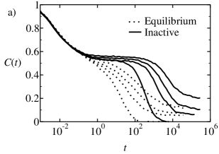
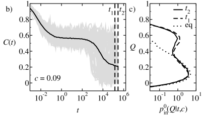
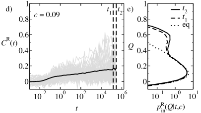
Figure 1: (a) $C(t)$, calculated from equilibrium and inactive reference configurations. From left to right $c=0.00,0.05,0.07,0.09$. (b) For an inactive reference state and $c=0.09$, the average overlap $C(t)$ (black) and plots of $Q(\mathcal{C}_{0},\mathcal{C}_{t})$ for representative trajectories (gray). (c) Distributions of $Q(\mathcal{C}_{0},\mathcal{C}_{t})$ (gray data from (b)) at the times indicated, compared with $p^{0}_{\rm{eq}}(Q|t,c)$ for an equilibrium reference state, at $c=0.09$ and $t=t_{2}/4$, representative of the long-time limit. (d,e) Data analogous to (c,d), except that dynamical trajectories were started from configurations in which the positions of unpinned particles were ‘randomised’ at $t=0$ (see text). For all histograms, results are accumulated over time windows ending at the indicated times: the windows are long enough to enable precise measurements but short enough that they do not significantly affect the shapes of the distributions.

To infer the form of $p_{\rm in}(Q|c)$ and $p_{\rm eq}(Q|c)$, we conducted dynamical simulations. For a given reference configuration $\mathcal{C}_{0}$ and a given template, we simulated dynamical trajectories starting from $\mathcal{C}_{0}$. This leads to a time-dependent overlap $Q(\mathcal{C}_{0},\mathcal{C}_{t})$, where $\mathcal{C}_{t}$ is the configuration of the system at time $t$. We then repeat the procedure for many different templates and different reference configurations. Fig. 1(a) shows the time-dependent average overlap $C(t)=\langle Q(\mathcal{C}_{0},\mathcal{C}_{t})\rangle$, comparing the behavior for equilibrium and inactive reference configurations. As in jack11-stable , the dynamical relaxation from inactive states is much slower than equilibrium relaxation, even in the absence of pinning. Also, as $c$ is increased, the dynamical relaxation slows down, for both equilibrium and inactive reference states jack-pin-chi4 .

Fig. 1(b,c) indicates that the slow decay of $C(t)$ is associated with large fluctuations of $Q(\mathcal{C}_{0},\mathcal{C}_{t})$. For long times, the time-dependent distribution $p_{\rm in}^{0}(Q|t,c)$ of this overlap has a characteristic bimodal shape. In contrast, the distribution $p_{\rm eq}^{0}(Q|t,c)$, obtained under the same conditions, lacks the second peak at high-$Q$. The differences between these distributions are entirely due to the to the structural differences between the reference states (inactive or equilibrium) from which the pinned particles were selected. Further, the dynamics used here ensure (see SI) that $\lim_{t\to\infty}p_{\rm in}^{0}(Q|t,c)=p_{\rm in}(Q|c)$, which indicates that differences between the long-time limits of $p_{\rm in}^{0}(Q|t,c)$ and $p_{\rm eq}^{0}(Q|t,c)$ can be attributed to amorphous order, as measured by $p_{\rm eq}(Q|c)$ and $p_{\rm in}(Q|c)$. However, it is clear from Fig. 1 that $p_{\rm in}^{0}(Q|t,c)$ has not reached its large-$t$ limit, so we may not assume that the ‘dynamical’ distribution $p_{\rm in}^{0}(Q|t,c)$ reflects the form of the ‘static’ distribution of interest, $p_{\rm in}(Q|c)$. In particular, the secondary maximum at large-$Q$ in $p_{\rm in}^{0}(Q|t,c)$ might disappear on increasing $t$, as systems finally relax away from the reference configuration into other available states.

To address this point, we conducted simulations in which a template was fixed as before, after which the temperature was increased to $T=5.0$ and dynamics run for $t\approx 1000\Delta t$. This temperature is high enough that the mobile particles quickly decorrelate from their initial configuration. These ‘randomised’ states were then used as initial conditions for dynamical simulations (see hocky2012 for a similar idea). As before, we measure the distribution of the overlap between the reference $\mathcal{C}_{0}$ and the resulting time-dependent configurations $\mathcal{C}_{t}$. Let the distribution of this overlap be $p_{\rm in}^{\rm R}(Q|t,c)$ and let $C^{\rm R}(t)=\langle Q(\mathcal{C}_{0},\mathcal{C}_{t})\rangle$ be the average overlap for this distribution.

Results are shown in Fig. 1(d,e): the average overlap $C^{\rm R}(t)$ starts near zero (as expected for a randomised initial condition) and slowly increases, due to the influence of the template. Further, for large times, there are a substantial number of trajectories where the system spontaneously evolves into a state with large $Q$. This means that the frozen template (containing just $9\%$ of the particles) influences the system strongly enough that it has a significant probability of returning to the metastable state associated with the original reference configuration. As before, $p_{\rm in}^{\rm R}(Q|t,c)\to p_{\rm in}(Q|c)$ as $t\to\infty$ but this limit is not saturated. However, we see that while $p_{\rm in}^{\rm R}(Q|t,c)$ and $p_{\rm inac}^{0}(Q|t,c)$ are converging to the same limit, they do so from opposite directions, in that the original simulations start in the reference state $\mathcal{C}_{0}$ and evolve away from it, while the ‘randomised’ simulations start far from $\mathcal{C}_{0}$ and evolve back towards this reference state. Thus, a natural conjecture is that these two distributions give (approximate) upper and lower bounds on the limit distribution $p_{\rm in}(Q|c)$.

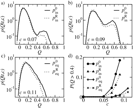
Figure 2: (a-c) Distributions of $Q(\mathcal{C}_{0},\mathcal{C}_{t})$. (a) $c=0.07$ for an inactive reference; (b) $c=0.09$, inactive reference; (c) equilibrium reference, for the relatively high pinning probability $c=0.11$ (results for lower $c$ are similarly unimodal). In (b), $t=t_{2}$ as indicated in Fig. 1b; for (a,c) the times are $3t_{2}/4$ and $t_{2}/4$ respectively. (d) Probability that the overlap $Q>0.4$, corresponding to the high-$Q$ peak in the distributions $p(Q|t,c)$, for equilibrium and inactive references.

Fig. 2 collates the relevant distributions. The key observation is that the inactive reference configurations lead to bimodal distributions of the overlap, while equilibrium reference configurations result in unimodal distributions, even for pinning fractions as high as $c=0.11$. We note also that the probability associated with the large-$Q$ peak in $p_{\rm in}(Q|t,c)$ rises in a strongly non-linear fashion, indicating the central role of many-body correlations szamel-pin2013 .

We now discuss how these numerical results shed light on the nature of amorphous order in these systems. It is natural to write

$$p(Q|c)=\mathrm{e}^{-N\beta V(Q,c)}$$ (2)

where $V(Q,c)$ is an effective potential, as used in mean-field theories of the glass transition franz-parisi-1997 , generalised to include the effect of the frozen templates. Within mean-field theories and below the onset temperature ($T_{\rm o}\approx 1$ for this model) one expects two peaks in $p(Q|c)$, as $Q$ is varied, and hence two minima in $V(Q,c)$. These correspond to the cases where $\mathcal{C}$ and $\mathcal{C}_{0}$ are in the same metastable state (high-$Q$) or in different states (low-$Q$). As $c$ is increased, one expects the low-$Q$ peak to be reduced, because cases where $\mathcal{C}$ is in a different state from $\mathcal{C}_{0}$ are not typically consistent with the frozen template. Within random first-order transition theory ktw , one additionally expects a phase transition at some critical concentration $c$ biroli-pin ; camma-pin-alpha , so that the high-$Q$ peak of $p(Q|c)$ dominates the distribution for $c>c^{*}$, while the low-$Q$ peak dominates for $c<c^{*}$.

If such phase transitions occur in randomly pinned systems, the distribution $P(Q|c)$ remains bimodal as the system size $N\to\infty$. Numerically, this can be inferred by a finite-size scaling analysis berthier-kob-pin2013 . However, the long time scales associated with inactive states means that we have not been able to conduct such an analysis in this system. Nevertheless, the bimodal distributions $P(Q|c)$ and the associated non-convex $V(Q,c)$ shown here imply the existence of strong many-body correlations in these systems. As we now explain, we are able to infer from Fig. 2 that the inactive state in this model has a structural correlation length $\xi$ that is comparable with the system size $L=5\sigma$.

To show this, we consider spatial fluctuations. For an equilibrium reference state at the temperature considered here, it is expected that spatial fluctuations of the overlap prevent any phase transition biroli-pin ; jack-pin-chi4 . Hence, within the general framework of the renormalisation group, one does not expect any long-ranged order in the system, but one does expect strong spatial fluctuations of the order parameter $Q$, with a finite correlation length $\xi$. The expected situation is sketched in Fig. 3. This picture is realised (for example) in plaquette spin models jack-plaq-pin , which have glassy dynamics and growing amorphous order at low temperatures jack-caging ; camma-patch . Consider two configurations $\mathcal{C}$ and $\mathcal{C}^{\prime}$ that share a template: shaded regions in Fig. 3(a-c) indicate parts of the system where the overlap between $\mathcal{C}$ and $\mathcal{C}^{\prime}$ is large. Specifically, we define a local overlap $q(\bm{r},\mathcal{C},\mathcal{C}^{\prime})$ so that $Q(\mathcal{C},\mathcal{C}^{\prime})\propto\int\!\mathrm{d}\bm{r}\,q(\bm{r},\mathcal{C},\mathcal{C}^{\prime})$. The two-point correlations of $q$ are characterised by $G_{4}(\bm{r}-\bm{r^{\prime}})=\langle q(\bm{r})q(\bm{r}^{\prime})\rangle-\langle q\rangle^{2}$, which is related jack-plaq-pin to the four-point correlation functions that have been studied extensively in glassy systems DH-book . (Here $q$ is an overlap between two configurations, so the two-point correlations of $q$ correspond to four-point correlations of the underlying density field.) We define $\xi$ as the length scale associated with the large-$|\bm{r}|$ decay of $G_{4}(\bm{r})$.

Figs. 3(a-c) illustrate three cases where the correlation length $\xi$ is non-trivial, over a range of $\langle Q\rangle$. In Fig. 3(c), $\langle Q\rangle$ is relatively large (strong pinning), and most of the system has high-$q$, while small-$q$ domains represent regions where the system has performed a localised relaxation process, and differs from the reference state. As one decreases $\langle Q\rangle$ by reducing pinning [Fig. 3(b)], more of the system is covered by small-$q$ domains, with a characteristic length scale $\xi$ (the situation is similar to the paramagnetic state of an Ising-like model). On further reducing $\langle Q\rangle$, [Fig. 3(a)] the small-$q$ regions predominate, leaving behind high-$q$ domains where configurations $\mathcal{C}$ and $\mathcal{C}^{\prime}$ are similar, perhaps due to a random fluctuation, or to a particular property of the template in that area. We note that while Figs. 3(a-c) represent systems over a range of $c$, they are all quite far from the limiting cases of strong pinning ($c\to 1$), where $\xi$ is expected to be very small, and weak pinning ($c\to 0$), for which $\xi$ is directly related to the radial distribution function $g(r)$ jack-plaq-pin ; jack-pin-chi4 ; szamel-pin2013 .

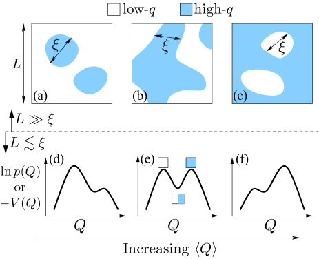
Figure 3: (a-c) Sketches of the spatial distribution of the overlap $q(\bm{r})$ within a large system ($L\gg\xi)$, as the average value of $Q$ increases. One expects a domain structure of high-$q$ and low-$q$ patches, with an associated length scale $\xi$, as indicated. (d-f) Sketches of distributions $\ln p(Q)=-N\beta V(Q)$ for small systems ($L\lesssim\xi$), under the same conditions as (a-c). For small systems then the domain structure leads to two peaks in $p(Q)$, with typical realisations of the system containing only one domain, as indicated in (e).

The key point is that if the situation in Fig. 3(a-c) holds in large systems, bimodal distributions $p(Q)$ will be found on considering finite systems of size $L\lesssim\xi$. The relevant distributions are sketched in Fig. 3(d-f), and are similar to those in Figs. 2(a,b). Our results are therefore consistent with the inactive state having a correlation length $\xi\gtrsim L$. This situation occurs in plaquette models at low temperatures jack-plaq-pin ; camma-patch , where the spacing between localised ‘excitations’ GC-2003 ; GC-annrev-2010 determines the range of amorphous order. It has also been proposed that a similar length scale determines the dynamical behaviour of non-equilibrium glass states formed by slow cooling keys2013 . Alternatively, the results of Fig. 2 are also consistent with the presence of a pinning-induced phase transition biroli-pin ; camma-pin-alpha ; berthier-kob-pin2013 , in which case $\xi$ would be infinite. In the absence of a finite-size scaling analysis, we cannot distinguish these two scenarios, so we simply conclude that $\xi\gtrsim L$ for the inactive states that we consider.

To reinforce the connection between large domains and the results of Fig. 2, it is useful to recall the implications of a non-convex effective potential $V(Q,c)$, which necessarily accompanies any bimodal distribution $p(Q|c)$. The potential is non-convex if, for some $Q$, $(\partial^{2}/\partial Q^{2})V(Q,c)<0$. Hence, there exist two values of the overlap $Q_{1},Q_{2}$ such that $V(Q_{1})+V(Q_{2})<2V(Q_{\rm ave})$, where $Q_{\rm ave}=\frac{1}{2}(Q_{1}+Q_{2})$. Therefore $p(Q_{1})p(Q_{2})>p(Q_{\rm ave})^{2}$. This means that systems which are globally high- or low-$q$ are more likely than systems where the domains are mixed, which implies that domain sizes $\xi$ are comparable with the system size $L$ camma-phase-sep . Note that this argument holds for finite systems, independently of the existence of any phase transition: it is the behaviour of $V(Q)$ as $N\to\infty$ that determines phase behavior berthier-silvio .

Finally, we note that fluctuations of the overlap in these systems come from several sources: the choice of the reference configuration and of which particles to pin (the fixed ‘template’), and the thermal fluctuations associated with the configuration $\mathcal{C}_{t}$. We find that the observed behaviour differs significantly between different realisations of the template: some templates are more likely to contribute to the large-$Q$ peaks in Fig. 2 while other templates contribute more to the small-$Q$ peak. In the picture of Fig. 3(a-c), this implies that the high- or low-$q$ regions of space are tied to specific locations in the system, depending on the structure of the template. However, on varying the choice of the frozen particles for a given reference configuration, we do not find any strong propensity for large-$Q$ or small-$Q$. That is, the specific reference configuration does not strongly influence where the large-$q$ or small-$q$ domains in Fig. 3 are located.

To conclude, the results presented here indicate that inactive non-equilibrium states from the $s$-ensemble have strong amorphous order, of a range $\xi$ comparable with the system size $L=5\sigma$. This order is much stronger that that found in equilibrium systems at the same temperature, consistent with the stability of the inactive states. The evidence for the large length scale $\xi$ is indirect, but Fig. 3 shows how bimodal overlap distributions can be attributed to the existence of large domains. More generally, these results show how dynamical (non-equilibrium) $s$-ensembles kcm-transition ; hedges09 can be combined with static concepts such as effective potentials franz-parisi-1997 and amorphous order BB-ktw-2004 ; montanari06 ; KL , in order to understand stable glassy materials.

We thank Juan Garrahan, David Chandler, Ludovic Berthier and Giulio Biroli for valuable discussions. This work was funded by the EPSRC through grant EP/I003797/1.

Appendix A Supplementary Information for “Investigating amorphous order in stable glasses by random pinning”

A.1 Model

In the Kob-Andersen mixture, particles of types $\alpha,\beta$ interact by a Lennard-Jones potential $V_{\alpha\beta}(r)=4\epsilon_{\alpha\beta}[(\sigma_{\alpha\beta}/r)^{1}2-(\sigma_{\alpha\beta}/r)^{6}]$, which is truncated and shifted at $r=2.5\sigma_{\alpha\beta}$ for numerical convenience. The particle types are labelled A and B and the interaction parameters are $(\sigma_{\rm AA},\sigma_{\rm AB},\sigma_{\rm BB})=(1.0,0.80,0.88)\sigma$ and $(\epsilon_{\rm AA},\epsilon_{\rm AB},\epsilon_{\rm BB})=(1.0,1.5,0.5)\epsilon$. We consider $N=150$ particles with $N_{\rm A}=(4N/5)$ and $N_{\rm B}=(N/5)$. The system is simulated by Monte Carlo dynamics berthier-mc2007 with a maximal step in each Cartesian direction of $0.075\sigma$, so the mean squared displacement for a single proposed move is $(0.075\sigma)^{2}$. Setting the time unit $\Delta t$ so that diffusion constant of a free particle is $D_{0}=\sigma^{2}/\Delta t$, one has the mean square displacement $\langle|\bm{r}(t)-\bm{r}(0)|^{2}\rangle=6D_{0}t=6\sigma^{2}(t/\Delta t)$. Letting $t$ be the time interval associated with a single MC sweep (one attempted move per particle), one sees that the time $\Delta t$ corresponds to $6/(0.075)^{2}\approx 1070$ MC sweeps.

A.2 Inactive configurations

The inactive configurations used in this work were obtained from an $s$-ensemble constructed as in Refs. hedges09 ; fullerton-veff . A trajectory $\bm{r}^{N}(t)$ of length $t_{\rm obs}=M\Delta t$, has activity $K[\bm{r}^{N}(t)]=\Delta t\sum_{i=1}^{N_{\rm A}}\sum_{j=0}^{M}|\bm{r}_{i}(t_{j})-\bm{r}_{i}(t_{j-1})|^{2}$, where $t_{j}=j\Delta t$. The corresponding “intensive” activity density is $k=K/(Nt_{\rm obs})$. A biased ensemble of trajectories $\bm{r}^{N}(t)$ is defined through $P_{s}[\bm{r}^{N}(t)]=P_{0}[\bm{r}^{N}(t)]\exp\{-sK[\bm{r}^{N}(t)]\}/{\cal Z}(s)$, where $s$ is a biasing field whose natural units are $(\sigma^{2}\Delta t)^{-1}$ and ${\cal Z}(s)$ is a normalisation constant. We use transition path sampling S (1) to sample these $s$-ensembles, as in hedges09 ; fullerton-veff .

In particular, we generated trajectories of length $t_{\rm obs}=400\Delta t$ with $s=0.015$ [in units of $(\sigma^{2}\Delta t)^{-1}$], as in fullerton-veff . The chosen value of $s$ corresponds to coexistence between the active and inactive phases, allowing efficient sampling of trajectories from the inactive phase. The inactive reference configurations that we use in this work were taken from trajectories in this $s$-ensemble: since the ensemble includes both dynamical phases, we take trajectories from the lower third of the activity distribution as being typical of the inactive phase. From these trajectories, the configurations at time $t_{\rm obs}/2$ form the set of configurations used as references: all results shown involve averages over a sample of $176$ independent configurations chosen in this way. Several templates were generated from each of these configurations, by independently choosing different sets of pinned particles.

A.3 Ensembles with pinned particles

Here, we give precise definitions of the ensembles that are associated with randomly pinned systems. This situation has been analysed in detail by Krakoviack krakoviack2010 but it is useful to review some results for the purposes of this work. Our notation here follows similar work for a spin model jack-plaq-pin .

Given a reference configuration $\mathcal{C}$ with particle positions $\bm{r}_{i}$, we define a binary variable $f_{i}=0,1$ for each particle, where $f_{i}=1$ means that particle $i$ is pinned, and $f_{i}=0$ means that it is free to move. Each $f_{i}$ is chosen independently, having the value $1$ with probability $c$ and $0$ with probability $1-c$.

Together, the reference configuration $\mathcal{C}$ and the variables $f_{i}$ encode the template, as described in the main text. Then, consider an ensemble of configurations $\mathcal{C}^{\prime}$ that are consistent with the template, with weights according to the Boltzmann distribution. That is, if the particle positions in $\mathcal{C}^{\prime}$ are $\bm{r}_{i}^{\prime}$ then

$$P(\mathcal{C}^{\prime}|\mathcal{C},\{f_{i}\})=\frac{1}{Z(\mathcal{C},\{f_{i}\})}\mathrm{e}^{-\beta E(\mathcal{C}^{\prime})}\prod_{j\in\cal F}\delta(\bm{r}_{j}^{\prime}-\bm{r}_{j})$$ (3)

where $E(\mathcal{C}^{\prime})$ is the energy of configuration $\mathcal{C}^{\prime}$, while $Z(\mathcal{C},\{f_{i}\})=\int\mathrm{d}\bm{r}^{\prime\prime N}\mathrm{e}^{-\beta E(\mathcal{C}^{\prime\prime})}\prod_{j\in\cal F}\delta(\bm{r}_{j}^{\prime\prime}-\bm{r}_{j})$ is a normalisation constant (partition function), and $\cal F$ is the set of particles $j$ with $f_{j}=1$. In some situations (for example a perturbative analysis at small-$c$ jack-plaq-pin ), it may be useful to write $\prod_{j\in\cal F}\delta(\bm{r}_{j}^{\prime}-\bm{r}_{j})=\prod_{j}[(1-f_{j})+f_{j}\delta(\bm{r}_{j}^{\prime}-\bm{r}_{j})]$ where the product on the right hand side now runs over all particles. This equality holds because the only possible values of $f_{j}$ are zero and unity.

In the dynamical simulations presented here, the Monte Carlo algorithm respects detailed balance with respect to the distribution (3), so on taking $t\to\infty$ for a given template, the configurations $\mathcal{C}_{t}$ generated by dynamical simulation must converge to the distribution of (3) with $\mathcal{C}^{\prime}=\mathcal{C}_{t}$. By sampling templates from a given distribution (equilibrium or inactive) and taking $t\to\infty$, one may therefore sample the joint distribution of $\mathcal{C}^{\prime}$ with the template. These joint distributions $P(\mathcal{C}^{\prime},\mathcal{C},\{f_{i}\})$ can be used to calculate the results of the main text: in particular, $p_{\rm eq}(Q|c)$ is the marginal distribution of $Q(\mathcal{C},\mathcal{C}^{\prime})$ obtained from a joint distribution $P(\mathcal{C}^{\prime},\mathcal{C},\{f_{i}\})$ that is formed by using (3) in conjunction with an equilibrated distribution for $\mathcal{C}$, and with $f_{i}$ chosen independently as described above. Similarly, $p_{\rm in}(Q|c)$ is a similar marginal but with $P(\mathcal{C}^{\prime},\mathcal{C},\{f_{i}\})$ constructed by drawing $\mathcal{C}$ from the inactive state.

For example, if $\mathcal{C}$ is chosen from an equilibrium state then the joint distribution of the template and the configuration $\mathcal{C}^{\prime}$ is

$$P_{\rm eq}(\mathcal{C}^{\prime},\mathcal{C},\{f_{i}\})=\frac{1}{Z_{f}}\mathrm{e}^{-\mu_{\rm f}\sum_{i}f_{i}}\\ \times\frac{1}{Z_{2}(\{f_{i}\})}\mathrm{e}^{-\beta E(\mathcal{C})-\beta E(\mathcal{C}^{\prime})}\prod_{j\in\cal F}\delta(\bm{r}_{j}^{\prime}-\bm{r}_{j})$$ (4)

where $Z_{f}=(1+\mathrm{e}^{-\mu_{\rm f}})^{N}$ and $Z_{2}(\{f_{i}\})=\int\mathrm{d}\bm{r}^{N}\mathrm{d}\bm{r}^{\prime N}\mathrm{e}^{-\beta E(\mathcal{C})-\beta E(\mathcal{C}^{\prime})}\prod_{j\in\cal F}\delta(\bm{r}_{j}-\bm{r}^{\prime}_{j})$.

For equilibrium pinning, we note that (4) is symmetric in $\mathcal{C}$ and $\mathcal{C}^{\prime}$, and the marginal distribution of $\mathcal{C}$ is the equilibrium distribution, by construction. Hence the distribution of $\mathcal{C}^{\prime}$ is also the equilibrium distribution of the system: that is, the structure of $\mathcal{C}^{\prime}$ is unaffected by the pinning. On the other hand, if $\mathcal{C}$ does not have an equilibrium distribution, as for the inactive reference states considered here, then the distribution of $\mathcal{C}^{\prime}$ is not equilibrated, nor is it equal to the distribution of $\mathcal{C}$. Rather, it represents a system that has biased away from equilibrium and towards to the inactive state, through the presence of the template.

References

- (1) M. D. Ediger, C. A. Angell and S. R. Nagel, J. Phys. Chem. 100, 13200 (1996).
- (2) P. G. Debenedetti and F. H. Stillinger, Nature 410, 259 (2001).
- (3) J.-P. Bouchaud and G. Biroli, J. Chem. Phys. 121, 7347 (2004).
- (4) A. Montanari and G. Semerjian, J. Stat. Phys. 125, 23 (2006).
- (5) J. Kurchan and D. Levine, J. Phys. A 44, 035001 (2011).
- (6) G. Adam and J. H. Gibbs, J. Chem. Phys. 43, 139 (1965).
- (7) T. R. Kirkpatrick, D. Thirumalai and P. G. Wolynes, Phys. Rev. A 40, 1045 (1989).
- (8) L. Berthier and W. Kob, Phys. Rev. E 85, 011102 (2012).
- (9) C. Cammarota and G. Biroli, Proc. Nat. Acad. Sci. USA 109, 8850 (2012).
- (10) W. Kob and L. Berthier, Phys. Rev. Lett. 110, 245702 (2013).
- (11) G. Biroli, J.-P. Bouchaud, A. Cavagna, T. S. Grigera and P. Verrocchio, Nature Physics 4, 771 (2008).
- (12) L. Berthier, Phys. Rev. E 88, 022313 (2013).
- (13) J. P. Garrahan and D. Chandler, Phys. Rev. Lett. 89, 035704 (2002); J. P. Garrahan and D. Chandler, Proc. Nat. Acad. Sci. USA 100, 9710 (2003).
- (14) D. Chandler and J. P. Garrahan, Ann. Rev. Phys. Chem. 61, 191 (2010).
- (15) J. P. Garrahan, R. L. Jack, V. Lecomte, E. Pitard, K. van Duijvendijk and F. van Wijland, Phys. Rev. Lett. 98, 195702 (2007); J. Phys. A 42, 075007 (2009).
- (16) L. O. Hedges, R. L. Jack, J. P. Garrahan and D. Chandler, Science 323, 1309 (2009).
- (17) R. L. Jack and J. P. Garrahan, Phys. Rev. E 81, 011111 (2010).
- (18) G. Biroli and J. P. Garrahan, J. Chem. Phys. 138, 12A301 (2013)
- (19) W. Kob and H. C. Andersen, Phys. Rev. E 51 4626 (1995); 52, 4134 (1995).
- (20) R. L. Jack, L. O. Hedges, J. P. Garrahan and D. Chandler, Phys. Rev. Lett. 107, 275702 (2011).
- (21) L. Berthier and W. Kob, J. Phys: Cond. Matt 19, 205130 (2007).
- (22) R. L. Jack and L. Berthier, Phys. Rev. E 85, 021120 (2012).
- (23) V. Krakoviack, Phys. Rev. E 82, 061501 (2010).
- (24) J. Kurzidim, D. Coslovich and G. Kahl, J. Phys.: Cond. Matt. 23, 234122 (2011).
- (25) K. Kim, K. Miyazaki and S. Saito, J. Phys.: Cond. Matt. 23, 234123 (2011).
- (26) S. Karmarkar and G. Parisi, Proc. Nat. Acad. Sci. USA 110, 2752 (2012).
- (27) B. Charbonneau, P. Charbonneau and G. Tarjus, Phys. Rev. Lett. 108, 035701 (2012).
- (28) R. L. Jack and C. J. Fullerton, Phys. Rev. E 88, 042304 (2013).
- (29) C. J. Fullerton and R. L. Jack, J. Chem. Phys. 138, 224506 (2013).
- (30) T. Speck, A. Malins and C. P. Royall, Phys. Rev. Lett. 109, 195703 (2012).
- (31) G. M. Hocky, T. E. Markland and D. R. Reichman, Phys. Rev. Lett. 108, 225506 (2012).
- (32) G. Szamel and E. Flenner, EPL 101, 66005 (2013).
- (33) S. Franz and G. Parisi, Phys. Rev. Lett. 79, 2486 (1997).
- (34) C. Cammarota, EPL 101, 56001 (2013).
- (35) R. L. Jack and J. P. Garrahan, J. Chem. Phys. 123, 164508 (2005)
- (36) C. Cammarota and G. Biroli, EPL 98, 36005 (2012).
- (37) See, for example, L. Berthier, G. Biroli, J.-P. Bouchaud and R. L. Jack, Ch. 2 in Dynamical Heterogeneities in glasses, colloids, and granular media, eds. L. Berthier, G. Biroli, J.-P. Bouchaud, L. Cipelletti and W. van Saarloos, (OUP, 2011).
- (38) A. S. Keys, J. P. Garrahan and D. Chandler, Proc. Acad. Nat. Sci. USA 110, 4482 (2013).
- (39) C. Cammarota, A. Cavagna, I. Giardina, G. Gradenigo, T. S. Grigera, G. Parisi and P. Verocchio, Phys. Rev. Lett. 105, 055703 (2010).

References

- S (1) P. Bolhuis, D. Chandler, C. Dellago, and P. Geissler, Ann. Rev. Phys. Chem. 53, 291 (2002).