Modes of asymmetry: the application of harmonic analysis to symmetric quantum dynamics and quantum reference frames
Abstract
Finding the consequences of symmetry for open system quantum dynamics is a problem with broad applications, including describing thermal relaxation, deriving quantum limits on the performance of amplifiers, and exploring quantum metrology in the presence of noise. The symmetry of the dynamics may reflect a symmetry of the fundamental laws of nature, a symmetry of a low-energy effective theory, or it may describe a practical restriction such as the lack of a reference frame. In this paper, we apply some tools of harmonic analysis together with ideas from quantum information theory to this problem. The central idea is to study the decomposition of quantum operations—in particular, states, measurements and channels—into different modes, which we call modes of asymmetry. Under symmetric processing, a given mode of the input is mapped to the corresponding mode of the output, implying that one can only generate a given output if the input contains all of the necessary modes. By defining monotones that quantify the asymmetry in a particular mode, we also derive quantitative constraints on the resources of asymmetry that are required to simulate a given asymmetric operation. We present applications of our results for deriving bounds on the probability of success in nondeterministic state transitions, such as quantum amplification, and a simplified formalism for studying the degradation of quantum reference frames.
I Introduction
Extracting non-trivial information about a system’s dynamics based on its symmetries is a standard technique in physics. Noether’s theorem is a prime example: it allows one to infer conservation laws from symmetries of closed-system dynamics. As it turns out however, for mixed quantum states, the Noether conservation laws do not capture all of the constraints on state transitions that arise from symmetries. Furthermore, for open-system dynamics, there are nontrivial constraints on state transitions arising from symmetries even though Noether’s theorem does not imply any MarvianSpekkensNoether .
The symmetry of a closed-system dynamics is simply the symmetry of the Hamiltonian that describes the dynamics. In an open-system dynamics, the system is not isolated but interacts with its environment. Then, if the total Hamiltonian of the system and environment respects a symmetry, and furthermore if the initial state of the environment also respects that symmetry then the effective evolution of the system will also have that symmetry.
Finding the set of all constraints on state transitions that are implied by symmetries of the dynamics (open or closed) is an important open problem. Solving it motivates the development of a general theory of the asymmetry properties of states, that is, the properties which describe the manner in which a state breaks symmetries, because these are the properties that determine the possibility of state transitions under symmetric dynamics.
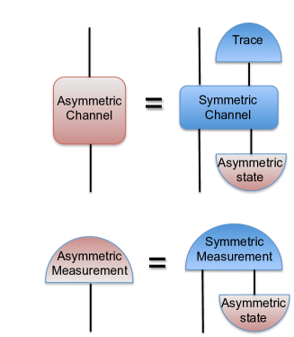
Developing such a theory is also important for the study of quantum references frames (see BRS07 for a review). In a context where the only experimental operations that can be freely implemented by an agent are symmetric, an asymmetric state becomes a resource because it can be used to simulate asymmetric channels and asymmetric measurements BRST06 ; BRST06b ; Poulin-Yard ; Sher-Bart ; Mar-Man ; BRST04 ; BIM ; Ahm-Rud ; MarvianSpekkensWAY (See Fig. 1). The restriction to symmetric operations can be understood as the result of lacking a reference frame, and an asymmetric state can be understood as a quantum token of the missing reference frame, allowing the agent to simulate measurements and transformations that are defined relative to the frame. So this provides another motivation for developing a general theory of asymmetry, one that characterizes not only the asymmetry properties of states, but of channels and measurements as well.
There has been significant progress towards this goal in recent years, in particular, on the asymmetry properties of pure states GS07 ; GMS09 ; MS11 ; MS11-Short ; thesis . For instance, Ref. MS11 provides a characterization of the equivalence classes of pure asymmetric states and the necessary and sufficient conditions for one pure state to be converted to another by symmetric processing for any symmetry corresponding to a compact Lie group. In the case of general mixed states, however, the problem is much harder and much less is known. Furthermore, there has been very little work on developing a unified framework for characterizing the asymmetry properties of quantum channels and measurements for arbitrary symmetry groups.
The theory of asymmetry also provides a framework for understanding quantum coherence as a resource. Coherence is considered in many cases to be the signature of quantum behaviour. Famous quantum phenomena such as the wave nature of particles, superconductivity, and superfluidity can all be interpreted as manifestations of quantum coherence. To understand the relation between asymmetry and coherence, consider the following example from quantum optics. Suppose is the state with photons in a given mode, and is the vacuum state. Consider the coherent superposition and the incoherent mixture . One way to understand the difference between these two states is that the coherent superposition is sensitive to phase shifts while the incoherent mixture is not. As such, coherence can be defined as asymmetry relative to phase shifts. This connection is explored further in Appendix A.
This article develops the theory of asymmetry by focusing on Fourier decompositions of quantum states, quantum measurements and quantum channels.
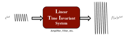
To give the flavour of our approach, we begin by recalling the significance of harmonic analysis (equivalently, Fourier analysis) for classical signal processing. If a processing is both linear and symmetric under time-translations (one says that the system is linear time invariant in this case), then one can decompose the input and output signals to different Fourier modes, i.e. different frequencies, such that a signal with frequency at the input can only generate a signal with the same frequency at the output (See Fig. 2).
We here consider an analogous decomposition of quantum states, measurements and channels into different modes. The key mathematical tool is the notion of irreducible tensor operators. Using these, one can develop a notion of a decomposition into modes for any symmetry described by a finite or compact Lie group. We refer to the modes appearing in such a decomposition as modes of asymmetry. Roughly speaking, different modes of asymmetry of a state (or measurement or channel) are different characteristic ways in which it can break a given symmetry. If for a given symmetry group, a state does not have a particular mode of asymmetry then under a symmetric dynamics it can never evolve to a state which has that mode of asymmetry. Similarly, it cannot be used as a quantum reference frame for simulating measurements or channels which have that mode of asymmetry. We also introduce some novel measures of asymmetry (i.e. asymmetry monotones) that can quantify the amount of asymmetry associated to a particular mode.
This approach provides us with a powerful tool for the study of asymmetry, one that is particularly well adapted to understanding asymmetric quantum states of finite-dimensional systems, i.e. quantum reference frames, as physical resources. For example, these tools allow one to determine which aspects of the quantum reference frame are relevant for the degree of success that can be achieved in a reference frame alignment protocol and more generally in covariant quantum estimation problems. Similarly, they allow one to determine which aspects of the quantum reference frame state are relevant for being able to simulate asymmetric channels or asymmetric measurements.
Previous work has sometimes identified, for certain tasks such as simulating measurements and channels, which properties of a quantum reference frame are relevant for performing that task, but these insights were achieved in an ad hoc manner and only for particular groups (See e.g. BRST06 ; BRST06b ; Poulin-Yard ; Sher-Bart ). The framework presented in this paper provides a unified and systematic way of determining what aspects of an asymmetric state are relevant for any such task, and it can also be applied to any finite or compact Lie group.
In the following we provide a couple of examples of results that one can derive with this framework.
I.1 Some examples of applications
I.1.1 Spin- system as quantum reference frame
Many authors have considered the example of a spin- system as a quantum reference frame for direction (See e.g. BRST04 ; BRST06b ; BRST06 ; BRS07 ; Poulin-Yard ; Mar-Man ; Sher-Bart ; BIM ; Ahm-Rud ; MarvianSpekkensWAY ). In particular, one interesting question which has been studied in several works is the problem of simulating measurements and channels that break rotational symmetry using rotationally-invariant interactions and the resource of a spin- system as a quantum reference frame.
For instance, Ref. Sher-Bart considers this problem for the special case of simulating channels and measurements on a spin- system using a spin- system as resource. To simplify the problem, it is assumed that the state of the spin- system is invariant under rotations around a direction , which is to say that it merely acts as a reference direction rather than as a full Cartesian frame. Using this assumption, Ref. Sher-Bart argues that the state of the quantum reference frame can be uniquely specified by real numbers corresponding to moments of , i.e. where is the state of the quantum reference frame and where is the angular momentum operator in the direction. This characterization is then used to quantify how well a given measurement or channel on a spin- system can be simulated.
As an example of the applications of our general results we reconsider this problem in section VI and we show how our approach leads to a great deal of simplification. In particular, we show that the quality of simulating a measurement (respectively a channel) on a spin- system only depends on (respectively ( and ). In other words, all the higher moments are irrelevant in this problem. More generally, we consider the problem of simulating measurements and channels on a spin- system instead of a spin-. In this case we show that the quality of simulating a measurement (respectively a channel) depends only on (respectively ) real parameters corresponding to the moments (respectively ).
Finally, we consider the general case where the spin- system does not have any symmetries, and hence can act as a full Cartesian frame. In theorem 23 we show that in this general case the quality of simulating a measurement (respectively a channel) is determined uniquely by the expectation value of all irreducible spherical tensor operators with rank less than or equal to (respectively ), i.e. by (respectively ) real parameters.
This example exhibits the power of the simple idea of mode decompositions of states, measurements and channels.
I.1.2 Bounds on Non-deterministic Amplifiers
An interesting application of the theory of asymmetry is to study the quantum noise generated by optical or electronic amplifiers. Such noise is inevitable in any amplification process and has a quantum origin. The traditional explanation is based on commutation relations in together with the linearity of the equations of motion Caves . But this approach cannot be applied to study the noise generated in non-linear amplifiers. Also, non-deterministic amplifiers, which were introduced in Ralph-Lund , fall outside the scope of applicability of this approach. A non-deterministic amplifier is defined as one that is allowed to only succeed with some nonzero probability (it must, however, produce a flag specifying whether it has succeeded or not), and this makes it possible to achieve amplification which produces less noise than would a deterministic amplifier, when it succeeds.
It turns out that the quantum noise generated in an optical amplification process can be explained as a consequence of a symmetry of the amplifier. This is the symmetry corresponding to the phase shifts of the input and output signals. So, a phase insensitive amplifier can be thought as an open-system dynamics with symmetry (amplification is necessarily an open-system dynamics because it requires a source of energy). Therefore, we can apply the general theory of asymmetry to find the consequences of symmetry in this open system dynamics. In particular, we can explain the origin of quantum noise in the following way: a symmetric dynamics cannot increase the amount of asymmetry. If a phase-insensitive amplifier did not generate noise and, for example, perfectly transformed a coherent state to another coherent state with larger amplitude, then the asymmetry of the output signal would be larger than the asymmetry of the input. This statement can be made quantitative using the notion of asymmetry monotones (see section II.1).
In this paper, we introduce a particular type of asymmetry monotone, one which quantifies the amount of asymmetry in a particular mode. Under a phase-insensitive amplifier, the amount of asymmetry in each mode is non-increasing. Therefore, for every mode of asymmetry, we get an independent constraint on the output signal. The advantage of this approach for explaining the origin of the noise is that it can be applied to a much broader range of amplification processes. In particular, it can be applied to nonlinear and non-deterministic amplifiers. In the following, we present an example of some results which can be obtained in this way.
Let be the number operator with eigenvectors such that . Here, the eigenvalue corresponds to the number of photons (excitations) in the input/output signals. This means that a phase shift is described by the unitary .
Consider a general input state described by the density operator . Suppose that under a phase-insensitive non-deterministic amplification process this state is transformed to with probability of success . Then, we show in section II.1 that the following inequalities hold
| (1) |
The th such inequality is a constraint derived from the non-increase of asymmetry in the th mode. In particular, these inequalities imply that if and are pure states and and then
| (2) |
To see an example of the consequences of these constraints, assume the input is a coherent state . There have been speculations that a nondeterministic quantum amplifier might be able to transform a coherent state to a coherent state for with a nonzero probability Ralph-Lund . Then, using Eq. (2) we find
| (3) |
In the limit , we can easily see that if , then the probability of transforming the coherent state to is zero. The conclusion that the probability of achieving a nontrivial amplification of a coherent state is strictly zero was also found in Refs. MenziesCroke and Amp13 by completely different arguments.
I.2 The structure of this paper
We begin by explaining the main ideas of the article using the simple example of a U(1)-symmetry associated with a (non-projective) unitary representation. Then we present the generalization to the case of arbitrary finite or compact Lie group with arbitrary projective representations. In the following we present an overview of the contents of the article.
In section II, we present the idea of a mode decomposition for the special case of the group U(1). In section II.1, we introduce asymmetry monotones which quantify the amount of asymmetry in each mode. Then in sections II.2 and II.3 we present some applications of the idea of mode decompositions in the context of phase references.
To generalize the concept of modes of asymmetry to arbitrary finite and compact Lie groups, we use the notion of irreducible tensor operators. We provide a short review of this subject in section III.1. In section III.2, we use this notion to introduce a representation of -covariant quantum operations, i.e., quantum operations which have symmetry relative to a unitary representation of group . This representation of -covariant operations basically characterizes them in terms of how they act on the irreducible tensor operators. We use this representation to define the notion of modes of asymmetry of states for arbitrary finite and compact Lie group in section IV, and we introduce the notion of asymmetry monotones that quantify the amount of asymmetry in a particular mode.
In section V.1, we generalize the idea of mode decompositions to quantum channels and measurements. The main motivation for this generalization is to study the problem of simulating quantum channels and measurements using quantum reference frames. This is done in section V.2 where we show how the mode decomposition of a quantum reference frame determines the measurements and channels which can be simulated by it. Finally, in Section VI, we apply these results to the important example of a spin- system as a directional quantum reference frame.
II Modes of asymmetry for the group U(1)
Let be an arbitrary unitary representation of the group . Let be an orthonormal basis in which the representation is decomposed into irreducible representations as
| (4) |
where the integer specifies the irrep of and is the multiplicity index.
Let be the space of linear operators on , which is clearly spanned by . Consider the subspace in spanned by operators . We denote this subspace by . We call any operator in this subspace a mode operator.
Suppose is a mode operator, i.e., it lives in . We may then write it as
| (5) |
It also follows that
| (6) |
On the other hand, if an operator satisfies Eq. (6) then by virtue of the linear independence of functions we can conclude that necessarily lives in the subspace . Therefore, we have
| (7) |
For an arbitrary operator , we can express it as a decomposition where . Here, is called the component of in mode . Note that for all we have . Furthermore
| (8) |
So to decompose a given operator to its modes we can use the following relation
| (9) |
Note that for any Hermitian operator it holds that .
Suppose is a U(1)-covariant super-operator, i.e.
Then, if both sides of this equation act on an arbitrary operator , we get
| (10) |
We can then infer from Eq. (7) that also lives in .
Note that this result did not require to be a completely positive map nor to be trace-preserving, but it certainly applies in these cases. We use the term quantum operation to refer to a completely-positive trace-nonincreasing superoperator, and quantum channel to refer to a deterministic (i.e. trace-preserving) quantum operation. We infer that U(1)-covariant quantum operations cannot change the mode of a state; they just map an operator in one mode to another operator in the same mode. In particular, if a U(1)-covariant channel maps state to then
| (11) |
where
| (12) | ||||
| (13) |
are the mode decompositions of and .
This suggests that we can interpret different as different modes of asymmetry: they cannot be interconverted to each other under U(1)-covariant quantum channels. In particular, if the initial state does not have a particular mode, then the final state of a U(1)-covariant dynamics also does not have that mode. (Of course, a mode can be eliminated if the associated component is mapped to zero by the dynamics.) Furthermore, a state is U(1)-invariant if and only if it contains only mode .
Let be the set of all integer ’s for which the state has a nonzero component in mode (This will always include ). So using this notation the above observation can be summarized as follows.
Proposition 1
Assume a state can be transformed to another state under a U(1)-covariant operation (deterministic or stochastic). Then
| (14) |
This proposition can be understood as a refined version of the simple fact that if the initial state of a U(1)-covariant operation is invariant under a U(1)-subgroup then the final state will also be invariant under that U(1)-subgroup. To see this, first recall that under the action of the symmetry group, state transforms as
| (15) |
Now suppose a state is invariant under the unitary for some integer such that . Using Eq. (15) and noting that the set are all linearly independent, we can conclude that for all modes which are not equal to an integer time , must be equal to zero. On the other hand, if for all ’s which are not equal to some integer times , then the state is invariant under . So, we conclude that uniquely specifies the symmetries of , i.e., all U(1)-subgroups which leave invariant.
Example 2
Consider a pure state . Let be the difference between the highest and lowest for which is nonzero. Then clearly, . Now proposition 1 implies that if there exists a U(1)-covariant channel which transforms a pure state to another pure state with a nonzero probability then . This implies that and therefore . This result has been obtained in Ref. GS07 using a totally different argument111The proof in Ref. GS07 proceeds by first finding a characterization of the Kraus operators of U(1)-covariant channels and then finding which pure state transformations are possible under quantum channels with this type of Kraus decomposition.. So the above proposition capture this result as a particular case.
We finish this section by providing a list of useful facts about modes of asymmetry:
1) Modes of asymmetry of a joint system: Suppose and are two states with the mode decompositions
We denote the mode decomposition of as . Then we can easily see that
| (16) |
2) Mode decomposition for a weighted twirling operation: Let be an arbitrary probability density and
| (17) |
Let
be the mode decomposition of and . Then
| (18) |
where is the th component of the Fourier transform of .
II.1 Quantifying the degree of U(1)-asymmetry in a given mode
Asymmetry monotones are functions from states to real numbers which quantify the amount of symmetry-breaking of any given state, such that the value of these functions are non-increasing under symmetric dynamics. The intuition is that since symmetric dynamics cannot generate asymmetry, any measure of asymmetry should be non-increasing under this type of dynamics. We take this as the defining property of asymmetry monotones. Introducing the notation to denote the fact that there exists a -covariant channel which transforms state to state , the definition is as follows BRST06 ; GS07 .
Definition 3
A function from states to real numbers is an asymmetry monotone if implies .
Recently several examples of asymmetry monotones have been proposed MarvianSpekkensNoether ; Vac-Wise-Jac ; GS07 ; Skot-Gour ; Tol-Gour-Sand ; GMS09 .
In this section, we consider the problem of quantifying the amount of asymmetry in each mode. In other words, we find asymmetry monotones which only measure the degree of asymmetry associated with some specific mode of asymmetry.
One family of such monotones can be constructed from the trace-norm. Recall that for an arbitrary operator the trace-norm of is . This norm is non-increasing under quantum channels (trace preserving, completely positive linear super-operators). So for any arbitrary quantum channel , we have
In the previous section we have seen that if is a U(1)-covariant channel which maps state to (with the mode decomposition ) then . Now the monotonicity of the trace-norm implies
So we can think of as a measure of the amount of asymmetry of the state in the mode .
Now suppose a given state can be transformed to another state under a U(1)-covariant channel with probability . If this is possible then there exists a U(1)-covariant channel which maps state to
where are two orthonormal states which are invariant under the symmetry transformations and is the completely mixed state on the Hilbert space of and is clearly invariant under all symmetry transformations. Now the fact that this channel is U(1)-covariant implies that for all : . However, because states and are invariant under the symmetry transformations this implies that for all it holds that
So to summarize, we have shown that
Proposition 4
Suppose there is a U(1)-covariant channel which maps a state to state with probability . Then it holds that
| (19) |
This proposition can be thought of as a quantitative version of proposition 1.
Using a similar argument, one can prove the following more general proposition about transforming a state to an ensemble of states.
Proposition 5
Suppose there is a U(1)-covariant channel that maps the state to the ensemble consisting of states with probabilities , where the value of becomes known at the end of the process. Then it holds that
| (20) |
This result subsumes proposition 4 as a special case because Eq. (20) implies that for any given value of ,
In the following, we calculate for arbitrary state in the case where the representation is multiplicity free, so that . (Note that all the previous results work for any representation of no matter if the representation has multiplicity or not.) Consider an arbitrary density operator . Then
Therefore
| (21) |
In particular, if the state is pure, i.e., where , then
| (22) |
Also, note that if the state is pure, then
| (23) |
where the bound follows from the Cauchy-Schwartz inequality.
It is also worth noting that the sum of this monotone over all modes, , is also an asymmetry monotone. It is equivalent to the asymmetry monotone presented in Eq. (44) of Ref. TolouiGour , with the equivalence manifest when the expression is worked out for pure states, in Eq. (49).
Example 6
Consider the sequence of states
| (24) |
One can easily see that for any given state there is a U(1)-covariant channel which transforms to a state arbitrary close to in the limit of large . is given by
| (25) |
The sufficiency of for forming approximations to any other state in the limit of large suggests that has the maximal possible asymmetry in this limit. This can be made precise as follows.
So for all modes for which , the state has almost the maximal value of asymmetry for mode with respect to this monotone (namely, the value 1, as shown in Eq. (23)).
II.2 Effect of misalignment of phase references
To be able to measure a quantity with high precision one fundamental requirement is to have a precise reference frame, for instance, in the case of measuring a time interval, a high precision clock. Any uncertainty in the configuration of the reference frame will limit the precision of the measurements that one can perform.
In this section, we consider the problem of misalignment of phase references. So we assume the system under consideration carries a non-trivial representation of the group U(1) given by . The U(1) group may have different physical interpretations: It may describe a rotation around some axis or a phase shift between states with different numbers of photons.
We assume there is an ideal perfect reference frame possessed by Alice and there is a noisy reference frame possessed by Bob. For example, Bob can be on a satellite and so has access to a clock with low accuracy while Alice is on earth and has access to a high precision atomic clock.
Assume they know that the phase shift relating Bob’s reference frame to Alice’s is with probability . If were known, then a state which is described by relative to Alice’s reference frame would be described by relative to Bob’s reference frame. Given that is only known to be distributed according to , it follows that the state is described relative to Bob’s reference frame as
| (26) |
which is generally a mixed state. This explains how the lack of a perfect reference frame can limit Bob’s ability to get information about an unknown state .
By Eq. (18), the state can be rewritten in terms of the mode decomposition of as
| (27) |
where is the th component of the mode decomposition of and
| (28) |
is the th component of the Fourier transform of .
So to understand how the uncertainty about the phase reference can affect Bob, it is helpful to consider the Fourier transform of the probability distribution . For example, if the Hilbert space of the system under consideration carries a finite number of irreps of U(1), then there will be a finite set of modes in which a state can have nonzero components. Then any quantity which quantifies the effect of misalignment described by the probability distribution should only depend on the Fourier component of in those particular modes.
II.2.1 Example
Consider the representation of U(1) given by where
Assume the phase difference between Alice and Bob’s local reference frames is with probability . Now, to quantify the effect of this misalignment on the description of an arbitrary state of this system we only need to consider the Fourier components of , denoted , for . For example, suppose Bob wants to estimate the phase of the state
| (29) |
The information about this phase lives only in the modes . So the only property of the probability distribution which is relevant for this estimation problem is its th Fourier component. In particular, if this component is zero, then Bob cannot get any information about the phase . This can happen even if the two phase references are highly correlated. For example, if
then has no component in the mode and therefore Bob cannot get any information about the phase . This simple observation shows that a measure of the alignment of two reference frames should be chosen based on the specific task to which the reference frames are being applied.
In many practical situations we can assume that the probability distribution is almost Gaussian. In particular, this is the case if Bob’s knowledge of is obtained by averaging over many independent estimations. Let be the standard deviation of . Then, for Gaussian distributions we know that for all modes with , and therefore for these modes the distribution is effectively a delta function over . So in the case of the above example where Bob is interested in estimating the phase of the state , if then the imperfectness of Bob’s local frame does not put any significant limitation on his performance.
II.3 Alignment of phase references using U(1)-asymmetric states
If Alice wishes to ensure that Bob’s reference frame is aligned with her own, she can send him a quantum reference frame, i.e., a quantum system prepared in an asymmetric state which carries information about her reference frame. For example, Alice can send Bob many copies of the state described by relative to her reference frame and also tell him the description of this state relative to her reference frame. Then Bob can use these quantum systems to obtain information about the relative phase between his reference frame and Alice’s.
Assume Alice and Bob’s prior knowledge about the phase difference between their local phase references is described by the probability distribution . Consider an arbitrary state described by relative to Alice’s reference frame. As we have seen before, the lack of information regarding the relation of Bob’s reference frame to Alice’s prevents him from obtaining as much information about the unknown state as Alice could. Now assume that Alice also sends Bob a quantum reference frame in the state and assume that the representation of phase shifts on this system is given by .
To find more precise information about , Bob can first use the quantum reference frame to align his reference frame with Alice’s and then perform some measurement on . But, this procedure does not describe the most general process that Bob can implement. The most general process is to perform a joint measurement on the state and the quantum reference frame . In this case the information Bob can obtain about the unknown state is the information he can extract from the state
| (30) |
This state is equal to
| (31) |
where is the mode decomposition of and is the th Fourier component of . This shows precisely how the information Bob can obtain about different modes of is determined by which modes are present in the state of the quantum reference frame and in the probability distribution decribing the misalignment.
II.3.1 Example
Suppose Alice and Bob’s local reference frames are initially uncorrelated and therefore the prior distribution is uniform.
Assume Bob wants to find information about the phase of the state
| (32) |
Note that here the information is encoded in the modes and . So to enable Bob to encode this information Alice should send him a quantum reference frame which has modes and . In particular, the reference frame should not be invariant under , because if then the state will not have any component in mode 2. But, lack of this symmetry does not imply that the quantum reference frame has mode 2. For example, assume Alice sends Bob the quantum reference frame
| (33) |
This state is not invariant under any subgroup of U(1). But it still does not have any component in the mode and so it does not help Bob to obtain information about the phase of the state (32).
III Representation of G-covariant channels in the irreducible tensor operator basis
In this section we first present a short review of irreducible tensor operators (See e.g. Cornwell and Sakuraii for more information on this subject.). Then, we introduce a new representation of G-covariant channels which basically describes a G-covariant channel by specifying how it acts on an irreducible tensor operator basis.
III.1 Review of irreducible tensor operators
Let be the space of all bounded operators acting on the Hilbert space . For any unitary the super-operator preserves the Hilbert-Schmidt inner product on , defined as for arbitrary . So the super-operator can be thought of as a unitary acting on the space .
Suppose is a projective unitary representation of a finite or compact Lie group on the Hilbert space . Then where is a unitary representation of on . Note that this representation is always non-projective,
| (34) |
Let be a basis of in which the representation decomposes to the irreps of such that
| (35) |
where
| (36) |
are the matrix elements of , the unitary (non-projective) irreducible representation of labeled by . We choose this basis to be normalized such that
| (37) |
Here, can be thought of as a multiplicity index. We call the basis the irreducible tensor operator basis. Also, the elements of the set for a fixed and are called components of the irreducible tensor . We call the irrep label the rank of the tensor operator .
Consider the Hermitian conjugate of both sides of Eq. (35),
| (38) |
where denotes the complex conjugate of . This implies that for any component of a tensor operator of rank , its Hermitian conjugate is in the subspace spanned by rank irreducible tensor operators where denotes the irrep equivalent to the complex conjugate of irrep . In particular, in the case of SO(3) (or equivalently SU(2)) where the complex conjugate of any irrep is equivalent to the irrep , the Hermitian conjugate of a component of an irreducible tensor operator with rank is in the subspace spanned by the irreducible tensor operators with rank .
To find an irreducible tensor operator basis in it is helpful to use the Liouville representation of operators in which an operator will be represented by a vector formed by stacking all the rows of its matrix representation (in some specific basis defining the representation) in a column vector Sher-Bart . This is equivalent to the Choi isomorphism between operators on and vectors on .
Then the Liouville (or Choi) representation of the super-operator will be where denotes the complex conjugate of in the basis that defines the representation. So the ranks of all tensor operators which show up in the space corresponds to the set of all irreps of which show up in the representation . Furthermore, to decompose a particular operator in to irreducible tensor operators we can write the Liuoville representation of that operator and find out how it decomposes into the irreducible basis of defined by the representation .
One can construct higher ranks of irreducible tensor operators by decomposing the product of irreducible tensor operators with lower ranks. Let be the components of a rank tensor operator and be the components of a rank tensor operator. Finally, let be the Clebsch-Gordon coefficients (see e.g. Sakuraii ). Then the set of operators defined by
| (39) |
are components of a rank irreducible tensor operator.
Finally, we present the Wigner-Eckart theorem which gives a useful tool to find the irreducible tensor operator basis (See e.g. Cornwell ):
Theorem 7
(Wigner-Eckart) Let be a finite group or a compact Lie group. Let be an element of a tensor operator. Then
| (40) |
where is a multiplicity index that counts the number of copies of the irrep that can be formed by composing irreps and , are the Clebsch-Gordon coefficients for this composition and is a number which is independent of , and .
Note that the left hand side of the equality can be interpreted as the matrix elements of the unitary acting on which transforms the orthonormal basis to the orthonormal basis .
Example: SO(3)
In the case of SO(3), the complex conjugate of any representation is unitarily equivalent to the original representation: Suppose is the complex conjugate of in the basis in which is diagonal and all the matrix elements of are real numbers. Then
| (41) |
Let be an arbitrary projective unitary representation of SO(3) on . The above discussion implies that one way to find the ranks of tensor operators and their multiplicities for the basis which spans is to find the irreps and their multiplicities which show up in the representation
An important special case, which we use later, is when carries a spin- irrep of SO(3). Then the above observation implies that is spanned by
and there is no multiplicity. In other words, the maximum rank of the irreducible tensor operators on this space is .
Note that the operators are uniquely defined only when we fix the basis we use to represent the matrix elements in Eq. (35). In the case of SO(3), we always use the basis in which the matrix representation of is diagonal and the matrix elements of are all real numbers.
Then, it follows that in this basis
where is the identity operator on , and are normalization factors Sakuraii .
One can generate all higher rank tensor operators on this space, by considering the products of and decomposing them to irreducible tensor operators using Eq. (39). Following this method one can show that the rank-2 irreducible tensor operators are
where is the total angular momentum and is a normalization factor (see e.g. Sakuraii ).
III.2 A representation of G-covariant super-operators
In this section, we introduce a representation of G-covariant super-operators which will be useful in the rest of this paper.
Recall that a super-operator is G-covariant if it commutes with the super-operator representation of the group G,
| (42) |
Then Schur’s lemma implies that should be block diagonal in any basis of the operator space which decomposes the representation into the irreps of . But, this is exactly the definition of an irreducible tensor operator basis and therefore -covariant channels are block diagonal in the irreducible tensor operator bases. The following lemma states this result.
Lemma 8
Let and be projective unitary representations of the group on the Hilbert spaces and . Let and be the corresponding normalized irreducible tensor operator bases for and . Consider a linear superoperator which is G-covariant, i.e., . Then
| (43) |
where (which turns out to be independent of ).
The proof is straightforward and is presented in appendix B. This representation simply means that under G-covariant super-operators, an input operator in the mode can only be mapped to an output operator in the same mode (for a general linear super-operator there is no such constraint on the output).
Lemma 8 implies that any linear G-covariant super-operator can be uniquely specified by specifying the set of matrices for the set of all which show up as ranks of irreducible tensor operators in both input and output spaces. In the next chapter we use this representation of G-covariant super-operators to study the asymmetry properties of quantum states. It can also have applications in other fields such as tomography of G-covariant channels or equivalently tomography of the symmetrized version of a channel (see Emerson1 ; Emerson2 ).
Example 9
Consider a rotationally covariant super-operator from to where the input and output spaces and are spin- and spin- irreps of SO(3) respectively.
Then, from section III.1 we know that the tensor operators for both input and output spaces do not have multiplicity and their rank varies between and in the input space and between and in the output space. So lemma 8 implies that an arbitrary rotationally covariant super-operator from to can be described by coefficients where varies between and
If this super-operator is a channel, i.e., it is trace-preserving and completely positive, then we can put more constraints on the coefficients . First, we use the fact that any completely positive super-operator maps Hermitian operators to Hermitian operators. This implies that all the coefficients should be real. On the other hand, the fact that a quantum channel is trace-preserving fixes one coefficient, namely, . So any SO(3) covariant channel on these spaces can be described by
real numbers. The special case of this result for has been observed previously in Sher-Bart .
In particular, if the input space is a spin-1/2 system, the channel can be described by just one real parameter. Note that in the absence of symmetry the number of parameters one needs to specify the channel scales as .
Let and be the irreducible tensor operator basis for and and be the coefficients describing the rotationally invariant super-operator from to . It follows from lemma 8 that if then
| (44) |
Finally, recall that the trace norm is non-increasing under positive and trace-preserving super-operators. This implies that if the super-operator is positive and trace-preserving then which by virtue of lemma 8 implies
| (45) |
In particular, if the input and output spaces are the same, i.e., , then
| (46) |
Consider the case where the output space of the G-covariant super-operator matches the input space of such that the composition is well-defined. If is described by the set of matrices and is described by the set of matrices then is described by the set of matrices . This implies that in cases such as the example above, where all tensor operators are multiplicity free and and are scalars, then all -covariant super-operators commute with each other. Furthermore, this observation implies that a master equation which describes a G-covariant dynamics can be decomposed to a set of uncoupled differential equations for each of these matrices.
IV Modes of asymmetry for an arbitrary group
With the framework of irreducible tensor operators in hand, we can now generalize the notion of modes of asymmetry, which we have thus far only defined for the case of U(1), to the case of arbitrary finite groups and compact Lie groups.
Consider the subspace spanned by for a fixed and . Then lemma 8 implies that any G-covariant super-operator maps an operator in this subspace to another operator in this subspace. This suggests the following definition of modes of asymmetry
Definition 10
The mode component of an operator , denoted , is defined by
| (47) |
We call the decomposition the mode decomposition of operator .
Note that in the above definition we have assumed that the basis is an orthonormal basis, i.e.
Lemma 8 has a simple interpretation in terms of mode decompositions of operators: a G-covariant super-operator maps an operator in a particular mode of asymmetry to an operator in the same mode of asymmetry, i.e., if then
| (48) |
So we can think of different pairs as different independent modes which cannot be mixed under a G-covariant linear super-operator. In particular, if an input has no component in a particular mode then the corresponding output also cannot have any component in that mode.
The above definition is independent of the choice of the tensor operators basis, . In the following lemma, we present another way to define modes of asymmetry which is explicitly basis independent.
Let be the (non-projective) set of all unitary irreps of a finite or compact Lie group and be the matrix elements of these unitary irreps. Recall that these matrix elements satisfy the orthonormality relations,
| (49) |
where in the case of finite groups the integral is replaced by the summation over all group elements. Then one can easily see that the following lemma holds.
Lemma 11
Let be the mode decomposition of operator . Then
| (50) |
where is the dimension of the irrep , is the uniform measure over the group and the bar represents complex conjugation.
Proof. We start with Eq. (35),
We multiply both sides by and integrate over . Now we use the orthonormality relations, Eq. (49). This implies that
| (51) |
The lemma follows from this equality together with the definition of mode decompositions given by Eq. (47).
This lemma gives us an alternative method to find the mode decomposition of a given operator.
It is worth emphasizing an important difference between the mode decomposition for the case of non-Abelian groups and the mode decomposition for the case of Abelian groups such as U(1). This difference concerns the result of symmetry transformations on operators in different modes. Since
| (52) |
it follows that modes and for which do not mix together under the action of the group, but modes for which and can mix together under this action. This can happen because in general a symmetry transformation is not a G-covariant operation, unless the group is Abelian. In the Abelian case, modes are just specified by an irrep label .
IV.1 Quantifying the degree of asymmetry in a given mode
As we saw in the specific case of the group U(1), one can quantify, for a given state, the amount of asymmetry in each mode in terms of the trace-norm of the component of the state in that particular mode. By a similar argument, it follows that for each mode the function defined by
| (53) |
is an asymmetry monotone.
The constraint on state to ensemble transformations, described in proposition 5 for the U(1) case, generalizes as follows:
Proposition 12
Suppose there is a G-covariant channel which maps the state to the ensemble containing states with probabilities where the value of becomes known at the end of the process. Then
| (54) |
Using definition 10 we can rewrite this bound as
As a simple corollary of proposition 12, if a nondeterministic G-covariant operation maps state to state with probability , then
| (55) |
IV.2 Example: spin- system
Consider the case of a spin- representation of SO(3). Then, as we have seen before, all the modes are multiplicity-free and so
Now, if a state of the spin- system evolves under a rotationally invariant dynamics to a state of the spin- system with probability , then for all modes it holds that
| (56) |
So, for example, in the case of mode , where for some constant we find
Note that here the direction is chosen arbitrarily and so for any direction it holds that
| (57) |
This result is very intuitive. If a spin- undergoes a deterministic or stochastic rotationally-covariant dynamics, the average of the absolute value of the expectation value of angular momentum can not increase. Note that the sign of this expectation value can change, i.e., a state whose angular momentum is negative in the direction can evolve to a state whose angular momentum is positive in this direction.
In this example we have assumed that the initial and final spaces are both spin- systems. On the other hand, one can easily show that the absolute value of angular momentum can increase if the final space is allowed to have a higher spin. In the following we will find a bound which applies to the cases where the initial and final spaces have different spins. Before this, we present another consequence of Eq. (56) for the case where both input and output spaces are spin-.
Although in a rotationally-covariant dynamics of a spin- system the absolute value of angular momentum cannot increase, nevertheless the expectation value of higher powers of angular momentum can increase. However, using Eq.(56), we can find non-increasing functions which involve the expectation value of higher powers of angular momentum. For instance, consider the case of . Then, as we have seen in section III.1, for a spin- representation of SO(3),
where is a normalization factor. Then Eq. (56) implies that
| (58) |
where we have used the fact that for all spin- systems the expectation value of is . Note that the direction is chosen arbitrarily. So, for arbitrary direction , is non-increasing under rotationally covariant dynamics, even though can increase.
Now we find a bound on the change of the absolute value of the expectation value of angular momentum when the input and output spaces have different spins.
To achieve this goal, we calculate for the mode in the case of a spin- system. Using the fact that for some constant , we find
| (59) |
where we have used the normalization condition, i.e. . One can easily see that and
| (60) |
So
| (61) |
So is less than or equal to 3/2 and at the limit of going to infinity it tends to .
Now we can find an analogue of the bound of Eq. (57) for the case where the input and output systems have spins and respectively. If, for example, both and are integer then
| (62) |
In proposition 21 below, we show that the quantity admits of an operational interpretation: it quantifies the ability of the state to act as a quantum reference frame for the task of distinguishing, on a spin-1/2 system, the two eigenstates of , and .
V Simulating quantum operations by quantum reference frames
Consider the situation where we are restricted to those Hamiltonians which all have a particular symmetry. Then it is still possible to simulate a dynamics which breaks this symmetry if we have access to a state which breaks the symmetry, i.e. a source of asymmetry. As we have mentioned earlier, this symmetry-breaking state is called a quantum reference frame. By coupling this quantum reference frame to a system via a symmetric dynamics, we can effectively generate an asymmetric dynamics or measurement on this system. In this section we are interested in finding the set of asymmetric dynamics and measurements which can be simulated using a given quantum reference frame.
As a simple example, consider the case where we are restricted to the rotationally-invariant Hamiltonians. Then by coupling a quantum system to a large magnet with magnetic field in the direction via a rotationally invariant Hamiltonian, we can effectively simulate a rotation around the axis on that quantum system (note that a rotation is not a rotationally invariant operation and so cannot be performed without having access to a system which breaks the rotational symmetry). In this case, we can model the magnet by a spin- system in a large coherent state polarized in the direction, i.e., in the maximum weight eigenstate of , . Then, by coupling the quantum system to this quantum reference frame one can realize a quantum channel on the system such that this channel at the limit where goes to infinity approaches a perfect (unitary) rotation. In fact, one can show that using a spin- in the coherent state in direction, at the limit of large any arbitrary dynamics which is invariant under rotation around can be simulated on the system Mar-Man .222Furthermore, it is shown in Ref. Mar-Man that if in addition one has access to a similar quantum reference frame in a coherent state polarized in the direction then one can simulate arbitrary dynamics on the system.
Note that by having access to this quantum reference frame we still cannot simulate a rotation around or any other dynamics which is not invariant under rotation around . More generally, for a given quantum reference frame, only those time evolutions and measurements can be simulated which have all the symmetries of the quantum reference frame. In this section we generalize this simple observation by finding a relation between the modes of asymmetry of the quantum reference frame and the modes of asymmetry of a time evolution or measurement that can be simulated using it.
V.1 Modes of asymmetry of quantum operations
The notion of modes of asymmetry naturally extends to the super-operators. Let be the projective unitary representation of on the Hilbert space . Also, let . Then is a (non-projective) unitary representation of on . Similarly, we can define a representation of on the space of all linear super-operators: Consider the linear space of all super-operators from to . Then a natural representation of on this space is given by the following map
| (63) |
for arbitrary , where and are the representations of the symmetry on and respectively. This representation has a natural physical interpretation: suppose the representation describes a change of reference frame, such that a state which is described by in the old reference frame is described by in the new reference frame. Then, an observable or a density operator which is described by an operator relative to the old reference frame will be described by relative to the new reference frame. Similarly, a super-operator which is described by relative to the old reference frame will be described by relative to the new reference frame.
Now, following the same logic we used to define modes of asymmetry of operators based on the representation of group on the space of operators, we can define the notion of modes of asymmetry of super-operators based on the representation of group on the space of super-operators. One way to do this is by defining the analogues of the irreducible tensor operators for super-operators. Alternatively, we can define modes of asymmetry for super-operators using the analogue of lemma 11:
Definition 13
The mode of the super-operator , denoted by is defined by
| (64) |
where is the dimension of the irrep . We call the decomposition the mode decomposition of the super-operator and the modal component of .
Note that this definition implies that a G-covariant super-operator only has nonzero component in the mode which corresponds to the trivial representation of the group, denoted by .
Let be the representation of the symmetry group on the Hilbert space . As we have seen before, we can find the set of all modes of asymmetry that an operator can possibly have, by decomposing the representation . Similarly, we can find all modes of asymmetry that a super-operator can possibly have, by decomposing the representation
to irreps of . Here, and are the representations of the symmetry group on and respectively.
Example 14
Consider the group of rotations in , i.e. G=SO(3), and assume the input Hilbert space carries a irrep and the output Hilbert space carries a irrep. Then any super-operator from to can have modes with . In particular, if the input and output spaces of a super-operator are both spin-1/2 systems (i.e. ), then the super-operator can only have modes and . On the other hand, if the input space is a spin-1/2 irrep of SO(3) and the output space is invariant under rotation (i.e. and ) then the super-operator can only have modes . These latter kind of super-operators can describe, for example, measurements on a spin-1/2 system where the post-measurement state is always rotationally invariant.
In this example, we found all modes of asymmetry that a measurement performed on a spin-1/2 system can possibly have. In the following we study the notion of modes of asymmetry of measurements more closely.
V.1.1 Modes of asymmetry of measurements
In the study of the modes of asymmetry of measurements, we focus on the aspect of a measurement that is relevant for making inferences about the input, that is, its informative aspect, and neglect the aspect that is relevant for making predictions about future measurements on the system, that is, its state-updating aspect.
Let be the POVM describing an arbitrary measurement. Define the channel
| (65) |
where the set consists of orthogonal and G-invariant states. Then, any measurement whose statistics is described by the POVM can be realized by first applying the channel to the state and then measuring the output system in the basis. But, this latter measurement is G-covariant and so one does not need a quantum reference frame to realize it. So to find the asymmetry resources required to implement a measurement of the POVM , it suffices to find the asymmetry resources required to implement .
One can easily show that
Lemma 15
, the modal component of , is equal to
| (66) |
where is the modal component of the operator .
Proof. First note that by definition 13,
| (67) |
Here, the representation of symmetry on the output system is trivial and so
Further on, we will use this observation to infer the asymmetry resources which are required to implement a given measurement.
V.2 From modes of quantum reference frames to modes of quantum channels
As described above, under the assumption that all symmetric dynamics are free we can use a quantum reference frame, which breaks the symmetry, as a resource of asymmetry which enables us to simulate dynamics which break the symmetry.
Definition 16
Let and be Hilbert spaces with projective unitary representations and of group . We say that a channel can be simulated using the resource state if there exists a channel which is G-covariant, i.e.,
such that
| (68) |
Now one can easily prove the following result.
Lemma 17
Suppose the channel can be simulated using a quantum reference frame in the state and a G-covariant channel such that . Then
| (69) |
Proof. First, note that
Then, because is G-covariant, we have
By multiplying both sides by and taking the integral over , we prove the lemma.
In the previous section, we defined to be the set of all modes in which state has nonzero components. Similarly, we define to be the set of all modes in which a channel has nonzero components. Then the above lemma implies that
Proposition 18
If a quantum reference frame can simulate a quantum channel then
| (70) |
So if a quantum reference frame does not have a particular mode of asymmetry, it cannot simulate a time evolution or measurement which has that mode of asymmetry. Also, the lemma implies that to specify whether a given quantum reference frame can simulate a quantum channel or not we only need to know the components of in modes contained in . So, as we will see in an example, although the Hilbert space of the quantum reference frame might be arbitrary large, the number of parameters required to specify its performance for some specific simulation can be very small.
Furthermore, for any given finite dimensional Hilbert space , there are a finite set of modes in which a channel acting on can have nonzero components. So for a given quantum reference frame on an arbitrarily large Hilbert space and having amplitude over arbitrarily many representations of the group, the properties of the quantum reference frame which are relevant for simulating arbitrary channels acting on can be specified merely by specifying the components of in that finite set of modes.
Example: Reference frames of unbounded size may still lack modes
In the case of =SO(3), consider the family of quantum reference frames defined by
One can easily show that, at the limit of large these states are very sensitive to rotations around and also rotations around any axis in the plane. In other words, for any small such rotation, is almost orthogonal to the rotated version of . So, one may think that at the limit of large this quantum reference frame completely breaks the symmetry and so it can be used to simulate any arbitrary measurement on a spin-1/2 system. This is not the case, however. Indeed, it turns out that even though at the limit of large these states are very sensitive to rotations around (that is, they break this symmetry), nonetheless they cannot simulate any measurement on a spin-1/2 system which is not invariant under rotations around . To see this, first note that if the POVM elements of a measurement on a spin-1/2 system are not invariant under rotations around then they have nonzero components in the modes . Then, lemma 15 implies that the channel describing that measurement will have modes . Now proposition 18 implies that to be able to simulate any such measurement a quantum reference frame needs to have a non-zero component in the modes . However, using the Wigner-Eckart theorem, one can easily show that none of the states in the above family have a nonzero-component in the modes 333Consider the terms in the decomposition Any term in this decomposition with is invariant under rotations around and so it only has components in modes . On the other hand, terms with have no components in any of the modes because and always differ by at least 2. .
The conclusion is that there are measurements that break rotational symmetry that cannot be simulated by this family of quantum reference frames.
VI Example: Spin- system as a quantum reference frame
The problem of using a spin- system as a quantum reference frame to simulate dynamics or measurements which are not invariant under rotations has been studied in several papers (See e.g. BRST04 ; BRST06b ; BRST06 ; BRS07 ; Poulin-Yard ; Mar-Man ; Sher-Bart ; BIM ; Ahm-Rud ; MarvianSpekkensWAY ). In this section, we show that the mode decomposition of states provides an extremely powerful insight into this problem. In particular, we show that using this approach some of the previously known results which have been achieved in an ad hoc manner can be reproduced and generalized in a systematic way.
VI.1 Simulating measurements and dynamics on a spin-1/2 system
We start with the problem of simulating measurements on a spin-1/2 system. Here, the assumption is that we are restricted to use rotationally-invariant unitaries, ancillary systems in rotationally-invariant states and measurements whose POVM elements are all rotationally-invariant. Under this restriction, we are given a spin- system in an arbitrary state as a quantum reference frame and our goal is to simulate a non-invariant measurement on a spin-1/2 system. Here, we focus on the informative aspect of the measurement, that is, we are not concerned with how the state of system is updated after the simulated measurement.
For an arbitrary measurement on a spin-1/2 system, consider the channel which describes the informative aspects of this measurement, as defined in Eq. (65). Then, consider the set of all modes in which this channel can have nonzero components. We can conclude from lemma 15 that this set is equal to (This is also shown in example 14.).
Then, it follows from proposition 17 that the only properties of that are relevant for its performance in simulating a measurement on a spin-1/2 system are its components in the modes , i.e., and . Furthermore, since the irreducible tensor operator basis on a spin- system is multiplicity-free, each of these components is determined by only one parameter, namely, the Hilbert Schmidt inner product between and the corresponding component of the irreducible tensor operator basis,
where and are normalization factors. It follows that the components of in the modes are uniquely specified by the vector of expectation values of angular momentum for , i.e.,
So we conclude that
Proposition 19
Consider a spin- system in state as a quantum reference frame. Its performance in simulating (informative aspects of) measurements on a spin-1/2 system is uniquely specified by the vector of expectation values of angular momentum of .
This result has been previously obtained in Poulin-Yard using a totally different and rather ad hoc argument. But, using our approach we can easily generalize it to the case of measurements on systems supporting arbitrary representations of SO(3) (as opposed to just the spin-1/2 representation). Before presenting this generalization we investigate some implications of proposition 19.
An interesting consequence is the following: Suppose the system is spin- and the vector of expectation values of angular momentum of is polarized in the direction. In general, for , such a state need not be invariant under rotations around . Now consider the symmetrized version of , i.e., the state
which is invariant under rotations around . One can easily see that this state has the same vector of expectation values of angular momentum as the original state . Therefore, any measurement on the spin-1/2 system which can be simulated using can also be simulated using and vice versa. But, since is invariant under rotations around , it can only simulate those measurements whose POVM elements are invariant under rotations around . This argument implies that
Corollary 20
Consider a spin- system in state as a quantum reference frame for direction. If has a vector of expectation values of angular momentum that is polarized in the direction, then it can only simulate those measurements on a spin-1/2 system for which the POVM elements are invariant under rotations around .
So, even at the limit of large , a single spin- system cannot act as a perfect reference frame for direction even if it does not have any symmetries.
As an example of simulating measurements on a spin-1/2 system consider the following problem: suppose one uses a spin- system in the state as a quantum reference frame to measure the angular momentum of a spin-1/2 system in the direction, that is, to measure the observable . It can be shown that this measurement cannot be simulated perfectly with a quantum reference frame of bounded size. This result is known as the Wigner-Araki-Yanase theorem Wigner ; ArakiYanase ; LoveridgeBusch , and is quite an intuitive result in the context of the resource theory of asymmetry MarvianSpekkensWAY ; Ahm-Rud . Now the question is: using the spin- system in the state as a quantum reference frame, how well can one simulate this measurement? In other words, using this quantum reference frame, what is the highest precision attainable in a simulation of a measurement of ? We evaluate the precision of the realized measurement using the following figure of merit: the highest probability of successfully distinguishing an unknown eigenstate of when we are given each of the two eigenstates with equal probability.
The answer, which we prove in the appendix, is as follows.
Proposition 21
Suppose we are restricted to the rotationally invariant measurements but we have access to the state of a spin- system as a quantum reference frame. Then the maximum probability of successfully distinguishing the two eigenstates of for a spin-1/2 system, and , when the prior probabilities of the two are equal, is given by
| (71) |
So, as we expected from proposition 19, this probability only depends on the expectation value of the vector of angular momentum (in this case, just the component). Note that, as one may expect intuitively, in the limit where becomes arbitrarily large, the coherent state can be used as a quantum reference frame to simulate the measurement of perfectly.
Finally, it is worth mentioning that if the Hilbert space of the quantum reference frame under consideration carries different irreps of SO(3) or if it has more than one copy of an irrep, then the vector of angular momentum of the reference frame state alone is not sufficient to specify the measurements it can simulate on a spin-1/2 system. For example, suppose the quantum reference frame is formed from a spin- system and a qubit whose states are invariant under rotation. This means that the total Hilbert space of the quantum reference frame has two copies of irrep of SO(3). Suppose the quantum reference frame is in the state
where labels different orthogonal states of the qubit. Then, one can easily show that at the limit of large this reference frame can simulate any arbitrary measurement which is invariant under rotation around . But, the expectation value of angular momentum for this state is zero in all directions. So, for a general representation of SO(3) these expectation values cannot characterize the ability of the state to simulate measurements on a spin-1/2 system.
Proposition 19 can be easily generalized to the problem of simulating arbitrary dynamics on a spin-1/2 system.444This includes, as a special case, the problem of simulating measurements when we are concerned with simulating not just their informative aspect, but the particular update rule as well.
Recalling example 14, it is clear that the modes of asymmetry appearing in the modal decomposition of a channel on a spin-1/2 system are . So, proposition 17 implies that to specify the ability of a particular state of the spin- system to simulate an arbitrary dynamics on a spin-1/2 system, we merely need to specify these modes of asymmetry of . Again from the result of section III.1 we can see that the components of in these modes are uniquely specified by the following eight real parameters:
| (72) |
So to summarize we have shown that
Proposition 22
Consider a spin- system in state as a quantum reference frame. Its performance in simulating channels on a spin-1/2 system is uniquely specified by the eight real parameters specified in Eq.(VI.1).
VI.2 Generalization to arbitrary systems
In the previous section we considered the problem of simulating measurements and channels on spin-1/2 systems. In this section we generalize these results to arbitrary systems. We start by a generalization of propositions 19 and 22.
Theorem 23
Consider a spin- system in state as a quantum reference frame. Its performance for simulating a measurement (respectively channel) on a system with Hilbert space is uniquely specified by (respectively ) real parameters, where is the largest angular momentum quantum number which shows up in the decomposition of into irreps of SO(3). These parameters of correspond to the expectation values of all the non-trivial irreducible tensor operators with rank less than or equal to (respectively ).
The proof is presented in appendix B. Note that an arbitrary state of a spin- system is specified by real parameters. But the above result implies that the number of parameters of that are relevant for its performance in the simulation task depends only on , the size of the system to which the measurement or channel is applied, and not on , the size of the quantum reference frame.
An important special case is where the state is invariant under rotations around some axis . This special case has been previousy considered for example in Sher-Bart . It follows from theorem 23 that
Corollary 24
Consider a spin- system in state as a quantum reference frame, and suppose that is invariant under rotations around the direction . Its performance in simulating a measurement (respectively channel) can be uniquely specified by (respectively ) real parameters corresponding to the moments (respectively ) where is the angular momentum operator in the direction.
Note that to specify an arbitrary state of a spin- system which has the relevant symmetry property (invariance under rotations around direction ), one needs real parameters. An instance of these parameters are . This particular characterization of states is used in Sher-Bart to specify how the quality of a quantum reference frame degrades after using it to simulate a channel or measurement.
In particular, they use this characterization to study the problem of simulating channels on a spin-1/2 system and of simulating measurements on a spin-1 system. But from the result of corollary 24 we know that to specify the performance of the quantum reference frame in both of these cases, we only need to specify two real parameters, namely, and . As we will see next, this can lead to a significant simplification of the problem of characterizing how a quantum reference frame degrades when used to implement measurements and channels on another system.
VI.3 Degradation of quantum reference frames
Using a quantum reference frame to simulate a symmetry-breaking measurement or channel will inevitably degrade it. This degradation of quantum reference frames can be understood as a manifestation of the fact that obtaining information about a quantum system will necessarily disturb it.
For example, in the case of rotational symmetry, consider a quantum reference frame which specifies an unknown direction in space. We can use this quantum reference frame to simulate a rotation around this unknown direction on an object system. But by comparing the initial and final state of the object system we can obtain some information about the unknown direction. So, using a quantum reference frame for simulating a rotation can be understood as performing a measurement on the quantum reference frame and since we thereby obtain some information about the quantum reference frame, its state is necessarily disturbed in the process.
Different aspects of the degradation of quantum reference frames have been studied in several papers (See e.g. Aha-Kauf ; Aha-Popes ; BRST06 ; BRST06b ; Poulin-Yard ; Sher-Bart ; Ahm-Rud ; MarvianSpekkensWAY and the references in BRS07 ). A central question studied in these papers is how the performance of the quantum reference frame for simulating the measurement or channel drops as a function of the number of implementations of the latter.
A natural special case of the degradation problem, considered in BRST06 ; BRST06b ; Sher-Bart , is where the average of the state of the system to which the measurement or channel is applied is symmetric. In other words, each time we use the quantum reference frame to simulate an operation on the object system, the initial state of the object system is chosen at random from an ensemble the average state of which does not break the symmetry. So, for example, in the case of rotational symmetry, which we study in this section, the average state of the object system is assumed to be rotationally-invariant.
Then it follows that under this assumption the degradation of the quantum reference frame will be described by a rotationally-covariant channel. In other words, the state of the quantum reference frame after uses, denoted , will be
| (73) |
where is a G-covariant channel. This implies that under this assumption about the distribution of the states of the object system, different modes of asymmetry of the quantum reference frame degrade independently, i.e.,
| (74) |
This simple observation can greatly simplify the analysis.
Consider the case of spin- quantum reference frames for direction. First, note that this observation together with theorem 23 implies that the quality of simulation of a channel or measurement on an object system after using the quantum reference frame for arbitrary number of times only depends on a fixed number of parameters of the initial state of the quantum reference frame and this number is independent of the size of the quantum reference frame.
Furthermore, from example 9 we know that since the channel which describes the degradation of the quantum reference frame is rotationally covariant it holds that
| (75) |
where is a set of real coefficients which describe the channel and . But since, for a spin- representation of SO(3), the elements of the irreducible tensor operator basis are multiplicity-free it holds that and therefore
| (76) |
So if and are respectively the initial state of the quantum reference frame and its state after uses, then it holds that
| (77) |
Since we can conclude that each of the modal components of the state of the quantum reference frame either remains constant or decays exponentially.
Example 25
Here, we consider the scenarios studied in Sher-Bart where a spin- system is used as a quantum reference frame to simulate channels on a spin-1/2 system and measurements on a spin-one system. Furthermore, it is also assumed that the average of the state of the object system is rotationally-invariant. This implies that the channel which describes the degradation of the quantum reference frame is also rotationally-covariant. It is also assumed in Sher-Bart that the state of the quantum reference frame is initially invariant under rotation around an arbitrary direction which we denote by . Note that since the degradation of the quantum reference frame is described by a rotationally-covariant channel, the state of the quantum reference frame will remain invariant under rotations around .
Now from theorem 23 and corollary 24 we know that the performance of the state of this quantum reference frame for these simulations is uniquely specified by two real parameters: the components of in modes and . But these are specified by
where and are independent of .555 and . Note that since the state by assumption is confined to the irrep of SO(3), it follows that and so
In other words, the quality of simulation is uniquely specified by the expectation values of the first and the second moments of for .
Now using Eq. (77) we can conclude that if the initial state of the quantum reference frame is and if we have used the quantum reference frame times then the quality of the th simulation is uniquely specified by
| (78) |
and
| (79) |
where is the set of coefficients which describe the degradation channel . So, in the example studied in Sher-Bart , the only properties of the channel which are relevant to specify the drop in the quality of simulation after many uses are the two real coefficients and . Finally, note that since then Eq.(78) implies that the absolute value of is either constant or decays exponentially with . Similarly, since then Eq.(79) implies that is either constant or exponentially saturates to , which is the expectation value of for the completely mixed state.
VII Acknowledgements
We acknowledge helpful discussions with Gilad Gour. Also, RWS acknowledges an early discussion with Matthias Christandl on the topic of simulating channels with quantum reference frames. Research at Perimeter Institute is supported in part by the Government of Canada through NSERC and by the Province of Ontario through MRI. IM acknowledges support from NSERC, a Mike and Ophelia Lazaridis fellowship, and ARO MURI grant W911NF-11-1-0268.
Appendix A Quantum coherence as asymmetry relative to phase shifts
We here argue that quantum coherence, considered as a resource, is simply the resource of asymmetry relative to phase shifts.
Consider the case of coherence between the eigenspaces of a number operator . For the phase complementary to , the group of phase shifts is represented by the set of unitaries . Clearly, the set of states that are invariant under phase shifts are those that are block-diagonal relative to the eigenspaces of the number operator, i.e., precisely those that have no coherence relative to these eigensapces. Hence, a state with coherence is one that has some asymmetry relative to phase shifts.
Another observation which supports this view of coherence is that phase-insensitive operations, that is, operations that commute with all phase shifts, cannot generate coherence. In other words, under a phase-insensitive time evolution, incoherent states such as or cannot evolve to states which have coherence. From the point of view of the theory of asymmetry, this is a special example of the more general fact that for any given symmetry, symmetric time evolutions cannot take symmetric states to asymmetric states. Therefore, the problem of quantifying and classifying coherence can be considered as a special case of the theory of asymmetry where the group under consideration is U(1). The theory of asymmetry is more general, however, because it also concerns non-Abelian groups, such as SO(3), where there is no preferred set of subspaces coherences between which imply asymmetry.
A slightly different approach to the study of coherence was recently proposed in Plenio . Instead of focusing on phase-insensitive operations, the focus is on a class of incoherent operations, which is defined as the set of all operations that transform every incoherent state to another incoherent state. One can easily show that incoherent operations are a proper subset of phase-insensitive operations: For instance, for any and , the transformation can be realized via an incoherent operation while it is forbidden under phase-insensitive operations unless . In other words, incoherent operations allow arbitrary permutations among the number eigenspaces. It follows that all states of the form for are equivalent (i.e. reversibly interconvertable) under incoherent operations, whereas they are not all equivalent relative to phase-insenstive operations.
To decide which of these two subsets of quantum operations is best suited to define coherence as a resource, one should consider whether there is some realistic restriction on experimental capabilities that would imply the realizability of only this subset. In other words, we ask whether one can provide an operational interpretation of either subset. Just an interpretations exists for phase-insensitive operations: these arise from the restriction that is imposed on a pair of parties when they lack a shared phase reference BRS07 . For instance, if the phase describes the configuration of an oscilator that is acting as a clock, then if two parties fail to have synchronized clocks, they lack a shared phase reference. In these situations the transformation cannot happen unless . On the other hand, it is not clear if there is any operational scenario which motivates the study of incoherent operations.
This analysis is bolstered by considering a similar distinction in entanglement theory. The subset of quantum operations that is taken to define the resource of entanglement is the set of Local Operations and Classical Communication (LOCC). This is distinct from the set of non-entangling operations, the operations which map unentangled states to unentangled states. The latter set in particular includes nonlocal operations such as swapping two separated systems. There is no obvious restricton on experimental capabilities that would permit swapping without also permiting the use of a quantum channel. In other words, while the set of LOCC operations has a clear operational meaning, the set of nonentangling operations does not. Nonlocal operations such as swap are the counterpart, within the set of nonentangling operations, of the general permutations within the set of incoherent operations: neither seems to admit of a good operational interpretation.
Appendix B Proofs
B.1 Proof of lemma 8
Since is a basis for then for any map
| (80) |
for some coefficients . Now we apply the super-operator to both sides of the above equation. Applying on the left hand side and using G-covariance of we get
| (81) |
On the other hand, applying to the right-hand side of Eq.(80) we get
Equating the right hand sides of the above two equations and using the orthogonality of the functions we find that can be written as
| (82) |
So we conclude that
| (83) |
Note that the orthonormality of the basis implies
| (84) |
which holds for all . Finally, we notice that the orthonormality of the basis together with linearity of implies
| (85) |
These last three equations together prove the lemma.
B.2 Proof of Theorem 23
We start by the proof in the case of measurements. This proof follows exactly the same as the proof in the special case of spin-1/2 systems. Suppose is the Hilbert space of the system on which we simulate the measurement. Then by assumption the largest irrep of SO(3) showing up in is . Let denote the projective representation of SO(3) on .
Then, as we have seen in section III.1 the set of possible ranks of the irreducible tensor operators acting on is the same as the set of all irreps of SO(3) which show up in the representation . But from section III.1 we know that in the case of SO(3) this set is equal to the set of all irreps which show up in the representation . Now since the maximum irrep in the representation is then the maximum irrep in the representation is . Therefore, we conclude that the maximum rank of an irreducible tensor operator acting on is .
Now from lemma 15 we know that the channel describing the informative aspect of an arbitrary measurement on this space has mode in the set . This together with lemma 17 implies that to specify the performance of state of quantum reference frame to simulate measurements on this system we only need to specify the components of in all modes with . But, since the irreducible tensor operators acting on the space of spin- system have no multiplicity there is only
independent irreducible tensor operators with rank less than or equal to . Furthermore, the rank tensor operator is proportional to the identity operator and so the component of in this mode is fixed by the normalization. This implies that the performance of the quantum reference frame is determined by specifying at most complex numbers corresponding to the expectation values of the density operator for all non-trivial irreducible tensor operators with rank less than or equal to . Furthermore, in the case of SO(3), as we have seen in the discussion after Eq.(38), the Hermitian conjugate of a component of an irreducible tensor operator with rank is still in the subspace spanned by rank irreducible tensor operators. This implies that this subspace has a basis which is formed only from Hermitian operators. This together with the fact that the density operator itself is a Hermitian operator imply that the components of for modes with rank less than or equal is uniquely specified by at most real parameters. This completes the proof of theorem 23 in the case of measurements.
Proof in the case of channels follows in the same way. The only difference is that the set of all possible modes that a quantum channel acting on the system with Hilbert space can have is determined by irreps which show up in the representation
of SO(3). Now, since the highest angular momentum which shows up in the representation is , then the highest angular momentum which shows up in the above representation is . So an arbitrary channel acting on can have mode in the set . So, from lemma 17 to specify the performance of the quantum reference frame for simulating channels acting on this space we need to specify the components of for all modes with rank less than or equal . The rest of argument follows exactly the same as the argument for the case of measurements.
B.3 Proof of corollary 24
We present the proof for the case of measurements. The proof for the case channels follows exactly in the same way.
From theorem 23 we know that to specify the performance of state as a quantum reference frame we need to specify all components of for all modes .
Without loss of generality we assume state is invariant under rotations around . Now for each mode , the corresponding component of the irreducible tensor operator basis, i.e. is not invariant under rotation around . Then, it follows that for all modes the component of in those modes are zero, i.e.
So we conclude that if the state is invariant under rotation around , then to specify its as a quantum reference frame we only need to specify its components in modes . Now using Eq. (39) we can easily show that the subspace spanned by
is the same as the subspace spanned by
To see this we use Eq. (39) to decompose the product of irreducible tensor operators to the sum of irreducible tensor operators. Then Eq. (39) implies that the problem of decomposing to irreducible tensor operators is exactly equivalent to the problem of decomposing state to irreps of SO(3). It follows that that i) has a nonzero component in mode and ii) does not have any nonzero component in modes .
So it follows that the span of is the same as span of . So to specify all the components of in modes one can specify all the moments of or equivalently the moments . This completes the proof of corollary 24.
References
- (1) I. Marvian and R. W. Spekkens, Nat. Commun. 5, 3821 (2014), quant-ph/1404.3236.
- (2) S. D. Bartlett, T. Rudolph, and R. W. Spekkens, Rev. Mod. Phys. 79, 555 (2007).
- (3) S. D. Bartlett, T. Rudolph, R. W. Spekkens, P. S. Turner, New J. Phys. 8, 58 (2006), arXiv:quant-ph/0602069.
- (4) S. D. Bartlett, T. Rudolph, B. C. Sanders, P. S. Turner, J. Mod. Opt. 54, 2211 (2007).
- (5) D. Poulin, and J. Yard, New J. Phys 9, 156 (2007), arXiv:0612126 (quant-ph).
- (6) J. C. Boileau, L. Sheridan, M. Laforest, and S. D. Bartlett, J. Math. Phys. 49, 032105 (2008), arXiv:0709.0142 (quant-ph).
- (7) I. Marvian, and R. B. Mann, Phys. Rev. A 78, 022304 (2008), arXiv:0802.0870 (quant-ph).
- (8) E. Bagan, S. Iblisdir, R. Munoz-Tapia, Phys. Rev. A 73, 022341 (2006), arXiv:quant-ph/0508187.
- (9) S. D. Bartlett, T. Rudolph, R. W. Spekkens, Phys. Rev. A 70, 032321 (2004), arXiv:quant-ph/0310009v3.
- (10) M. Ahmadi, D. Jennings, T. Rudolph, New J. Phys. 15 (2013) 013057.
- (11) I. Marvian and R. W. Spekkens, arXiv:1212.3378 (quant-ph).
- (12) G. Gour, and R. W. Spekkens, New J. Phys. 10, 033023 (2008), arXiv:0711.0043v2 (quant-ph).
- (13) G. Gour, I. Marvian, and R. W. Spekkens, Phys. Rev. A 80, 012307 (2009), arXiv:0901.0943v2 (quant-ph).
- (14) I. Marvian and R. W. Spekkens, New J. Phys. 15, 033001 (2013), arXiv:1104.0018v2 (quant-ph).
- (15) I. Marvian and R.W. Spekkens, Phys. Rev.A 90, 014102 (2014), arXiv:1105.1816 (quant-ph).
- (16) I. Marvian, PhD thesis, Symmetry, Asymmetry and Quantum Information, (University of Waterloo, 2012).
- (17) T. Baumgratz, M. Cramer, M. B. Plenio, arXiv:1311.0275 (quant-ph).
- (18) C. M. Caves, Phys. Rev. D 26, 1817 (1982).
- (19) T. C. Ralph and A. P. Lund, in Quantum Communication, Measurement and Computing, Vol. 1110 of AIP Conference Proceedings, ed. A. Lvovsky (American Institute of Physics, Melville, New York, 2009), pp. 155-160; arXiv:0809.0326 (quant-ph).
- (20) D. Menzies and S. Croke, arXiv:0903.4181 (quant-ph).
- (21) S. Pandey, Z. Jiang, J. Combes, C. M. Caves, arXiv:1304.3901v2 (quant-ph).
- (22) J. A. Vaccaro, F. Anselmi, H. M. Wiseman, and K. Jacobs, Phys. Rev. A 77, 032114 (2008).
- (23) M. Skotiniotis, and G. Gour, New J. Phys. 14, 073022 (2012), arXiv:1202.3163 (quant-ph).
- (24) B. Toloui, G. Gour, and B. C. Sanders, Phys. Rev. A 84, 022322 (2011), arXiv:1104.1144 (quant-ph).
- (25) B. Toloui and G. Gour, New J. Phys. 14, 123026 (2012).
- (26) J. F. Cornwell, Group theory in physics: An introduction, (Academic Press, 1997).
- (27) J.J. Sakurai, Modern Quantum Mechanics, (Addison-Wesley Publishing, 1994).
- (28) J. Emerson, R. Alicki, and K. Zyczkowski, J. Opt. B: Quantum and Semiclassical optics, Opt. 7, S347 (2005), arXiv:0503243 (quant-ph).
- (29) J. Emerson, M. Silva, O. Moussa, C. A. Ryan, M. Laforest, J. Baugh, D. G. Cory, and R. Laflamme, Science 317, 1893 (2007).
- (30) Y. Aharonov, and T. Kaufherr, Phys. Rev. D 30, 368 (1984).
- (31) Y. Aharonov, T. Kaufherr, S. Popescu, and B. Reznik, Phys. Rev. Lett. 80, 2023 (1998).
- (32) E. P. Wigner, Z. Phys. 133, 101 (1952).
- (33) H. Araki and M. M. Yanase, Phys. Rev. 120, 622 (1960).
- (34) L. Loveridge and P. Busch, Eur. Phys. J. D 62, 297 (2011).