The Discovery of Cometary Activity in
Near–Earth Asteroid (3552) Don Quixote

Abstract

The near–Earth object (NEO) population, which mainly consists of fragments from collisions between asteroids in the main asteroid belt, is thought to include contributions from short–period comets as well. One of the most promising NEO candidates for a cometary origin is near–Earth asteroid (3552) Don Quixote, which has never been reported to show activity.
Here we present the discovery of cometary activity in Don Quixote based on thermal–infrared observations made with the Spitzer Space Telescope in its 3.6 and 4.5 µm bands. Our observations clearly show the presence of a coma and a tail in the 4.5 µm  but not in the 3.6 µm band, which is consistent with molecular band emission from CO₂. Thermal modeling of the combined photometric data on Don Quixote reveals a diameter of 18.4${}_{-0.4}^{+0.3}$ km and an albedo of $0.03^{+0.02}_{-0.01}$, which confirms Don Quixote to be the third–largest known NEO. We derive an upper limit on the dust production rate of 1.9 kg s^-1 and derive a CO₂ gas production rate of $(1.1\pm 0.1)\cdot 10^{26}$ molecules s^-1. Spitzer IRS spectroscopic observations indicate the presence of fine–grained silicates, perhaps pyroxene rich, on the surface of Don Quixote. Our discovery suggests that CO₂ can be present in near–Earth space over a long time. The presence of CO₂ might also explain that Don Quixote’s cometary nature remained hidden for nearly three decades.

1 Introduction

The near–Earth object (NEO) population comprises asteroids and comets with perihelion distances $q\leq 1.3$ AU. As of June 2013, ${\sim}$160 comets and more than 10000 asteroids are known in near–Earth space. The NEO population is replenished from collisional fragments from main belt asteroids and short–period comets (see, e.g., Wetherill & Williams, 1979; Bottke et al., 2002; Weissman et al., 2002). Short–period comets are most likely to orginate from the Kuiper belt, a reservoir of icy bodies outside the orbit of Neptune (Levison & Duncan, 1997) where their orbits get disturbed as a result of gravitational perturbations with the giant planets. Entering the inner Solar System, comets become active through sublimation of surface volatiles and produce comae and tails. The activity lifetime of short–period comets (${\sim}$12000 yrs, Levison & Duncan, 1997) is significantly shorter than their dynamical lifetime in near–Earth space (${\sim}10^{7}$ yrs, Morbidelli & Gladman, 1998). Hence, it is likely that the NEO population includes a significant number of asteroid–like extinct or dormant comets, which have finally or at least temporarily, ceased being active (Weissman et al., 2002). One example of a comet that appears to have ceased activity and has become a dormant or extinct comet is 107P/Wilson–Harrington. Wilson–Harrington was discovered in 1949 as an active comet, was subsequently lost and re–discovered in 1979 as NEO (4015) 1979 VA and confirmed as Wilson–Harrington in 1992, lacking any trace of cometary activity (Bowell et al., 1992; Fernández et al., 1997). Vice versa, objects that were originally discovered as asteroids are later occasionally reclassified after activity was detected in optical follow–up observations (e.g., see Warner & Fitzsimmons, 2005, and other IAU Circulars). Usually, activity is discovered in such cases a few weeks or months after the discovery of the object itself.

NEO (3552) Don Quixote was discovered in 1983 as an asteroid, although its orbit, having a period of 8.68 yrs and a Tisserand parameter with respect to Jupiter of $T_{J}=2.313$, resembles very much the orbit of a typical short–period comet (e.g., Hahn & Rickman, 1985). Veeder et al. (1989) obtained thermal–infrared observations of Don Quixote and used a thermal model to derive a diameter of 18.7 km and a geometric $V$–band albedo of 0.02, which makes Don Quixote the 3rd–largest known NEO after (1036) Ganymed and (433) Eros. The low albedo, which agrees well with the classification of Don Quixote as a D–type asteroid (Hartmann et al., 1987; Binzel et al., 2004), is typical for cometary nuclei (Lamy et al., 2004). Dynamical simulations by Bottke et al. (2002) predict a 100% probability of a short–period comet origin of Don Quixote, which is the highest probability for a cometary origin among all known NEOs. In summary, Don Quixote is one of the prime candidates among the known NEOs for having a cometary origin. Since it has never been reported to show any sign of activity, it was believed to be an extinct or dormant comet (Weissman et al., 1989, 2002).

2 Observations and Data Reduction

2.1 Spitzer IRAC Observations

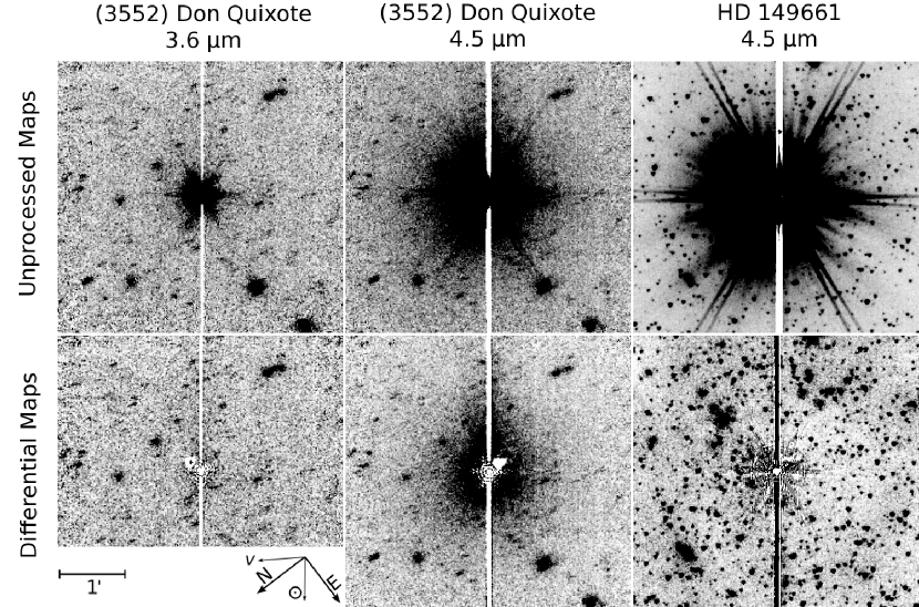
Figure 1: Inverted unprocessed (top row) and PSF–subtracted differential (bottom row) Spitzer IRAC maps of (3552) Don Quixote at 3.6 µm (left) and 4.5 µm (center), and a 4.5 µm map of the saturated calibration star HD149661 (right) for comparison. The white bars are image artifacts, caused by the well–known “column pull–down” effect (IRAC Instrument Handbook, 2012; Spitzer Observer’s Manual, 2012), observed in IRAC channel 1 and 2 mosaics. The white fringes and triangular areas in the differential mosaics are the result of a misalignment of the model and object point–spread functions (PSFs) during the subtraction, and well–understood ghost images of the overexposed target, respectively. The differential 4.5 µm map of Don Quixote clearly shows a diffuse, elongated feature centered on the saturated object that is not visible in the 3.6 µm map. The feature is extended in the anti–solar direction, as indicated in the bottom left map ($v$ indicates the velocity vector of the object). The differential mosaic of HD149661 does not show any extended emission. HD149661 is 3.8 mag brighter than Don Quixote at the time of observation; hence, any saturation effect producing the radially symmetric extended emission around Don Quixote would lead to the same effect in HD149661.

Don Quixote was observed by the Infrared Array Camera (IRAC, Fazio et al., 2004) onboard the Spitzer Space Telescope (Werner et al., 2004) on August 22, 2009, at 19:48 UT. The observations at 3.6 and 4.5 µm were taken within the ExploreNEOs program (Trilling et al., 2010), which performed thermal–infrared observations of $\sim$600 NEOs. At the time of the Spitzer observations, which took place 18 days prior to Don Quixote’s perihelion passage, the target had a heliocentric distance of 1.23 AU, a solar phase angle of 55°, and was 0.55 AU from Spitzer.

The observations (Astronomical Observation Request, AOR, 32690176) consist of 9 individual 12 sec frames in each band. The AOR used the “Moving Cluster” mode and changed the telescope pointing in such a way that the source was placed alternately on the 3.6 and 4.5 µm arrays, in order to obtain a nearly–simultaneous dataset in both bands (Trilling et al., 2010). This mode also maximizes the relative motion of the asteroid across the field in each band, making it easier to reject background emission by combination of the individual frames. Additionally, the pointing was offset relative to the predicted object position for each frame differently in order to provide dithering for each band. All frames share the same orientation in the plane of the sky: the Spitzer spacecraft and IRAC instrument designs require the Sun to be positioned below the detector array in order to provide proper shielding from sunlight. Consequentially, the Spitzer–Sun vector coincides with the pixel array columns.

Mosaics at 3.6 and 4.5 µm were constructed using the IRACproc software (Schuster et al., 2006), which aligns and combines the individual frames in each band in the rest frame of Don Quixote, based on its projected motion. Cosmic rays are filtered and rejected from the mosaic. Since Don Quixote moved only a few arc seconds during the course of the observations, the background objects in the field are not totally rejected but appear as trails in the mosaics. In the following, these maps are referred to as “unprocessed maps” in the sense of the further analysis; the maps are shown in the top row of Figure 1.

We had selected the integration time of the observations to provide adequate signal–to–noise ratio within the linear range of the detectors. However, due to a failure in the proper retrieval of the object geometry during the observation planning, the integration time was overestimated and the observations were found to be saturated in both the 3.6 and 4.5 µm bands. In order to estimate the flux of the point–like source, we apply a technique of subtracting a calibrated point–spread function (PSF) from the data. By aligning and scaling a model PSF to the observations, using a least–squares–method that minimizes the residual, the resulting scaling factor provides a measure of the object’s flux density. Only the non–saturated PSF wings and diffraction spikes are used in the scaling, the saturated regions as well as the column pull–down regions are masked off in the process (Marengo et al., 2009). Since Don Quixote was observed in the post–cryo or “Warm Spitzer” mission phase, we use a model PSF that was determined from warm mission observations of calibration stars with a range of flux densities (Hora et al., 2012; Marengo et al., 2013).

When this technique is applied to Don Quixote the derived flux density at 4.5 µm is much higher than expected, giving an unrealistically low albedo value using our default thermal modeling pipeline. A check of the 4.5 µm “differential map”, which is created by subtraction of the fitted PSF from the unprocessed map, reveals a remnant emission surrounding the core of the object (see Figure 1, bottom row). This “extended emission” is not subtracted by the fitted PSF, which means that it does not originate from a point–like but an extended source. Figure 2 compares the radial brightness profile of the unprocessed 4.5 µm image with that of the scaled PSF used in the subtraction process, revealing a discrepancy between the two caused by the extended emission. Horizontal and vertical inear brightness profiles through the nucleus also show an excess brightness towards the top of the image as shown in Figure 1, which hints towards the existence of a tail. The same PSF subtraction method applied to the 3.6 µm map does not show such remnant emission. Artifacts that are caused by the saturation of the object’s center and a misalignment of the model and image PSFs appear as bright areas in the bottom row of Figure 1.

We further investigate the emission from the point–like nucleus in Section 3.1 and the extended emission in Section 3.2, separately.

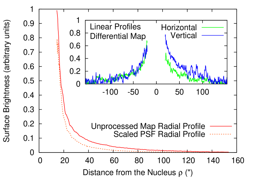
Figure 2: Radial average brightness profiles of the unprocessed 4.5 µm map (red continuous line) and the PSF scaled to fit the nucleus of Don Quixote (orange dotted line). The radial profiles were produced by averaging the pixel values in annuli with a width of 1 pixel, centered on the object center. Each point on the profile equals the median value derived from the annulus with the respective distance from the center. The space between the two lines describes the brightness of the extended emission. This plot illustrates the proper scaling of the PSF that has been used in the production of the differential image. The inlay shows the horizontal (green line) and vertical (blue line) linear brightness profiles through the center of Don Quixote, generated from the differential 4.5 µm image. Each profile represents the median of a 40–pixel wide strip centered on the respective axis (column–pull–down areas are masked). Axis definitions are the same as in the outer plot. The vicinity of the nucleus is dominated by noise caused by image artifacts and therefore not shown here. The agreement between the horizontal and vertical profiles is good below the nucleus (negative vertical distance). Above the nucleus (positive vertical distance) both profiles deviate, which is due to tail emission (see Figure 5).

2.2 Additional Observation Data

Figure 3: Don Quixote’s heliocentric distance (continuous line) and subsolar temperature (dashed line) as a function of the number of days after its perihelion passage. The dots indicate the relative position in its orbits at the time of the individual observations listed in Table 1. Observations that were performed in a different orbit cycle are marked. The subsolar temperature is based on the thermal model fit performed in Section 3.3. Spitzer IRS observations are located outside the plot and are indicated by an arrow.

We have searched the literature for previous observations of Don Quixote in various wavelength regions to compare our findings with. We did not succeed in finding reliable optical photometry that is useful for our purposes. We found useful thermal–infrared data from the literature as listed in Table 1 and discussed below. The heliocentric distance of Don Quixote at the time of the individual observations ist illustrated in Figure 3.

Table 1: Don Quixote Observations.

Observatory	Date & Time	$\lambda$	$r$	$\Delta$	$\alpha$	F	$\sigma_{F}$	Ref.
	(UT)	(µm)	(AU)	(AU)	(°)	(mJy)	(mJy)
Spitzer/IRAC	09-08-22 19:48	3.6	1.229	0.550	55.4	210	10	1
Spitzer/IRAC	09-08-22 19:48	4.5	1.229	0.550	55.4	970	50	1
Spitzer/IRS Peakup	04-03-23 04:40	16.0	6.910	6.494	7.8	6.30	0.33	1
Spitzer/IRS Spectrum	04-03-23 04:40	S	6.910	6.494	7.8	–	–	1
IRTF/SpeX	09-10-18 05:49	S	1.314	0.303	15.5	–	–	3
IRTF	83-10-13 09:21	10.1	1.574	0.664	23.1	9000	100	2
IRTF	83-10-13 10:04	10.1	1.575	0.665	23.1	7200	100	2
WISE	10-09-27 13:44	3.4	3.924	3.818	14.8	0	0.1	4
WISE	10-09-27 13:44	4.6	3.924	3.818	14.8	0	0.2	4
WISE	10-09-27 13:44	11.6	3.924	3.818	14.8	28	6	4
WISE	10-09-27 16:54	3.4	3.925	3.817	14.8	0	0.1	4
WISE	10-09-27 16:54	4.6	3.925	3.817	14.8	0	0.2	4
WISE	10-09-27 16:54	11.6	3.925	3.817	14.8	36	7	4
WISE	10-09-28 07:11	3.4	3.928	3.813	14.8	0	0.1	4
WISE	10-09-28 07:11	4.6	3.928	3.813	14.8	0.1	0.1	4
WISE	10-09-28 07:11	11.6	3.928	3.813	14.8	47	5	4
WISE	10-09-28 10:22	3.4	3.922	3.812	14.8	0	0.1	4
WISE	10-09-28 10:22	4.6	3.922	3.812	14.8	0	0.1	4
WISE	10-09-28 10:22	11.6	3.922	3.812	14.8	39	8	4

2.2.1 WISE Observations

The Minor Planet Center reports four observations of the “Wide–Field Infrared Survey Explorer” (WISE, Wright et al., 2010) of Don Quixote in September 2010 during the “3–band cryogenic” phase of the mission. The observations took place 410 days after the perihelion passage during the same orbit as the IRAC observations. The measured flux densities were accessed via the NASA/IPAC Infrared Science Archive and extracted from the “WISE 3–Band Cryo Known Solar System Object Possible Association List”. The reported magnitudes were converted into flux density units using the zeropoint magnitudes reported in Wright et al. (2010); the flux densities are listed in Table 1. See Mainzer et al. (2011), Mainzer et al. (2012), and references therein for a full discussion of asteroid observations with WISE. As it turned out, Don Quixote was too faint to be clearly detected in most of the 3.5 and 4.6 µm measurements; most of the data represent 2$\sigma$ upper limit flux densities. Low signal–to–noise observations are available at 11.6 µm.

2.2.2 IRTF Photometry

Don Quixote was observed by Veeder et al. (1989) using the NASA Infrared Telescope Facility (IRTF). They report two $N$–band magnitudes measured on October 13, 1983, which were here converted into flux density units using a calibration spectrum of Vega (Rieke et al., 2008) and are listed in Table 1. The observations of Veeder et al. (1989) took place 80 days after its perihelion, two orbits earlier than our IRAC observations.

2.2.3 IRTF SpeX Spectroscopy

Spectroscopic observations of Don Quixote have been obtained in the wavelength range 0.6–2.6 µm using the SpeX instrument (Thomas et al., 2013). SpeX (Rayner et al., 2003) is a medium resolution spectrograph and imager unit at the IRTF. The SpeX spectrum was obtained on October 18, 2009, 40 days after its perihelion passage in the same orbit of Don Quixote as the IRAC observations. Don Quixote and the solar standard star Landolt 113-276 were observed close in time. The data were reduced using SpeXtool (Cushing et al., 2004) and the telluric atmosphere correction was done using the ATRAN model atmosphere (e.g., Lord, 1992; Rivkin et al., 2004). The spectrum discussed in Section 4.3 was produced by division of the measured spectrum of Don Quixote by that of the solar analog star, resulting in a measure of the reflectance of the object’s surface. For more information on the processing of the spectrum see Thomas et al. (2013).

2.2.4 IRS Peakup Imaging and Spectroscopy

Don Quixote was also observed with the Infrared Spectrograph (IRS, Houck et al., 2004) onboard the Spitzer Space Telescope. The observations (AOR 4869888) took place on March 23, 2004, 3.2 yrs after perihelion when Don Quixote was 6.9 AU from the Sun, one orbit earlier than the Spitzer IRAC observation. The IRS observations were made using only the long wavelength, low resolution (LL) modules (LL2, 14.2 to 21.7 µm; LL2, 19.5 to 38.0 µm), including IRS Peakup observations, from which a flux density could be derived (see Table 1). All data have been processed through the standard point–source pipeline (V18.18) by the Spitzer Science Center to produce Basic Calibrated Data (BCD). During the observations, the object was nodded along the slit. We subtract the BCD frames of the two nod positions for each module to remove background flux. The data are then extracted to 1–D spectra by summing data within each constant wavelength polygon and apply the wavelength calibrations supplied by the Spitzer Science Center (SSC). We developed custom routines for IRS spectral reduction. Therefore, rather than applying the absolute flux calibration supplied by the SSC (which is valid only for their exact extraction parameters), we construct our own absolute and relative spectral calibration factors from standard stars observed by IRS throughout the mission. This method enables the flexibility to adjust the extraction width to optimize the signal–to–noise ratio. Multiple cycles and nod positions for each module are averaged, and the LL2 and LL1 spectra are scaled to each other by matching flux in the spectra range of overlap. Our reduction procedure is described in more detail by Emery et al. (2006).

3 Spitzer/IRAC Data Analysis

3.1 Emission from the Nucleus

In order to estimate the flux density of Don Quixote’s unresolved nucleus, we fit a calibrated PSF to the unsaturated regions of its image as described in Section 2.1. For the 4.5 µm map, the fit is done manually and the scaling of the PSF iterated until the residuals are minimized in the difference image. The radial profiles of the unprocessed image and the scaled PSF are shown in Figure 2. The plot shows that a significant part of the total image brightness is emission from the nucleus of Don Quixote. For an annulus with inner and outer radius of 20″ and 45″, respectively, centered on Don Quixote, more than half of the total brightness is due to emission from the nucleus. The ratio drops to 30% at radii larger than 80″. These ratios allow for a proper scaling of the PSF that is subtracted from the unprocessed map. In this work, we disregard any image data within a radius of 20″ around the nucleus of Don Quixote due to dominant image artifacts in this area, caused by the saturation and PSF subtraction. The differential maps are shown in the bottom row of Figure 1. The derived flux densities, as listed in Table 1, are those of the point–like nucleus of the object. The same method has been applied by Mommert et al. (submitted) on two other NEOs with saturated IRAC observations, not revealing similar features. For bright calibration stars, this technique achieves a typical calibration accuracy on the order of 1% (Marengo et al., 2009). In order to account for the increased calibration uncertainty of Don Quixote due to the relatively fainter core compared to the calibration standards and the difficulty caused by the extended coma emission, we add an additional 5% uncertainty in quadrature to the measured flux density uncertainties.

3.2 Emission from the Coma and the Tail

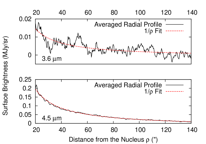
Figure 4: Radial average brightness profiles of the differential 3.6 µm (top) and 4.5 µm (bottom) maps, produced using the same method as in Figure 2. Both radial profiles were fitted over the whole range plotted here. The 3.6 µm radial profile suffers from a low signal–to–noise ratio of the emission. Nevertheless, it shows a weak trend in surface brightness versus radial distance. Both profiles have been fitted using a 1/$\rho$ relation (red dashed lines), which is the behavior expected for outgassing phenomena. The 4.5 µm radial profile agrees well with this behavior, whereas the 3.6 µm profile agrees only coarsely, due to the weak signal. Note the different scales on the vertical axes of both panels.

A detailed inspection of the IRAC maps after the PSF subtraction revealed extended emission in the form of a mostly radial symmetric coma–like structure in the 4.5 µm map (Figure 1, bottom row). In contrast, the 3.6 µm map shows no sign of a diffuse source component. The extended emission at 4.5 µm also shows a tail–like elongation towards the top of the map, pointing away from the direction towards the Sun.

In order to derive a quantitative estimate of the extended emission, we radially average the PSF–subtracted maps using a median algorithm. Areas affected by the “column–pulldown effect” (see Figure 1 and the Spitzer Observer’s Manual, 2012) are excluded from the averaging. Figure 4 shows the results of the fitting in both bands. The extended emission in the 4.5 µm map clearly follows a $1/\rho$ profile, where $\rho$ is the angular distance from the object’s center. This is the radial profile predicted for free expansion of material from a nucleus, e.g., from sublimating ices, and is characteristic of cometary comae (Jewitt & Meech, 1987). Subtracting the $1/\rho$ profile from the differential map improves the visibility of the faint cometary tail with a length of ${\sim}2$′ (see Figure 5), which points away from Sun. Note that the direction to the Sun coincides with the pixel array columns as a result of the Spitzer spacecraft design. The radial profile of the 3.6 µm map coarsely agrees with a 1/$\rho$ profile (Figure 4), despite its low signal–to–noise ratio. We measure the total flux densities of the extended emission in both bands by integrating over the fitted profiles and subtracting the background, yielding $6\pm 10$ mJy and $65\pm 10$ mJy at 3.6 and 4.5 µm, respectively. Due to the large uncertainty in the 3.6 µm flux density we adopt the derived value of 6 mJy as an upper flux density limit. The background level and its uncertainty were measured as the median and standard deviation, respectively, in four different areas of both maps that are unaffected by background sources. The measured flux densities were aperture corrected using the IRAC surface brightness correction factors (IRAC Instrument Handbook, 2012).

The derivation of the intensity of the emission from the tail suffers from the low signal and strong noise in the differential map (Figure 5), precluding a quantitative analysis of the emission from the tail.

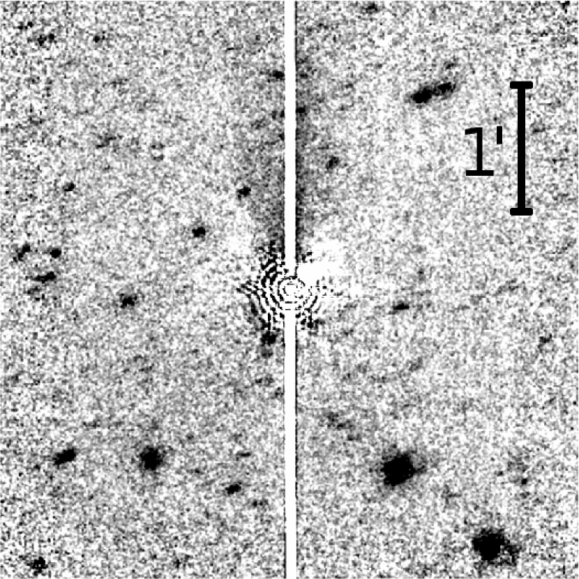
Figure 5: Don Quixote’s tail. This map shows the differential 4.5 µm map of Don Quixote from which the fitted $1/\rho$ radial profile shown in Figure 4 has been subtracted. The resulting map clearly shows the tail of Don Quixote with a length of ${\sim}2$′. The white concentric rings around the object center are image artifacts from the PSF subtraction.

3.3 Thermal Modeling of the Nucleus

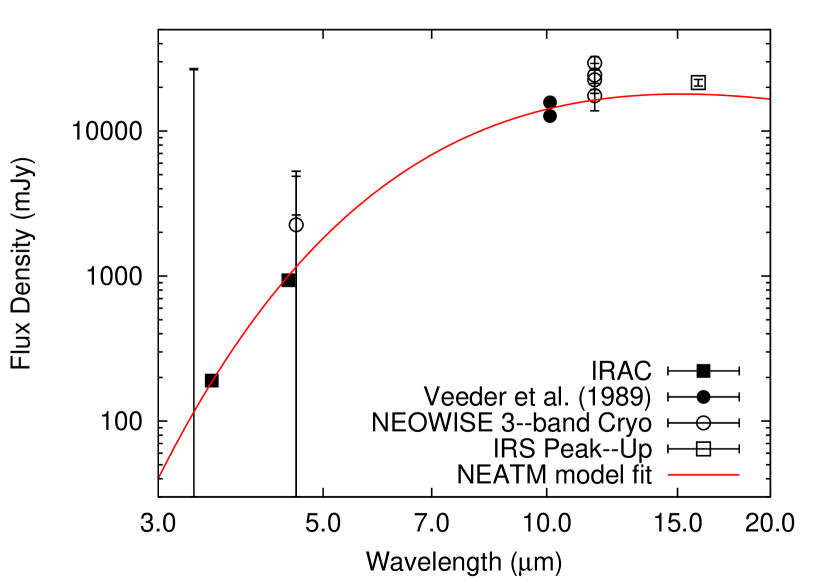
Figure 6: Thermal–model fit of Don Quixote’s nucleus. The flux densities used in the modeling and depicted in the plot are listed in Table 1. Note that all flux densities shown here are color–corrected, corrected for contributions from reflected solar light, and normalized: the individual flux densities are scaled by the ratio of the best–fit model flux densities for the respective epoch and the Spitzer IRAC epoch. Flux uncertainties are shown for each datapoint and represent 1$\sigma$ uncertainties. The line depicts the best–fit thermal model using the NEATM.

We use the Near–Earth Asteroid Thermal Model (NEATM, Harris, 1998) to derive the diameter ($d$) and the geometric $V$–band albedo ($p_{V}$) of Don Quixote’s nucleus. The NEATM combines thermal infrared and optical data to derive that set of diameter and albedo that provides the best fit to the measured spectral energy distribution. The fitting routine uses a variable beaming parameter ($\eta$, Harris, 1998) that modulates the color temperature of the model SED. The NEATM is widely used to derive the physical properties of asteroids (see, e.g., Trilling et al., 2010; Mainzer et al., 2011), as well as cometary nuclei (see, e.g., Lamy et al., 2004).

We apply the NEATM on the thermal–infrared flux densities listed in Table 1 and adopt the $H$ magnitude estimate from the Minor Planet Center ($H=13.0$ mag with an uncertainty estimate of 0.5 mag). The individual geometry for each epoch is properly taken into account in the thermal modeling. We use an iterative color correction of the IRAC, WISE and IRS Peakup data, and subtract the contributions of reflected solar light as explained in Trilling et al. (2010) and Harris et al. (2011). The resulting best–fit diameter is 18.4${}_{-0.4}^{+0.3}$ km and the albedo $p_{V}=0.03^{+0.02}_{-0.01}$, using a best–fit $\eta=0.82\pm 0.03$. Our results agree well with earlier estimates of the physical properties of Don Quixote (Veeder et al., 1989, see also Section 1). We confirm that Don Quixote is the third–largest known NEO after (1036) Ganymed (d=38.5 km, Veeder et al., 1989) and (433) Eros (d=23 km, Harris & Davies, 1999). The discovery of cometary activity in Don Quixote makes this object also one of the largest short–period comets with a measured diameter (Lamy et al., 2004). Figure 6 shows the good fit of the model spectral energy distribution to the measured thermal–infrared flux densities.

4 Discussion

4.1 Discussion of the Spitzer IRAC Data

In the following, we discuss the robustness of our observations and rule out the possibility of the extended emission to be an image artifact.

• The observed emission is not a background object. Inspection of the field of the sky in which Spitzer observed Don Quixote in the Digitized Sky Surveys (DSS, 2012), the Two Micron All Sky Survey (Skrutskie et al., 2006), as well as in WISE channels W1 (3.4 µm) and W2 (4.6 µm) of the WISE All–Sky Data Release (Cutri et al., 2012), show no extended object bright enough to be the source of the observed diffuse emission. The closest bright star, HD 22634 with $V=6.7$ mag, is separated from Don Quixote at the time of the observation by some 6.3′, outside the field of view.

• We can rule out stray–light or scattered light as the source of the emission. The stray–light and scattered–light behavior of Spitzer’s IRAC instrument is well–understood (see the IRAC Instrument Handbook, 2012; Spitzer Observer’s Manual, 2012). At the time of the IRAC observations no sufficiently bright background sources were present in the stray–light avoidance zones of either IRAC channel. In order to rule out the possibility of a contamination by stray–light or ghost images entirely, we subtract individually normalized PSFs from each of the 9 frames taken in the 4.5 µm band that were used in the generation of the unprocessed map. The position of the extended emission is centered on the object in all individual frames; the extent and intensity of the emission is equal in all frames, as well. In the case of a contamination by stray–light, the dithering would force significant variations in the intensity and position of the resulting ghost image. Hence, we can confidently rule out the possibility of the extended emission being a ghost image.

• The extended emission is not caused by latency effects. The PSF subtraction from the individual frames shows the extended emission to be centered around the object in each frame. This would not be the case if the emission were an image artifact caused by latency effects, i.e., left–over charge in the pixel wells from previous integrations, given the dithering between the individual frames.

• The extended emission is not an image artifact caused by the saturation of the object. We can rule out the possibility of the coma being an artifact caused by the saturation of the mosaics, since the detector behavior is well–characterised (IRAC Instrument Handbook, 2012; Spitzer Observer’s Manual, 2012). For comparison reasons, we have examined observations of stars with a wide range of brightness, many of which are saturated, but none of which show extended emission. As an example, we show a saturated image of calibration star HD 149961 in Figure 1, rightmost column. HD 149961 is significantly brighter ($\Delta m=3.8$ mag) than Don Quixote at the time of its observation. The image does not show any sign of radially symmetric extended emission.

• The extended emission is not an image artifact introduced by the subtraction of the PSF. We have applied the PSF subtraction technique (Marengo et al., 2009) to images of calibration stars taken during the cryogenic and “warm” mission phases of Spitzer, using the respective PSF, and found no equivalent to the extended emission observed in Don Quixote. Improper scaling of the PSF can lead to residuals in the differential image. In that case, however, residuals of the spikes would be visible, which form the brightest parts of the wings of the PSF. Improper aligning of the PSF with respect to the object leads to artifacts that do not have the radial symmetric nature of the extended emission observed in Don Quixote.

4.2 Constraining the Nature of the Emission

The nature of the extended coma–like emission is constrained by the ratio of the infrared flux densities, $F_{4.5}/F_{3.6}$, which has a value of ${\geq}9.2$, using the flux density upper limit at 3.6 µm and taking into account the 1$\sigma$ uncertainty of the 4.5 µm flux density (see Section 3.2). Based on a model for cometary dust (Kelley & Wooden, 2009; Reach et al., 2013), the expected ratio of $F_{4.5}/F_{3.6}$ for thermal emission and reflected sunlight from the dust is less than 5 for a comet at 1.23 AU from the Sun. We are confident that the source of the higher than expected 4.5 µm flux density is molecular band emission of CO (at 4.7 µm) or CO₂ (at 4.3 µm and 15.0 µm) that are stimulated by photo–dissociation and fall well within the IRAC 4.5 µm bandpass. Both molecular bands have been observed in many comets, with CO₂ typically dominating for comets in the inner Solar System (Ootsubo et al., 2012; Reach et al., 2013). Hence, we focus on a CO₂ origin of the observed emission. CO₂ molecular band emission explains the lack of extended emission in the 3.6 µm band. If the detected emission at 3.6 µm is real, it is most likely reflected solar light from dust particles that are launched from the surface by the CO₂ gas drag, according to the cometary dust model (Reach et al., 2013).

The upper limit nature of both flux density measurements of the tail (see Section 3.2) precludes the use of the $F_{4.5}/F_{3.6}$ ratio as an indicator for the nature of the emission. We suppose the nature of the tail emission to be either molecular band emission as in the coma or solar light that is reflected from dust particles. We investigate the possibility that the tail emission is solely caused by CO₂ band emission. The length of the tail shown in Figure 5 is ${\sim}2$′, which equals ${\sim}48000$ km at the distance of Don Quixote. Assuming an expansion velocity of the gas of $0.72$ km s^-1 (0.8 km s^-1 $\times\ r^{-0.5}$ with $r=1.23$ AU, Ootsubo et al., 2012), the average lifetime of the particles is required to be ${\geq}0.77$ days to be able to explain the observed tail, which is well within the lifetime for dissociation by sunlight of CO₂ (8.6 days, data from A’Hearn et al., 1995, normalized to $r=1.23$ AU assuming an inverse–square relationship between the lifetime and the heliocentric distance). Hence, we cannot exclude the possibility that the tail emission is molecular band emission.

4.2.1 Gas and Dust Production Rates

We estimate the gas and dust production rates from the measured 4.5 and 3.6 µm extended emission flux densities, respectively, assuming (1) the 3.6 µm flux density to be purely reflected solar light from dust grains, and (2) the 4.5 µm flux density to be dominated by band emission, with a contribution from thermal emission from dust. Taking into account the uncertain nature of the measured 3.6 µm flux density, we treat it as a 6 mJy upper limit.

We adopt the widely used $Af\varrho$–formalism, introduced by A’Hearn et al. (1984), to determine the properties of the dust coma, based on the assumption that the upper limit flux density at 3.6 µm is solely reflected solar light. $Af\varrho$, measured in units of cm, is the product of the dust grain bond albedo ($A$), the filling factor of the grains ($f$), and the linear radius of the field of view at the distance of the comet ($\varrho$), and is hence independent of the characteristics of the observation.

$$Af\varrho=\frac{(2\Delta r)^{2}}{\varrho}\frac{F_{c}}{F_{s}},$$ (1)

where $r$ is the heliocentric distance of the comet in AU, $\Delta$ the distance to the observer in cm, $F_{c}$ and $F_{s}$ are the measured flux density of the coma and the solar light flux density at 1 AU, respectively, in the same band. We use $F_{c}=6$ mJy with an angular radius of the aperture of 260″ and determine $F_{s}=5.7\cdot 10^{16}$ mJy by integration of the measured solar spectrum by Rieke et al. (2008) convolved with the spectral response function of the IRAC 3.6 µm band over its bandwidth. We find $Af\varrho\leq 4$ cm, which is lower than most other short–period comets (A’Hearn et al., 1995).

$Af\varrho$ can be converted into a dust production rate

$$Q_{\mathrm{dust}}=(Af\varrho)\ \frac{2}{3}\frac{\rho_{d}av_{d}}{A_{p}},$$ (2)

where $\rho_{d}$ is the dust density, $a$ the dust grain radius, $v_{d}$ the escape velocity, and $A_{p}$ the geometric albedo of the dust particles, assuming a fixed grain size (Jorda, 1995; Fornasier et al., 2013). We adopt values that are typical for short–period comets: $v_{d}=0.72$ km s^-1 (using the expansion velocity of gas: 0.8 km s^-1 $\times\ r^{-0.5}$ with $r=1.23$ AU, Ootsubo et al. (2012)), $a\sim 15$ µm (average of the range of particle sizes found for short–period comet 67P/Churyumov-Gerasimenko by Bauer et al., 2012), $\rho_{d}=1$ g cm^-3 (Bauer et al., 2012), and $A_{p}=0.15$ (Kelley & Wooden, 2009). We obtain an upper limit on the dust production rate of ${\leq}1.9$ kg s^-1. This estimate is comparable to other short–period comets (e.g., Bauer et al., 2011). Note that such a low dust production is barely detectable with optical means, as discussed in Section 4.5.

In the next step, we determine the CO₂ gas production rate from the measured 4.5 µm flux density. Firstly, we correct the measured flux density for the contribution from thermal emission from dust, based on the results derived above. We determine the contribution of thermal emission from dust as the integral over the thermal emission spectrum of dust convolved with the IRAC 4.5 µm spectral response function. The thermal emission spectrum of dust is described using a model provided by Kelley & Wooden (2009):

$$F_{\mathrm{therm}}=\frac{(1-\bar{A})}{A(\alpha)}\pi B_{\lambda}(T)\frac{(Af\varrho)}{\Delta^{2}}\varrho,$$ (3)

where $\bar{A}\sim 0.32$ is the mean bolometric Bond albedo of the dust (Gehrz & Ney, 1992), $A(\alpha)$ is the phase angle dependent Bond albedo (which is assumed to be 0.15 for $\alpha\leq 60$°, Kelley & Wooden, 2009), and $B_{\lambda}(T)$ is the Planck function with temperature $T\sim 277$ K ($=306$ K$\times 1.23^{-0.5}$, Kelley & Wooden, 2009). Given the upper limit nature of the 3.6 µm flux density measurement, we constrain that part of the emission at 4.5 µm resulting from molecular band emission to the range $51<F<65$ mJy.

We determine the CO₂ production rate based on the single–species Haser (1957) model, which describes the number density of molecules, $n$, in a distance $\varrho$ from the nucleus. The Haser model assumes the coma to be the result of a uniform, spherically symmetric outflow of molecules from a point–like nucleus at a constant speed. The emission is caused by the photo–dissociation of the CO₂ molecules. The number density (km^-3) is defined as

$$n(\varrho)=\frac{Q}{4\pi\varrho^{2}v}\ \exp(-\varrho/\gamma),$$ (4)

where $Q$ is the production rate (s^-1), $v$ the radial outflow velocity (km s^-1), and $\gamma=\tau v$, the scale length (km), which is the product of the photo–dissociation lifetime of CO₂, $\tau$ (in s^-1), and the outflow velocity. We adopt the expansion velocity of gas at the heliocentric distance of Don Quixote, $v=0.8\times 1.23^{-0.5}=0.72$ km s^-1 (Ootsubo et al., 2012) and the lifetime of CO₂, also scaled to the heliocentric distance, $\tau=5.0\cdot 10^{5}\mathrm{s}\times 1.23^{2}=7.4\cdot 10^{5}$ s. In order to derive the production rate $Q$, the column density $N(\varrho)$ in units of km^-2 has to be derived from the number density by integration along the line of sight (see, e.g., Helbert, 2003), assuming the coma to be optically thin. The column density is related to the measured flux density $F$ in units of W m^-2 µm^-1 via

$$N(\varrho)=\frac{4\pi F\cdot 10^{-9}}{Q(hc/\lambda)g\pi\varrho^{2}}\Delta^{2},$$ (5)

where $h$ is Planck’s constant, $c$ the velocity of light in vacuum, $\lambda=4.26$ µm the center wavelength of the CO₂ emission band, and $g$ the fluorescence efficiency of this band ($g=2.6\cdot 10^{-3}$ s^-1, see Footnote 6). The factor $10^{-9}$ stems from the conversion from km to µm; the aperture size for the integration of the 4.5 µm flux density is 200″. Solving this equation yields a CO₂ production rate of $Q=(1.1\pm 0.1)\cdot 10^{26}$ molecules s^-1, which is low but comparable to other short–period comets that exhibit CO₂ emission at comparable heliocentric distances (Ootsubo et al., 2012).

4.3 Constraints from Additional Data

Imaging data.

The IRTF flux density measurements from Veeder et al. (1989) have high signal–to–noise ratios (see Table 1) that might be sufficient to detect emission from a possible coma. However, the two measured flux densities deviate significantly, rising doubts about the actual accuracy of the observations and precluding further analysis.

The low signal–to–noise ratio of the WISE observations (see Table 1) precludes a search for extended emission in the image data. In the 3.4 and 4.6 µm bands of WISE, which are important for the confirmation of CO₂ band emission, Don Quixote is barely detected and only upper limit flux densities are available in all but one case.

The bandwidth of the IRS Peakup observations (13.0–18.5 µm) covers an additional CO₂ molecular emission band at 15.0 µm, which enables the search for such emission in these data. We use a method similar to the analysis of the Spitzer IRAC observations (see Section 3.2). A comparison of the radial profile of Don Quixote’s image to that of a calibration star observed near in time shows no significant differences, arguing against cometary activity. In a different approach we subtract a fitted PSF that has been modeled from a calibration star observed near in time to Don Quixote. From the residual 3$\sigma$ flux density upper limit (0.57 mJy) we derive an upper limit on the CO₂ gas production rate in the same way as in Section 4.2.1, assuming that all of the residual emission is molecular band emission from CO₂. From Equations 4 and 5 we derive $Q_{\mathrm{IRS}}\leq 13\cdot 10^{26}$ molecules s^-1 as a 3$\sigma$ upper limit, using $g=8.2\cdot 10^{-5}$ s^-1 (see Footnote 6) and $v=0.8\times 6.91^{-0.5}=0.30$ km s^-1 (Ootsubo et al., 2012). This upper limit is significantly higher than the gas production range derived in Section 4.2.1 but is still comparable to CO₂ production rates of other short–period comets (Ootsubo et al., 2012). Note that this upper limit estimation does not unambiguosly prove the existence of activity in the IRS Peakup observations.

Spectroscopic data.

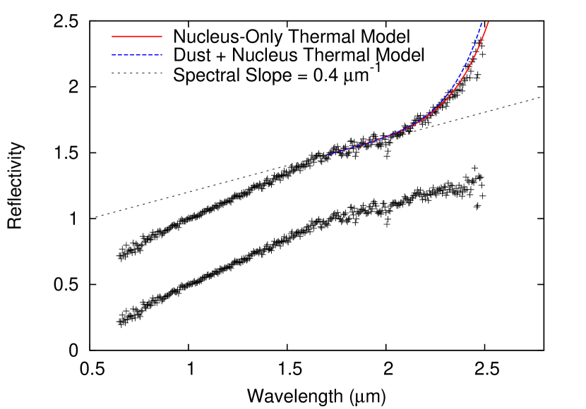
Figure 7: IRTF SpeX spectrum of Don Quixote (black crosses, top) with different emission models. The continuous red line depicts the predicted thermal emission from the nucleus, solely based on the best–fit thermal model parameters derived in Section 3.3. A possible contribution from thermal emission from dust, based on the properties of the dust coma as derived from the 3.6 µm flux density, is several orders of magnitude fainter than the emission from the nucleus and hence barely detectable. In order to derive an upper limit on the dust production rate from the spectrum, we apply an amplification factor of 100 to the predicted dust emission (dashed blue line). The lower plot shows the same spectrum, offset by 0.5 in the ordinate axis, from which the thermal tail has been subtracted, assuming the tail to be solely caused by the thermal emission from the nucleus only. Spectral data are taken from Thomas et al. (2013).

Figure 7 shows Don Quixote’s near–infrared reflectivity as a function of wavelength; the reflectivity is defined as the ratio of the measured flux density per wavelength and the spectrum of a solar analog star. The featureless spectrum has a spectral slope of ${\sim}0.7$ for $\lambda{<}1.7$ µm and ${\sim}0.4$ for $\lambda{>}1.7$ µm, which agrees with the previous classification of a D–type asteroid (Hartmann et al., 1987; Binzel et al., 2004) and other D–type asteroids (e.g., DeMeo et al., 2009; Bus et al., 2002). At the long–wavelength end of the spectrum a so–called “thermal tail” occurs where the reflectivity seems to increase dramatically as a result of contributions from thermal emission of the nucleus and/or the coma dust. We investigate the possible contribution of thermal emission from dust to the thermal tail.

The dotted line in Figure 7 presents a linear fit to the spectrum in the wavelength range 1.7–2.1 µm that is unaffected by the thermal tail. We compute the thermal emission spectrum of the nucleus and the dust coma for this wavelength range using the thermal model of the nucleus (see Section 3.3) and the model for thermal emission from dust (Equation 3), respectively. The dust emission model is based on an aperture size that equals the length of the spectrograph slit (60″). The thermal emission from dust is several orders of magnitude fainter than the emission from the nucleus and barely affects the shape of the spectrum. The emission from the nucleus is shown as a continuous red line in Figure 7. The line fits the data points well without using any fitting to the data. The dashed blue line shows the thermal model of the nucleus combined with a model for thermal emission from dust that assumes a 100 times higher dust production rate. The combined emission model still agrees with the measured spectrum and translates into an upper limit of the dust production rate of 190 kg s^-1. The upper limit is significantly higher than the value derived from IRAC observations, but does not prove the presence of activity in the spectral data.

We take a different approach in the analysis of the IRS spectral data, since the simultaneously acquired IRS Peakup data revealed no clear evidence for cometary activity. We apply a NEATM fit to the calibrated spectrum, yielding a diameter of 18.8$\pm$1.5 km and an albedo of 0.03$\pm$0.01 (assuming $H=13.0$), with a best–fit $\eta=0.7\pm 0.1$. The physical properties derived from the spectrum agree well with the results obtained from the photometric data in Section 3.3.

Despite the low signal–to–noise ratio of the IRS spectrum of Don Quixote (Figure 8), clear emissivity peaks are apparent near 20 and 34 µm. Roughly similar emissivity peaks occur in spectra of comets and primitive asteroids, indicating the presence of fine–grain silicates. The Don Quixote spectrum lacks a peak at 24 µm that is present in many comets and in D–type Trojan asteroids. This feature is due to olivine, and we interpret its absence, on Don Quixote, along with the overall shape and position of the ${\sim}$20 µm peak, to indicate a more pyroxene–rich surface than those other objects.

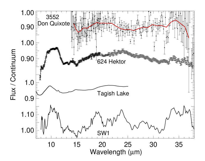
Figure 8: Comparison of the Don Quixote IRS spectrum (top) with that of D–type asteroid (624) Hektor (Emery et al., 2006), a sample of the Tagish Lake meteorite (Hiroi et al., 2001), and short–period comet 29/P Schwassmann–Wachmann 1 (Stansberry et al., 2004). The continuous red line indicates a running average over the Don Quixote spectrum and exhibits increased emissivity around 20 and 34 µm. The spectrum of Don Quixote shows significant differences to those of the other objects presented here.

4.4 Cause and Longevity of the Activity

The evidence for CO₂ band emission implies the existence of CO₂ ice on Don Quixote. The ice is presumably buried under a thick layer of insulating material (Rickman et al., 1990) to explain its existence in near–Earth space. Two scenarios can explain the observed activity: (1) subsurface CO₂ sublimates due to seasonal heating, causing persistent activity, or (2) the observed activity is temporary, e.g., triggered by a recent impact that exposed icy sub–surface material, leading to a brief activity outbreak. The proximity of Don Quixote to the Sun ($r=1.23$ AU) during the IRAC observations is equally consistent with both of the aforementioned scenarios.

Because cometary activity was only unambiguously detected in the IRAC observations, no direct conclusions regarding the cause and longevity of the discovered activity can be drawn. However, a comparison with previous work is informative. Kelley et al. (2013) found in their “Survey of the Ensemble Properties of Cometary Nuclei” (SEPPCON) that all short–period comets in their sample with $q<1.8$ AU (30 objects) are inactive, presumably because they have already lost all of their volatiles. The SEPPCON sample targets are known comets that have shown persistent activity at least in the past. Don Quixote, showing activity with a perihelion distance of only $q=1.21$ AU, presents an exception to the findings of Kelley et al. (2013). Hence, we speculate that the observed behavior in Don Quixote is most consistent with a temporary outbreak of activity.

Further observations are necessary to unambiguously constrain the cause and longevity of the activity. Additional observations during the next perihelion passage in May 2018 will help to resolve the nature of Don Quixote’s activity.

4.5 Implications of this Discovery

Because they are spectrally featureless and have no clear meteorite analog, compositions of D–type asteroids like Don Quixote (Hartmann et al., 1987; Binzel et al., 2004) are poorly constrained. (Vernazza et al., 2013) showed that the one meteorite fall that was originally associated with a D–type spectrum, Tagish Lake (Brown et al., 2000; Hiroi et al., 2001), is not representative for D–type asteroids. Nevertheless, the low albedo of Don Quixote suggests a carbonaceous surface material that is generally rich in water and carbon and at least similar to the Tagish Lake meteorite. Hence, we use the composition of the Tagish Lake meteorite as an analog for carbonaceous material. The meteorite has a total water fraction of 3.9 weight percent (wt%, Baker et al., 2002) and a total organic carbon fraction of 2.6 wt% (Grady et al., 2002). Assuming a spherical shape for Don Quixote and a homogeneous composition identical to that of the Tagish Lake meteorite with a density of 1.5 g cm^-3 (Brown et al., 2000), we estimate the total mass of Don Quixote as ${\sim}5\cdot 10^{15}$ kg. Based on this mass, the total water content of Don Quixote would be ${\sim}2\cdot 10^{14}$ kg, which equals the amount of water in the upper–most 1.5 mm of Earth’s oceans. The total organic carbon content of Don Quixote is ${\sim}1.3\cdot 10^{14}$ kg. These estimates show that the impact of such an object could add significant amounts of water and organic material to Earth’s inventory.

Don Quixote has long since been suspected to be of cometary origin as a result of its comet–like orbit (e.g., Hahn & Rickman, 1985; Weissman et al., 1989) and albedo (Veeder et al., 1989). Furthermore, dynamical models clearly suggest a cometary origin (Bottke et al., 2002). The discovery of activity in this object would not be surprising if the object had not been lacking any sign of activity in previous observations. We suppose that Don Quixote’s activity evaded discovery due to either its intermittent nature or, if persistent, the fact that it is triggered by the sublimation of CO₂ ice, the band emission of which is not observable in the optical. This assertion is supported by the low amount of reflected solar light from dust ($Af\varrho\leq 4$ cm, which translates into a $V$–band surface brightness of $\sim$26 mag/square arcsecond), which we derived from the IRAC 3.6 µm flux density. For comparison, the data compiled in A’Hearn et al. (1995) show that most known comets with heliocentric distances comparable to that of Don Quixote have $Af\varrho\sim 100$ cm. If we assume this value to be a rough threshold that triggers the detection of cometary activity by optical means, the observed dust production rate, which is linearly related to $Af\varrho$ (see Equation 2), would have to be at least one order of magnitude higher.

The existence of CO₂ puts constraints on Don Quixote’s origin and evolution: its interior must have formed at very low temperatures (${\leq}60$ K) to condense CO₂ and must have remained cold since (Yamamoto, 1985). The subsurface layers of Don Quixote that contain CO₂–ice are required to have temperatures of 60 K and below in order to retain the ice. This implies that the diurnal and seasonal heat waves do not affect the ice layers and are absorbed in the near–surface insolation layer.

CO₂ band emission has been detected in a number of short–period comets (Ootsubo et al., 2012). Our discovery implies that other NEOs of cometary origin can retain deposits of CO₂ and other volatiles in the same way as Don Quixote. Such objects might show temporary activity and evade discovery by optical means at the same time. Hence, we suggest expanded monitoring of likely dormant and/or extinct comets to infrared wavelengths close in time to their perihelion passage in order to detect CO₂ band emission at 4.3 µm.

4.6 Summary

• We find evidence for cometary activity in NEO (3552) Don Quixote, the third–largest object in near–Earth space, based on Spitzer IRAC observations. Extended emission has been detected in the 4.5 µm band observations, but only marginally so at 3.6 µm. We interpret the lack of a clear detection of a coma at 3.6 µm as indicating that activity is caused by band emission from CO₂. The 4.5 µm extended emission shows an anti–sunward directed tail with a length of ${\sim}2$′.

• From the 3.6 µm band flux–density measurement we determine an upper limit on the dust production rate of ${\leq}1.9$ kg s^-1. Using this estimate and the 4.5 µm flux density measurement, we constrain a CO₂ production rate at the time of the Spitzer observations of $(1.1\pm 0.1)\cdot 10^{26}$ molecules s^-1.

• The IRAC observations combined with the additional observations from the literature allow for a robust thermal model fit of Don Quixote’s nucleus, yielding a diameter and albedo of 18.4${}_{-0.4}^{+0.3}$ km and $0.03^{+0.02}_{-0.01}$, respectively. Our results confirm that Don Quixote is the third–largest known NEO and indicate that it is one of the largest known short–period comets.

• Spectroscopic observations agree with a D–type classification of Don Quixote and suggest the presence of fine–grained silicates, perhaps pyroxene rich, on its surface.

• We suspect that Don Quixote’s activity has evaded discovery to date due to either its possibly intermittent nature or, if persistent, the fact that it is triggered by the sublimation of CO₂ ice, the band emission of which is not observable in the optical.

References

- A’Hearn et al. (1984) A’Hearn, M. F., Schleicher, D. G., Millis, R. L. et al., 1984, AJ, 89, 579
- A’Hearn et al. (1995) A’Hearn, M. F., Millis, R. L., Schleicher, D. G. et al., 1995, Icarus, 118, 223
- Baker et al. (2002) Baker, L., Franchi, I. A., Wright, I. P., Pillinger, C. T., 2002, M&PS, 37, 977
- Bauer et al. (2011) Bauer, J. M., Walker, R. G., Mainer, A. K. et al., 2011, ApJ, 738, 171
- Bauer et al. (2012) Bauer, J. M., Kramer, E., Mainzer, A. K. et al, 2012, ApJ, 758, 18
- Binzel et al. (2004) Binzel, R. P., Rivkin, A. D., Stuart, J. S. et al., 2004, Icarus, 170, 259
- Bottke et al. (2002) Bottke, W. F., Morbidelli, A., Jedicke, R. et al., 2002, Icarus, 156, 399
- Bowell et al. (1992) Bowell, E., Buie, M. W., Picken, H., 1992, IAU Circ., 5586, 1
- Brown et al. (2000) Brown, P. G., Hildebrand, A. R., Zolensky, M. E. et al., 2000, Science, 290, 320
- Bus et al. (2002) Bus, S. J., Binzel, R. P., 2002, Icarus, 158, 106
- Cushing et al. (2004) Cushing, M. C., Vacca, W. D., Rayner, J. T., 2004, PASP, 116, 362
- Cutri et al. (2012) Cutri, R. M., Wright, E. L., Conrow, T. et al., 2012, Explanatory Supplement to the WISE All-Sky Data Release Products, http://wise2.ipac.caltech.edu/docs/release/allsky/expsup/index.html
- DeMeo et al. (2009) DeMeo, F. E., Binzel, R. P., Slivan, S. M., Bus, S. J., 2009, Icarus, 202, 16
- Emery et al. (2006) Emery, J. P., Cruikshank, D. P., van Cleve, J., 2006, Icarus, 182, 496
- Fazio et al. (2004) Fazio, G. G., Hora, J. L., Allen, L. E. et al., 2004, ApJS, 154, 10
- Fernández et al. (1997) Fernández, Y. R., Mc Fadden, L. A., Lisse, C. M. et al., 1997, Icarus, 128, 114
- Warner & Fitzsimmons (2005) Warner, B. D., Fitzsimmons, A., IAU Circ., 8578, 1
- Fornasier et al. (2013) Fornasier, S., Lellouch, E., Müller, T. G. et al., 2013, A&A, 555, A15
- Gehrz & Ney (1992) Gehrz, R. D., Ney, E. P., 1992, Icarus, 100, 162
- Grady et al. (2002) Grady, M. M., Verchovsky, A. B., Franchi, I. A., Wright, I. P., Pillinger, C. T., 2002, M&PS, 37, 713
- Hahn & Rickman (1985) Hahn, G., Rickman, H., 1985, Icarus, 61, 417
- Harris (1998) Harris, A. W., 1998, Icarus, 131, 291
- Harris & Davies (1999) Harris, A. W., Davies, J. K., 1999, Icarus, 142, 464
- Harris et al. (2011) Harris, A. W., Mommert, M., Hora, J. L. et al., 2011, AJ, 141, 75
- Hartmann et al. (1987) Hartmann, W. K., Tholen, D. J., Cruikshank, D. P., 1987, Icarus, 69, 33
- Haser (1957) Haser, L., 1957, Bulletin de la Societe Royale des Sciences de Liege, 43, 740
- Helbert (2003) Helbert, J., 2003, PhD thesis, Freie Universität Berlin
- Hiroi et al. (2001) Hiroi, T., Zolensky, M. E., Pieters, C.M., 2001, Science, 293, 2234
- Hora et al. (2012) Hora, J. L., Marengo, M., Park, R. et al., 2012, Proc. SPIE, 8442, 39
- Houck et al. (2004) Houck, J. R., Roellig, T. L., van Cleve, J. et al., 2004, ApJS, 154, 18
- Jewitt & Meech (1987) Jewitt, D. C., Meech, K. J., 1987, ApJ, 317, 992
- Jorda (1995) Jorda, L., 1995, PhD thesis, University of Paris
- Kelley & Wooden (2009) Kelley, M. S., Wooden, D. H., 2009, Planetary and Space Science, 57, 1133
- Kelley et al. (2013) Kelley, M. S., Fernández, Y. R., Licandro, J. et al., 2013, Icarus, 225, 475
- Lamy et al. (2004) Lamy, P. L., Toth, I., Fernandez, Y. R., Weaver, H. A., 2004, Comets II, University of Arizona Press, Tucson
- Levison & Duncan (1997) Levison, H. F., Duncan, M. J., 1997, Icarus, 127, 13
- Lord (1992) Lord, S. D., 1992, NASA Technical Memorandum 103957
- Mainzer et al. (2011) Mainzer, A., Grav, T., Bauer, J. et al., 2011, ApJ, 743, 17
- Mainzer et al. (2012) Mainzer, A., Grav, T., Masiero, J. et al., 2012, ApJL, 760, L12
- Marengo et al. (2009) Marengo, M., Stapelfeldt, K., Werner, M. W. et al., 2009, ApJ, 700, 1647
- Marengo et al. (2013) Marengo, M. et al., 2013, in preparation
- Mommert et al. (submitted) Mommert, M., Harris, A. W., Mueller, M. et al., 2013, AJ, submitted
- Morbidelli & Gladman (1998) Morbidelli, A., Gladman, B., 1998, M&PS, 33, 999
- Ootsubo et al. (2012) Ootsubo, T., Kawakita, H., Hamada, S. et al., 2012, ApJ, 752, 15
- Rayner et al. (2003) Rayner, J. T., Toomey, D. W., Onaka, P. M. et al., 2003, PASP, 115, 362
- Reach et al. (2013) Reach, W. T., Kelley, M., and Vaubaillon, J., 2013, Icarus, 226, 777
- Rickman et al. (1990) Rickman, H., Fernandez, J. A., Gustafson, B. A. S., 1990, A&A, 237, 524
- Rieke et al. (2008) Rieke, G. H., Blaylock, M., Decin, L. et al., 2008, AJ, 135, 2245
- Rivkin et al. (2004) Rivkin, A. S., Binzel, R. P., Sunshine, J. et al., 2004, Icarus, 172, 408
- Schuster et al. (2006) Schuster, M. T., Marengo, M., Patten, B. M., 2006, Proc. SPIE, 6270, 20
- Skrutskie et al. (2006) Skrutskie, M.F., Cutri, R. M., Stiening, R. et al., 2006, AJ, 131, 1163
- Stansberry et al. (2004) Stansberry, J. A., Van Cleve, J., Reach, W. T. et al., 2004, ApJS, 154, 463
- DSS (2012) Space Telescope Science Institute, The Digitized Sky Survey, 2012, http://archive.stsci.edu/cgi-bin/dss_form
- Spitzer Observer’s Manual (2012) Spitzer Science Center, 2012, Spitzer Space Telescope Observer’s Manual, Version 11.1, http://ssc.spitzer.caltech.edu/warmmission/propkit/som/
- IRAC Instrument Handbook (2012) Spitzer Science Center, 2012, IRAC Instrument Handbook, Version 2.0.2, http://irsa.ipac.caltech.edu/data/SPITZER/docs/irac/iracinstrumenthandbook/
- Thomas et al. (2013) Thomas, C. A., Emery, J. P., Trilling, D. E., Delbo’, M., Hora, J. L. et al. 2004, Icarus, 228, 217
- Trilling et al. (2010) Trilling, D. E., Mueller, M., Hora, J. L. et al., 2010, AJ, 140, 770
- Veeder et al. (1989) Veeder, G.J., Hanner, M. S., Matson, D. L. et al., 1989, AJ, 97, 1211
- Vernazza et al. (2013) Vernazza, P., Fulvio, D., Brunetto, R. et al., 2013, Icarus, 225, 517
- Weissman et al. (1989) Weissman, P. R., A’Hearn, M. F., Mc Fadden, L. A. et al., 1989, Asteroids II, Univ. Arizona Press, Tucson
- Weissman et al. (2002) Weissman, P. R., Bottke, W. F., and Levison, H. F., 2002, Asteroids III Univ. Arizona Press, Tucson
- Werner et al. (2004) Werner, M. W., Roellig, T. L., Low, F. J. et al., 2004, ApJS, 154, 1
- Wetherill & Williams (1979) Wetherill, G. W., Williams, J. G., 1979, Origin and distribution of the elements, Volume 34, Pergamon Press Ltd., London
- Wright et al. (2010) Wright, E. L., Eisenhardt, P. R. M., Mainzer, A. K. et al., 2010, AJ, 140, 1868
- Yamamoto (1985) Yamamoto, T., 1985, A&A, 142, 31