Positivity constraints on the low-energy constants
of the chiral pion-nucleon Lagrangian

Abstract

Positivity constraints on the pion-nucleon scattering amplitude are derived in this article with the help of general S-matrix arguments, such as analyticity, crossing symmetry and unitarity, in the upper part of Mandelstam triangle, ${\cal R}$. Scanning inside the region ${\cal R}$, the most stringent bounds on the chiral low energy constants of the pion-nucleon Lagrangian are determined. When just considering the central values of the fit results from covariant baryon chiral perturbation theory using extended-on-mass-shell scheme, it is found that these bounds are well respected numerically both at the $O(p^{3})$ and $O(p^{4})$ level. Nevertheless, when taking the errors into account, only the $O(p^{4})$ bounds are obeyed in the full error interval, while the bounds on $O(p^{3})$ fits are slightly violated. If one disregards loop contributions, the bounds always fail in certain regions of ${\cal R}$. Thus, at a given chiral order these terms are not numerically negligible and one needs to consider all possible contributions, i.e., both tree-level and loop diagrams. We have provided the constraints for special points in $\mathcal{R}$ where the bounds are nearly optimal in terms of just a few chiral couplings, which can be easily implemented and employed to constrain future analyses. Some issues about calculations with an explicit $\Delta$ resonance are also discussed.

I Introduction

Chiral perturbation theory ($\chi$PT ) ChPT plays an important role in studying low energy hadron physics, such as the pion-nucleon interaction. Many efforts have been made to study pion-nucleon physics within baryon chiral perturbation theory (B$\chi$PT) gasser using different approaches, e.g., heavy baryon (HB) $\chi$PT HB , infrared regularization (IR) IR , extended on mass shell (EOMS) EOMS , etc. The scattering amplitudes are then expressed in terms of the low energy constants (LECs). As it is well known, when stepping up to higher and higher orders, there always appears a rapidly growing number of LECs, which are free parameters, not fixed by chiral symmetry. Nevertheless, general S-matrix arguments such as analyticity, crossing and unitarity can be used to constrain the pion-nucleon interaction and its chiral effective theory description. It is therefore possible to obtain certain model-independent constraints on the LECs.

Along this line, many works have been devoted to the study of positivity constraints on $\pi\pi$ scattering amplitudes (e.g., see Refs. Ananthanarayan ; Dita ; Manohar ; Mateu ; Guo ). The pion-nucleon scattering was also studied in Ref. Luo , in terms of the pion energy $E_{\pi}$ in the center-of-mass rest-frame and positivity constraints were extracted for the second derivative of the $\pi^{\pm}p\to\pi^{\pm}p$ scattering amplitude with respect to $E_{\pi}$. However, only the $\pi^{+}p$ forward scattering ($t=0$) was analyzed in detail and no extra information was extracted from the $\pi^{-}p$ channel. Likewise, the positivity of its second derivative was only analyzed at two particular points, $E_{\pi}=\pm M_{\pi}/\sqrt{2}$ Luo . The central values from HB-$\chi$PT HBp3 were employed to check the obtained bounds.

In this paper, the analysis is extended beyond the forward case $t=0$ to the full upper part of the Mandelstam triangle ${\cal R}$ (with $t>0$). In Sec. II we introduce the general properties of pion-nucleon scattering. A particular combination $D_{\alpha}$ of the pion-nucleon scattering functions $A(s,t)$ and $B(s,t)$ is written down in terms of a positive definite spectral function in Sec. III. It is then used to extract the positivity constraints for both $\pi^{\pm}p\to\pi^{\pm}p$ scatterings in Sec. IV. Hence, compared to Ref. Luo , extra information coming from the $B(s,t)$ function and the $\pi^{-}p\to\pi^{-}p$ scattering is taken into consideration in the present work. Rather than taking two particular points to get two bounds, we scan the full region ${\cal R}$, extracting the most stringent bounds on the LECs. These are then tested in Sec. V by means of the recent results from relativistic B$\chi$PT using EOMS scheme oller ; yao . This scheme is more convenient for our analysis than the HB$\chi$PT ones, as EOMS-B$\chi$PT possesses the correct analytic behaviour in the Mandelstam triangle. The uncertainties due to the LEC errors and the impact of the $\Delta$ resonance are also analyzed in Sec. V. The conclusions are summarized in Sec. VI and some technical details about the positivity of the right-hand cut spectral function are relegated to the Appendix.

II Aspects of elastic pion-nucleon scattering

The effective Lagrangian describing the low-energy pion-nucleon scattering at $O(p^{4})$ level takes the following form:

$${\cal L}_{\pi N} = \bar{\Psi}\left\{i\,\not{D}-m+\frac{g}{2}\,\not{u}\gamma_{5}+\sum_{i=1}^{7}c_{i}\,{\cal O}^{(2)}_{i}+\sum_{j=1}^{23}d_{j}\,{\cal O}^{(3)}_{j}+\sum_{k=1}^{118}e_{k}\,{\cal O}^{(4)}_{k}\right\}\Psi+\cdots$$ (1)

where ${\cal O}_{i}^{(m)}$s ($m=2,3,4$) are the operators of $O(p^{m})$. Their explicit expressions can be found in Ref. eff and the references therein. Here $m$ and $g$ denote the nucleon mass and the axial charge in the chiral limit. The coefficients $c_{i},d_{j},e_{k}$ are LECs, given in units of GeV^-1, GeV^-2 and GeV^-3, respectively.

In the isospin limit, the scattering amplitude for the process of $\pi^{a}(q)+N(p)\to\pi^{a^{\prime}}(q^{\prime})+N(p^{\prime})$ with isospin indices $a$ and $a^{\prime}$ is described by $A^{\pm}(s,t)$, $B^{\pm}(s,t)$ and $D^{\pm}(s,t)$ according to gasser ; pinbecher

$$T_{\pi N}^{a^{\prime}a}(s,t) = \chi_{N^{\prime}}^{\dagger}\,\bigg{\{}\,\frac{1}{2}\{\tau_{a^{\prime}},\tau_{a}\}T^{+}(s,t)+\frac{1}{2}[\tau_{a^{\prime}},\tau_{a}]T^{-}(s,t)\,\bigg{\}}\,\chi_{N}\ ,$$ (2)

$$T^{\pm}(s,t) = \bar{u}(p^{\prime})\left[A^{\pm}(s,t)+\frac{\not{q}^{\prime}+\not{q}}{2}B^{\pm}(s,t)\right]u(p)=\bar{u}(p^{\prime})\left[D^{\pm}(s,t)+\frac{[\not{q}^{\prime},\not{q}]}{4m_{N}}B^{\pm}(s,t)\right]u(p)\ ,$$ (3)

$$D^{\pm}(s,t) = A^{\pm}(s,t)+\nu B^{\pm}(s,t)\ ,$$ (4)

here $\tau_{a^{\prime}}$, $\tau_{a}$ are Pauli matrices, $\nu=(s-u)/{4m_{N}}$ and $\chi_{N}$ ($\chi_{N^{\prime}}$) is the isospinor for the incoming (outgoing) nucleon. The Mandelstam variables s, t and u fulfill $s+t+u=2m_{N}^{2}+2M_{\pi}^{2}$ with $m_{N}$ and $M_{\pi}$, being the physical nucleon and pion masses, respectively. The functions $X^{\pm}$ with $X=\{A,B,D\}$ are the so-called isospin-even (for ‘+’) and -odd (for ‘-’) amplitudes, and they are related to the isospin amplitudes with definite isospin $I$ ($1/2$ or $3/2$) via

$$X^{1/2}=X^{+}+2X^{-}\ ,\qquad X^{3/2}=X^{+}-X^{-}\ .$$ (5)

It is also convenient for later use to write down the relations among the $\pi^{\pm}p\to\pi^{\pm}p$ scattering amplitudes , isospin even/odd amplitudes and isospin amplitudes:

$$X^{\pi^{+}p}\,=\,X^{3/2}\,=\,X^{+}\,-\,X^{-}\ ,\qquad\qquad X^{\pi^{-}p}\,=\,\frac{2}{3}X^{1/2}\,+\,\frac{1}{3}X^{3/2}\,=\,X^{+}\,+\,X^{-}\ .$$ (6)

The physical region for the pion-nucleon reaction corresponds to the kinematical region where the Kibble function Kibble $\Phi=t\left[su-(m_{N}^{2}-M_{\pi}^{2})^{2}\right]$ is non-negative. In Fig. 1, the physical regions are depicted by light gray. The triangle in the center is given by $s,\,u\leq(m_{N}+M_{\pi})^{2}$ and $t<4M_{\pi}^{2}$. It is the so-called Mandelstam triangle. The upper part of the Mandelstam triangle bounded by $t\geq 0$ corresponds to the region ${\cal R}$ (marked in red in Fig. 1) where the positivity conditions are considered. In terms of the $(\nu,t)$ variables the Mandelstam diagram is given by $t\leq 4M_{\pi}^{2}$ and $|\nu|\leq\nu_{th}(t)=M_{\pi}+t/(4m_{N})$. In order to obtain the region $\mathcal{R}$ one should add the restriction $t\geq 0$.

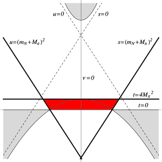
Figure 1: Mandelstam plane $(\nu,t)$. The Mandelstam triangle is the region contoured by the $s=(m_{N}+M_{\pi})^{2}$, $u=(m_{N}+M_{\pi})^{2}$ and $t=4M_{\pi}^{2}$ lines. Our region of study $\mathcal{R}$ is the trapezium formed by the three previous lines and $t=0$, which is marked in red.

III Partial wave decomposition and positive definite spectral function

It is well known that the full isospin amplitude can be written in terms of the partial-wave (PW) amplitudes as roy-steiner

$$\vec{{\cal A}}^{I}(s,t)\bigg{|}_{t=t(s,z_{s})}=\sum_{\ell=0}^{\infty}S^{\ell}(s,z_{s})\vec{{\cal F}}_{\ell}^{I}(s)\ ,$$ (7)

with

$$\vec{{\cal A}}^{I}\equiv\left(\begin{array}[]{c}A^{I}\\ B^{I}\\ \end{array}\right)\ ,\quad\vec{F}^{I}_{\ell}\equiv\left(\begin{array}[]{c}f_{\ell+}^{I}\\ f_{(\ell+1)-}^{I}\\ \end{array}\right)\ ,$$ (12)

and

$$S^{\ell}(s,z_{s})=4\pi\left(\begin{array}[]{cc}\left[\frac{W+m_{N}}{E+m_{N}}P_{\ell+1}^{\prime}(z_{s})+\frac{W-m_{N}}{E-m_{N}}P_{\ell}^{\prime}(z_{s})\right]&-\left[\frac{W+m_{N}}{E+m_{N}}P_{\ell}^{\prime}(z_{s})+\frac{W-m_{N}}{E-m_{N}}P_{\ell+1}^{\prime}(z_{s})\right]\\ \left[\frac{1}{E+m_{N}}P_{\ell+1}^{\prime}(z_{s})-\frac{1}{E-m_{N}}P_{\ell}^{\prime}(z_{s})\right]&-\left[\frac{1}{E+m_{N}}P_{\ell}^{\prime}(z_{s})-\frac{1}{E-m_{N}}P_{\ell+1}^{\prime}(z_{s})\right]\\ \end{array}\right)\ ,\quad W=\sqrt{s}.$$ (15)

Here $P_{\ell}(z_{s})$ are the conventional Legendre polynomials and $z_{s}=1+\frac{2s\,t}{\lambda(s,m_{N}^{2},M_{\pi}^{2})}$ with $\lambda(s,m_{N}^{2},M_{\pi}^{2})=[s-(m_{N}+M_{\pi})^{2}][s-(m_{N}-M_{\pi})^{2}]$, is the K$\ddot{a}$ll$\acute{e}$n function. These set of kernel matrices $S^{\ell}(s,z_{s})$ are always analytical functions, real for real values of the Mandelstam variables $(s,t,u)$. Thus, in the case $s\geq s_{th}$ the whole analytic discontinuity is due to the partial waves $f^{I}_{k}(s)$:

$${\rm Im}\vec{\cal A}^{I}(s+i\epsilon,t)=\sum_{\ell=0}^{\infty}S^{\ell}(s,z_{s}(s,t))\ {\rm Im}\vec{\cal F}^{I}(s+i\epsilon)\ .$$ (16)

Since a fixed–$t$ dispersion relation for the analysis of the subthreshold amplitude will be used in Sec. IV, our interest is focused on obtaining a positive definite spectral function in the physical region $s\geq s_{th}$. On the right-hand side of Eq. (16), the imaginary part of each PW is positive due to unitarity, i.e., ${\rm Im}f_{k}^{I}(s)\geq 0$ for $s\geq s_{\rm th}$, but the kernel matrices always contain negative elements. Therefore, it is proper to construct a combination of $A^{I}$ and $B^{I}$ in the form

$$D_{\alpha}^{I}(s,t)\equiv\alpha A^{I}(s,t)+\nu B^{I}(s,t)=\alpha D^{I}(s,t)+(1-\alpha)\nu B^{I}(s,t)$$ (17)

such that its imaginary part satisfies

$${\rm Im}D_{\alpha}^{I}(s,t)\geq 0\ .$$ (18)

In order to guarantee Eq. (18), it is proven in great detail in App. A that the validity region for the combination factor $\alpha$ should be $\alpha_{\rm min}(t)\leq\alpha\leq\alpha_{\rm max}(t)$ with

$$\alpha_{\rm min}(t)\,=\,\frac{\displaystyle\left(1+\frac{t}{4m_{N}M_{\pi}}\right)\,\left(1-\frac{t}{4m_{N}^{2}}\right)}{\displaystyle\left(1+\frac{t}{2m_{N}M_{\pi}}+\frac{t}{4m_{N}^{2}}\right)}\,=\,1\,-\,\frac{\displaystyle t}{\displaystyle 4m_{N}M_{\pi}}\,+\,{\cal O}\bigg{(}\frac{\displaystyle p^{2}}{\displaystyle m_{N}^{2}}\bigg{)}\,,\qquad\qquad\alpha_{\rm max}(t)\,=\,1+\frac{t}{4m_{N}M_{\pi}}\,,$$ (19)

where $M_{\pi}={\cal O}(p)$ and $t={\cal O}(p^{2})$ oller ; yao .

It is worth noting that here the Mandelstam variable $t$ must be greater than zero, i.e., $t\geq 0$, due to the application of Eq. (77) and the fact of $P_{k}^{\prime}(z_{s})\geq 0$ for $z_{s}\geq 1$ in App. A. This is the reason why our analysis of the positivity constraints is restricted to the upper part of the Mandelstam triangle ${\cal R}$ (see Fig 1).

So far, the $s$-channel positive definite spectral function above threshold is clear. The corresponding $u$-channel one is easily obtainable by crossing symmetry:

$$D_{\alpha}^{I}(u,t)=C_{LR}^{II^{\prime}}D_{\alpha}^{I^{\prime}}(s,t)\ ,\quad\text{(or, equivalently, $D_{\alpha}^{I}(-\nu,t)=C_{LR}^{II^{\prime}}D_{\alpha}^{I^{\prime}}(\nu,t)$)}$$ (20)

with the crossing matrix being

$$C_{LR}=\frac{1}{3}\left(\begin{array}[]{cc}-1&4\\ 2&1\\ \end{array}\right)\ ,\quad C_{LR}^{II^{\prime}}C_{LR}^{I^{\prime}J}=\delta_{IJ}\ .$$ (23)

where the first (second) row and column of $C_{LR}$ correspond to isospin $\frac{1}{2}$ (isospin $\frac{3}{2}$). $C_{LR}$ can be also sometimes denoted in the bibliography as $C_{u}$.

IV Theoretical constraints indicated by the dispersion relation

For $0\leq t\leq 4M_{\pi}^{2}$ it is possible to write down a fixed–$t$ dispersion relation for the $X(\nu,t)$ in terms of the $\nu$ variable (or $s$, if desired). If $\nu D^{I}_{\alpha}(\nu,t)$ vanished for $|\nu|\to\infty$, the amplitude $D_{\alpha}^{I}(\nu,t)$ could be represented then by the unsubtracted dispersive integral,

$$D_{\alpha}^{I}(\nu,t) = \frac{Z_{N,R}^{I}(t)}{\nu_{B}-\nu}+\frac{Z_{N,L}^{I}(t)}{\nu_{B}+\nu}+\frac{1}{\pi}\int_{\nu_{th}}^{\infty}d\nu^{\prime}\left[\frac{{\rm Im}D_{\alpha}^{I}(\nu^{\prime}+i\epsilon,t)}{\nu\prime-\nu}+\frac{{\rm Im}D_{\alpha}^{I}(-\nu^{\prime}-i\epsilon,t)}{\nu\prime+\nu}\right]\ ,$$ (24)

where $\nu_{B}(t)=\nu|_{s=m_{N}}=(t-2M_{\pi}^{2})/(4m_{N})$ and $Z_{N,R}^{I}(t)$ and $Z_{N,L}^{I}(t)$ are the residues of the s- and u-channel nucleon poles, respectively. The first term within the integral comes from the discontinuity across the right-hand cut, and the second one from the discontinuity across the left-hand cut. Since the left-hand cut spectral function Im$D_{\alpha}^{I}(-\nu^{\prime}-i\epsilon,t)$ with isospin $I$ and the right-hand spectral function Im$D_{\alpha}^{I^{\prime}}(\nu^{\prime}+i\epsilon,t)$ with isospin $I^{\prime}$ are related by the crossing relation in Eq. (20), the dispersion relation (24) can be rewritten as

$$\tilde{D}_{\alpha}^{I}(\nu,t) = \frac{1}{\pi}\int_{\nu_{th}}^{\infty}d\nu^{\prime}\left[\frac{\delta^{II^{\prime}}}{\nu\prime-\nu}+\frac{C_{LR}^{II^{\prime}}}{\nu\prime+\nu}\right]{\rm Im}D_{\alpha}^{I\prime}(\nu^{\prime}+i\epsilon,t)\ .$$ (25)

with the nucleon pole subtracted amplitude,

$$\tilde{D}_{\alpha}^{I}(\nu,t)\,\,\,\equiv\,\,\,D_{\alpha}^{I}(\nu,t)-\left[\frac{Z_{N,R}^{I}(t)}{\nu_{B}-\nu}+\frac{Z_{N,L}^{I}(t)}{\nu_{B}+\nu}\right]\,.$$ (26)

In the physical case, however, $\nu D_{\alpha}(\nu,t)$ does not vanish at high energies and the unsubtracted dispersive integral in Eq. (25) does not converge. Nonetheless, this can be easily cured by considering a number $n\geq 2$ of subtractions. An equivalent alternative is to take the $n$-th derivative with respect to $\nu$ on both sides of Eq. (25) roy-steiner ; disp-relations :

$$\frac{d^{n}}{d\nu^{n}}\tilde{D}_{\alpha}^{I}(\nu,t)=\frac{n!}{\pi}\int_{\nu_{th}}^{\infty}d\nu^{\prime}\left[\frac{\delta^{II^{\prime}}}{(\nu\prime-\nu)^{n+1}}+(-1)^{n}\frac{C_{LR}^{II^{\prime}}}{(\nu\prime+\nu)^{n+1}}\right]{\rm Im}D_{\alpha}^{I^{\prime}}(\nu^{\prime}+i\epsilon,t)\ ,$$ (27)

which is now convergent for $n\geq 2$. An analogous expression is given for the $\pi\pi$–scattering amplitude in Ref. Manohar . On the right-hand cut ($\nu>\nu_{th}$), the spectral functions Im$D_{\alpha}^{I^{\prime}}(\nu^{\prime}+i\epsilon,t)$ are positive for $\alpha$ in the range

$$\alpha_{\rm min}(t)\,\,\,\leq\,\,\,\alpha\,\,\,\leq\,\,\,\alpha_{\rm max}(t)\,.$$ (28)

Both denominators within the bracket in Eq. (27) happen to be positive for $\nu^{\prime}\geq\nu_{th}$ when $|\nu|\leq\nu_{th}$. If $n$ is an even number, the relative sign is also positive. However, the factor $C_{LR}^{II^{\prime}}$ is negative when $I=I^{\prime}=1/2$. The aim, therefore, is to construct combinations of isospin amplitudes in the form

$$\sum_{I}\beta_{I}\tilde{D}_{\alpha}^{I}=\beta_{1/2}\tilde{D}_{\alpha}^{1/2}+\beta_{3/2}\tilde{D}_{\alpha}^{3/2}\ ,$$ (29)

such that both their right- and left-cut contributions are positive-definite. The inspection of Eq. (27) implies the constraints

$$\sum_{I}\beta_{I}\delta^{II^{\prime}}\geq 0\ ,\qquad\sum_{I}\beta_{I}C_{LR}^{II^{\prime}}\geq 0\ ,$$ (30)

which lead to

$$2\beta_{3/2}\geq\beta_{1/2}\geq 0\ .$$ (31)

As pointed out by Ref. Luo , it is only necessary to investigate two cases: $\tilde{D}_{\alpha}^{3/2}$ and $(2\tilde{D}_{\alpha}^{1/2}+\tilde{D}_{\alpha}^{3/2})/3$. In view of Eq. (6), they correspond to the physical processes $\pi^{+}p\to\pi^{+}p$ and $\pi^{-}p\to\pi^{-}p$ respectively. Hence, two positivity constraints on the pion-nucleon scattering amplitudes are obtained:

$$\frac{{\rm d}^{n}\tilde{D}_{\alpha}^{\pi^{\pm}p}(\nu,t)}{{\rm d}\nu^{n}}=\frac{{\rm d}^{n}}{{\rm d}\nu^{n}}\left[\tilde{D}_{\alpha}^{+}(\nu,t)\mp\tilde{D}_{\alpha}^{-}(\nu,t)\right]\geq 0\quad\text{(for even $n$)}\ .$$ (32)

The inequalities above are equivalent to

$$\frac{{\rm d}^{n}}{{\rm d}\nu^{n}}\tilde{D}_{\alpha}^{+}(\nu,t)\,\,\,-\,\,\,\left|\frac{{\rm d}^{n}}{{\rm d}\nu^{n}}\tilde{D}_{\alpha}^{-}(\nu,t)\right|\,\,\,\geq\,\,\,0\,,\qquad(\nu,t)\in{\cal R}\quad\text{(for even $n$)}\ ,$$ (33)

and $\alpha_{\rm min}(t)\leq\alpha\leq\alpha_{\rm max}(t)$. From now one we will focus just on the $n=2$ case and for later convenience we will define the quantity

$$f(\alpha,\nu,t)\,\,\,=\,\,\,F_{\pi}^{2}\,\frac{{\rm d}^{2}}{{\rm d}\nu^{2}}\tilde{D}_{\alpha}^{+}(\nu,t)\,\,\,-\,\,\,F_{\pi}^{2}\,\left|\frac{{\rm d}^{2}}{{\rm d}\nu^{2}}\tilde{D}_{\alpha}^{-}(\nu,t)\right|\,,$$ (34)

which must be positive for $(\nu,t)\in{\cal R}$ and $\alpha_{\rm min}(t)\leq\alpha\leq\alpha_{\rm max}(t)$.

Notice that $t=0$ corresponds to the forward scattering case where, then, $\alpha=\alpha_{\rm min}(0)=\alpha_{\rm max}(0)=1$ and $\tilde{D}_{1}(\nu,t)=\tilde{D}(\nu,t)$. This case was considered in Ref. Luo within the HB-$\chi$PT framework. In the present work, the analysis has been extended to the much wider region ${\cal R}$ in order to obtain more stringent positivity constraints. Moreover, the recent covariant EOMS-B$\chi$PT results oller ; yao are adopted to test the resultant bounds on the LECs.

V Numerical analysis of the positivity constraints within EOMS-B$\chi$PT

The positivity conditions on the pion-nucleon scattering amplitude, shown in Eq. (33), can be transformed into bounds on the LECs. By considering the fit results from B$\chi$PT one can test whether the bounds are respected or not at a given chiral order. However, as mentioned in Ref. Luo , the scattering amplitudes within HB$\chi$PT manifest an incorrect analytic behavior inside the Mandelstam triangle, e.g., a modification of the nucleon pole structure, which causes problems with the convergence of chiral expansion. Hence, it is convenient to adopt the recent relativistic results from the EOMS-B$\chi$PT framework, employed in Refs. oller (up to $O(p^{3})$) and yao (up to $O(p^{4})$). In what follows, the case $n=2$ given by Eq. (34) is chosen to derive bounds on LECs up to $O(p^{4})$ level. Thanks to a numerical analysis, we extract the most stringent bound in the region ${\cal R}$. We have adopted the input values $m_{N}=0.939$ GeV, $M_{\pi}=0.139$ GeV, $g_{A}=1.267$ and $F_{\pi}=0.0924$ GeV, same as in yao .

The leading $O(p)$ pion-nucleon scattering amplitude is linear in $\nu$ and hence vanishes when performing the second derivatives. Up to $O(p^{2})$, Eq. (34) gives for $c_{2}$ the bound

$$f(\alpha,\nu,t)\,\,\,=\,\,\,4\alpha\,c_{2}\,\,\,\geq\,\,\,0\ .$$ (35)

Since $0.85\leq\alpha_{\rm min}(t)\leq\alpha\leq\alpha_{\rm max}(t)$ for $0\leq t\leq 4M_{\pi}^{2}$, the above inequality is simplified to $c_{2}\geq 0$. It is trivial and well satisfied by the fit values $c_{2}=3.74\pm 0.09$ GeV^-1 from Ref. oller and $c_{2}=4.01\pm 0.09$ GeV^-1 from Ref. yao (see Table 1).

V.1 Analysis at $O(p^{3})$ level

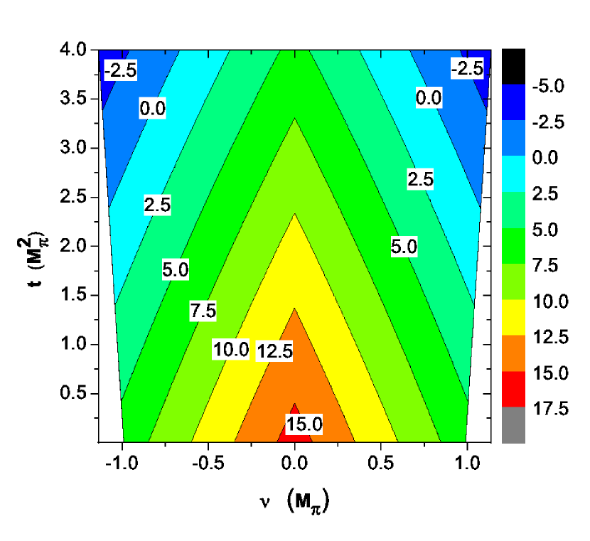
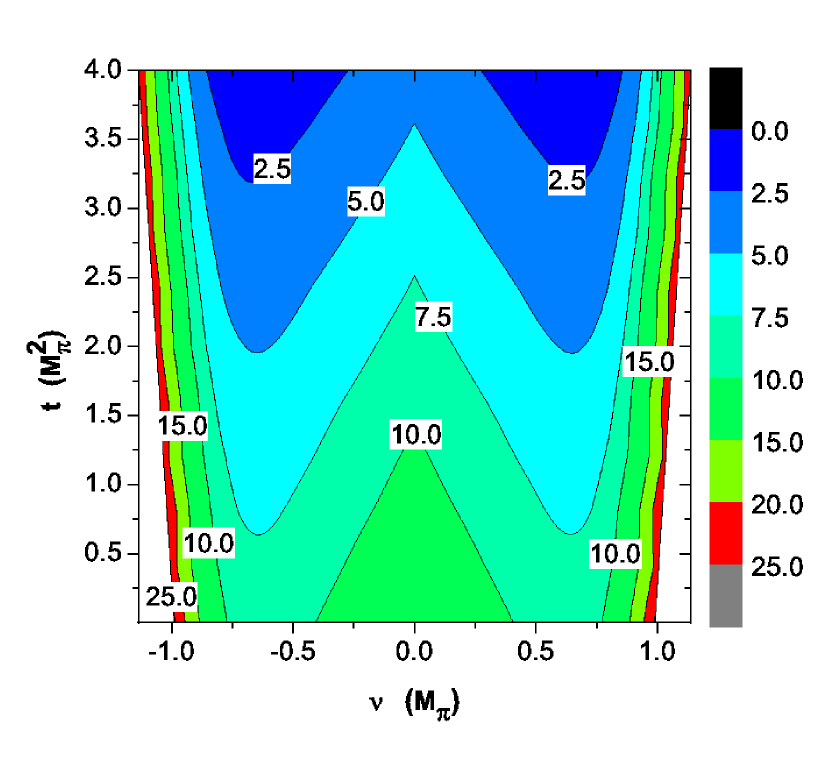
Figure 2: Positivity bound on LECs at $O(p^{3})$ level. The fit results from ‘Fit I-$O(p^{3})$’ given in Ref. yao are employed for plotting $f(\alpha,\nu,t)$ at ${\cal O}(p^{3})$. Left-hand side: only tree-level; right-hand-side: tree-level + loops. Similar results are obtained if one uses instead the ‘WI08’ results with $\not{\Delta}$-ChPT given in Ref. oller .

The scattering amplitudes in EOMS-B$\chi$PT were computed up to $O(p^{3})$ in Refs. oller and yao independently. Therein, the amplitudes were employed to perform fits to existing experimental phase-shift data , determining the concerning LECs. Here, the positivity constraints, displayed by Eq. (33), provide additional information about the amplitudes. When $n=2$, they turn into Eq. (34) and give bounds on the LECs at the $O(p^{3})$ level:

$$f(\alpha,\nu,t)\quad=\quad 4\alpha c_{2}-8(\alpha-1)m_{N}(d_{14}-d_{15})-h_{+}^{(2)}(\alpha,\nu,t)-\left|24\alpha\nu d_{3}-h_{-}^{(2)}(\alpha,\nu,t)\right|\geq 0\ ,\qquad\qquad(\nu,t)\in{\cal R}\,,$$ (36)

with $\alpha_{\rm min}(t)\leq\alpha\leq\alpha_{\rm max}(t)$ and the second derivatives of the non-pole loop contributions,

$$h_{\pm}^{(2)}(\alpha,\nu,t)=-F_{\pi}^{2}\frac{{\rm d}^{2}\tilde{D}^{\pm,{\rm loop}}_{\alpha}(\nu,t)}{{\rm d}\nu^{2}}\ .$$ (37)

Note that the left-hand side of Eq. (36) is a multivariate function with respect to $\alpha$, $\nu$ and $t$.

The inequality given by Eq. (36) is useful for judging the goodness of the fit results in Refs. oller and yao . In both of them the minimal value of $f(\alpha,\nu,t)$ is always achieved for $\alpha=\alpha_{\rm min}(t)$. After setting $\alpha=\alpha_{\rm min}(t)$, the scanning of $(\nu,t)$ within the region ${\cal R}$ yields the most stringent bound for $\nu=\pm 0.68M_{\pi},~{}t=4M_{\pi}^{2}$ in the ${\cal O}(p^{3})$ analysis yao , which is well respected: $f(\alpha_{\rm min}(4M_{\pi}^{2}),\pm 0.68M_{\pi},4M_{\pi}^{2})=0.83\geq 0$. In a similar way, the ${\cal O}(p^{3})$ analysis oller produces its most stringent bound for $\nu=\pm 0.65M_{\pi},~{}t=4M_{\pi}^{2}$ and $\alpha=\alpha_{\rm min}(4M_{\pi}^{2})$, which is well fulfilled: $f(\alpha_{\rm min}(4M_{\pi}^{2}),\pm 0.65M_{\pi},4M_{\pi}^{2})=1.03\geq 0$.

The contour plot for $f(\alpha,\nu,t)$ in the region ${\cal R}$, with $\alpha=\alpha_{\rm min}(t)$, is shown in Fig. 2. We used the LEC central values from Ref. yao . We noticed that at ${\cal O}(p^{3})$ the EOMS-scheme renormalized loop contributions were numerically relevant. If only the tree diagrams were considered in the inequality (34) the corresponding bound fails in some regions of $\mathcal{R}$, where $f(\alpha,\nu,t)<0$ (see the left-hand side graph in Fig. 2). Hence, the loop contribution is crucial. It is needed not only at the formal level for the consistence of the effective theory but also for the numerical fulfillment of the positivity constraints at this chiral order.

The analyses above were carried out with the central values of the LECs. In order to study the influence of the error and to provide a convenient inequality that can be used in future analysis, we take the particular point $\nu=\pm 0.68M_{\pi},~{}t=4M_{\pi}^{2},~{}\alpha=\alpha_{\rm min}(4M_{\pi}^{2})=0.85$, where the bound reads

$$f(\alpha,\nu,t)\quad=\quad 3.40c_{2}+1.11(d_{14}-d_{15})-0.29-|1.93d_{3}+1.22|\geq 0\ ,\qquad\qquad(\nu=\pm 0.68M_{\pi},~{}t=4M_{\pi}^{2},~{}\alpha=0.85)\ ,$$ (38)

with $c_{2}$ and the $d_{j}$ given in GeV^-1 and GeV^-2 units, respectively. Notice that the numerical coefficients in this equation do not depend on ${\cal O}(p^{2})$ or ${\cal O}(p^{3})$ LECs, and are fully determined by $m_{N}$, $M_{\pi}$, $g_{A}$ and $F_{\pi}$. Eq. (38) provides the optimal bound for Ref. yao and nearly the optimal for Ref. oller . Considering now the ${\cal O}(p^{2})$ and ${\cal O}(p^{3})$ LEC uncertainties in the previous ${\cal O}(p^{3})$ inequality one gets (in units of GeV^-1)

$$f(\alpha,\nu,t) = 5.42\pm 1.22-|-4.59\pm 0.98|\overset{?}{\geq}0\qquad\mbox{(Ref.~{}\cite[cite]{\@@bibref{Authors Phrase1YearPhrase2}{yao}{\@@citephrase{(}}{\@@citephrase{)}}}), }$$ (39)

$$f(\alpha,\nu,t) = 4.89\pm 1.23-|-3.84\pm 0.98|\overset{?}{\geq}0\qquad\mbox{(Ref.~{}\cite[cite]{\@@bibref{Authors Phrase1YearPhrase2}{oller}{\@@citephrase{(}}{\@@citephrase{)}}}).}$$ (40)

See Table 1 for details on the LECs oller ; yao . Here the formula $\Delta f=\sqrt{\sum_{i}\left[f^{\prime}(\overline{x}_{i})\Delta x_{i}\right]^{2}}$ is adopted to propagate the errors of the LECs, where $x_{i}$ stands for the LECs with $\overline{x}_{i}$ the central values and $\Delta x_{i}$ the corresponding errors. These expressions show a violation of the positivity constrains in part of the confidence region and queries the convergence of the pion-nucleon scattering amplitude at the $O(p^{3})$ level. Actually, this was first pointed out by Ref. oller where it was argued that the pion-nucleon calculation in EOMS scheme may have problems with the convergence of the chiral expansion. This is partly confirmed by the ${\cal O}(p^{3})$ positivity analysis shown here, where not all the values within the $1\sigma$ confidence intervals fulfill the bound. Thus, the constraint (38) may help to stabilize future fits to data and the chiral expansion.

Table 1: LECs involved in the positivity bounds without explicit $\Delta$(1232) contributions. Actually, the $c_{i}$ in the Fit I(a)-$O(p^{4})$ yao stand for $\hat{c}_{i}$. The $*$ denotes an input quantity. The $c_{i}$, $d_{j}$ and $e_{k}$ have units of GeV^-1, GeV^-2 and GeV^-3, respectively.

LEC	Fit I-$O(p^{3})$ yao	WI08 ($\not{\Delta}$-ChPT) oller	Fit I(a)-$O(p^{4})$ yao	Fit I(b)-$O(p^{4})$ yao	Fit I(c)-$O(p^{4})$ yao
$c_{1}$	$-1.39\pm 0.07$	$-1.50\pm 0.06$	$-1.08\pm 0.06$	$-1.39^{*}$	$-1.09\pm 0.08$
$c_{2}$	$4.01\pm 0.09$	$3.74\pm 0.09$	$2.78\pm 0.11$	$4.01^{*}$	$2.24\pm 0.05$
$c_{3}$	$-6.61\pm 0.08$	$-6.63\pm 0.08$	$-5.26\pm 0.14$	$-6.61^{*}$	$-5.05\pm 0.22$
$c_{4}$	$3.92\pm 0.04$	$3.68\pm 0.05$	$2.43\pm 0.19$	$3.92^{*}$	$2.43\pm 0.19$
$d_{3}$	$-3.02\pm 0.51$	$-2.63\pm 0.51$	$-6.87\pm 0.16$	$-8.04\pm 0.13$	$-6.87\pm 0.15$
$d_{14}-d_{15}$	$-7.15\pm 1.06$	$-6.80\pm 1.07$	$-12.09\pm 0.24$	$-13.90\pm 0.20$	$-11.94\pm 0.23$
$e_{15}$	$\cdots$	$\cdots$	$-14.99\pm 0.55$	$-14.50\pm 0.55$	$-5.41\pm 0.57$
$e_{16}$	$\cdots$	$\cdots$	$7.35\pm 0.35$	$7.65\pm 0.35$	$4.34\pm 0.28$
$e_{18}$	$\cdots$	$\cdots$	$6.07\pm 1.18$	$-0.79\pm 1.19$	$6.00\pm 1.26$
$e_{20}+e_{35}$	$\cdots$	$\cdots$	$\cdots$	$-12.86\pm 0.83$	$\cdots$
$e_{22}-4e_{38}$	$\cdots$	$\cdots$	$\cdots$	$-8.19\pm 1.79$	$\cdots$

V.2 Analysis at $O(p^{4})$ level

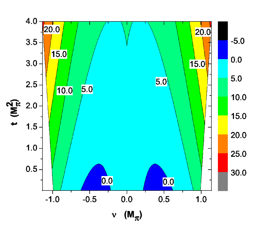
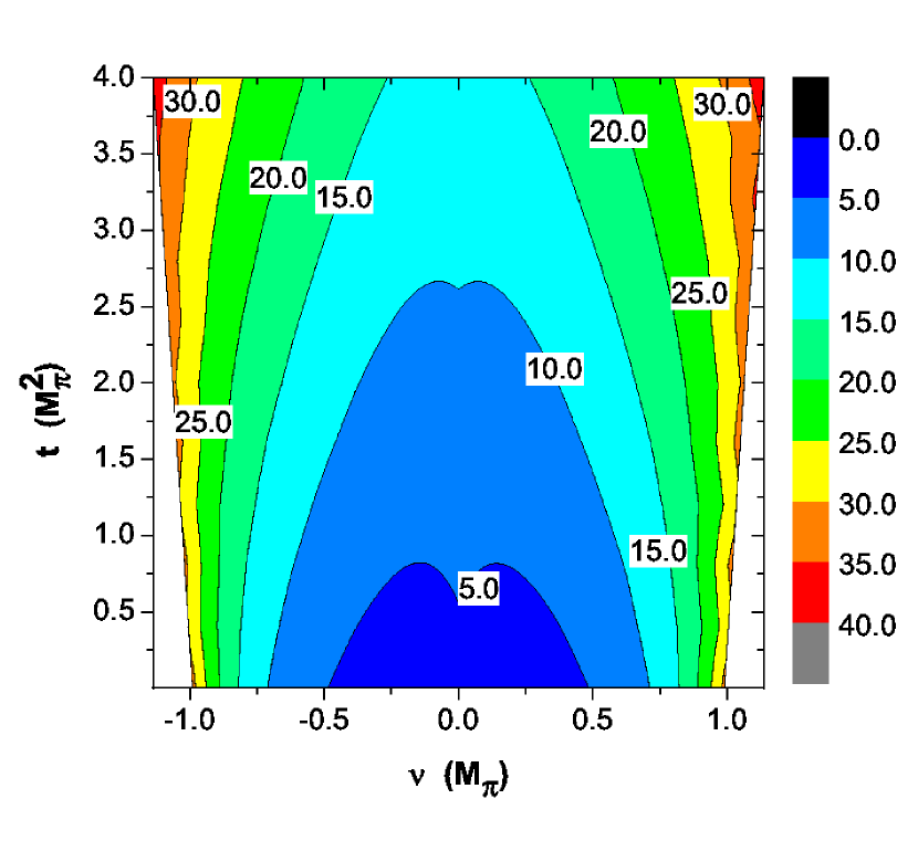
Figure 3: Positivity bound on LECs at $O(p^{4})$ level. The fit results from ‘Fit I(a)-$O(p^{4})$’ given in Ref. yao are employed for plotting $f(\alpha,\nu,t)$ up to ${\cal O}(p^{4})$ in EOMS-B$\chi$PT. Left-hand side: only tree-level; right-hand side: tree+loop

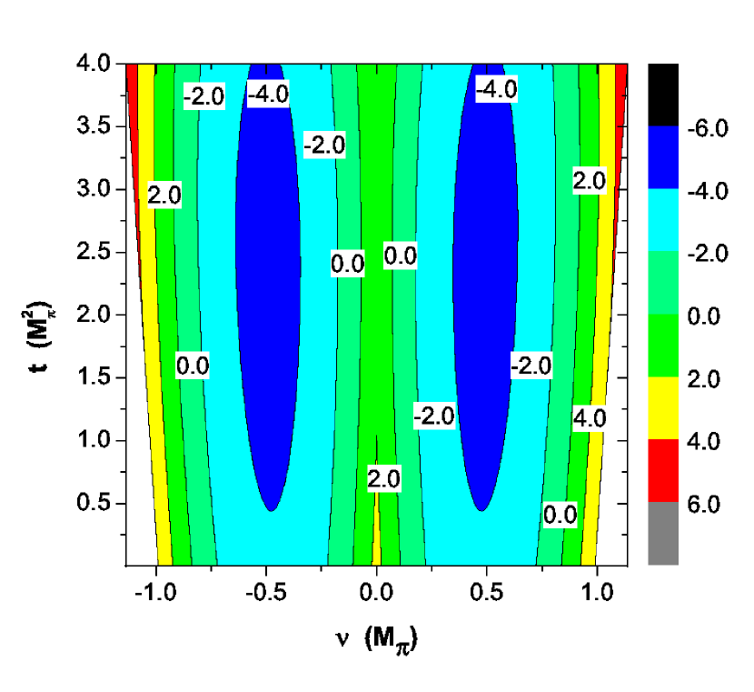
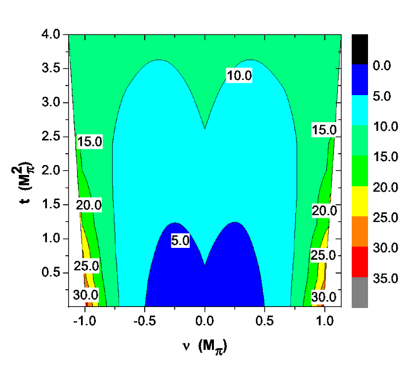
Figure 4: Positivity bound on LECs at $O(p^{4})$ level. The fit results from ‘Fit I(b)-$O(p^{4})$’ given in Ref. yao are employed for plotting $f(\alpha,\nu,t)$ up to ${\cal O}(p^{4})$ in EOMS-B$\chi$PT. Left-hand side: only tree-level; right-hand side: tree+loop

At the $O(p^{4})$ level, with two subtractions ($n=2$), the bound (34) on the LECs turns into

$$f(\alpha,\nu,t)\quad=\quad 4\alpha\hat{c}_{2}-8(\alpha-1)m_{N}(d_{14}-d_{15})+32\alpha\left[-\hat{c}_{1}\hat{c}_{2}M_{\pi}^{2}-2e_{15}m_{N}\nu_{B}+6e_{16}\nu^{2}\right]-h_{+}^{(2)}(\alpha,\nu,t)$$

$$\qquad\qquad\qquad\qquad\qquad-\left|24\alpha\nu d_{3}-96(\alpha-1)e_{18}m_{N}\nu-h_{-}^{(2)}(\alpha,\nu,t)\right|\geq 0\ ,$$ (41)

where $\hat{c}_{1}=c_{1}-2M_{\pi}^{2}(e_{22}-4e_{38})$ and $\hat{c}_{2}=c_{2}+8M_{\pi}^{2}(e_{20}+e_{35})$ yao . Here the non-pole loop terms $h_{\pm}^{(2)}(\alpha,\nu,t)$ contain both $O(p^{3})$ and $O(p^{4})$ contributions. It is useful to reexpress the bound (V.2) up to ${\cal O}(p^{4})$ as

$$f(\alpha,\nu,t)\quad=\quad 4\alpha c_{2}-8(\alpha-1)m_{N}(d_{14}-d_{15})+32\alpha\left[(e_{20}+e_{35}-c_{1}c_{2})M_{\pi}^{2}-2e_{15}m_{N}\nu_{B}+6e_{16}\nu^{2}\right]-h_{+}^{(2)}(\alpha,\nu,t)$$

$$\qquad\qquad\qquad\qquad\qquad-\left|24\alpha\nu d_{3}-96(\alpha-1)e_{18}m_{N}\nu-h_{-}^{(2)}(\alpha,\nu,t)\right|\geq 0\ .$$ (42)

These two equations differ from each other by terms of ${\cal O}(p^{5})$ in the chiral expansion or higher.

Two different strategies were adopted in Ref. yao to perform fits to the pion-nucleon phase-shift and to determine the various LECs at $O(p^{4})$ level within EOMS-B$\chi$PT. The strategy called ‘Fit I(a)-$O(p^{4})$’ provides values for the LECs in Eq. (V.2), and the other one, called ‘Fit I(b)-$O(p^{4})$’, gives values for the LECs in Eq. (V.2). As it happened before at ${\cal O}(p^{3})$, the function $f(\alpha,\nu,t)$ up to ${\cal O}(p^{4})$ also achieves its minimal values for $\alpha=\alpha_{\rm min}(t)$. For the central values of the LECs (see Table 1), the ${\cal O}(p^{4})$ contour plot for $f(\alpha,\nu,t)$ in the region ${\cal R}$, with $\alpha=\alpha_{\rm min}(t)$, are shown in Figs. 3 and 4 .These two figures correspond to the two different ${\cal O}(p^{4})$ analysis, ’Fit I(a)-${\cal O}(p^{4})$’ yao in Eq. (V.2) and ’Fit I(b)-${\cal O}(p^{4})$’ yao in Eq. (V.2), respectively. The most stringent bound stemming from Eq. (V.2) takes the form

$$f(\alpha,\nu,t)\quad=\quad 4.36\hat{c}_{2}\,\,\,-\,\,\,2.74-0.23\hat{c}_{1}-0.23\hat{c}_{3}+0.14\hat{c}_{4}+0.11e_{16}+0.62(e_{15}-\hat{c}_{1}\hat{c}_{2})$$

$$\qquad\qquad\qquad\qquad-|0.18-0.26\hat{c}_{1}-0.07\hat{c}_{2}-0.24\hat{c}_{3}+0.20\hat{c}_{4}+0.57d_{3}|\quad\geq\quad 0\ ,\qquad\quad(\nu=\pm 0.17M_{\pi},~{}t=0,~{}\alpha=\alpha_{\rm min})\ ,$$

with the $c_{i}$, $d_{j}$ and $e_{k}$ in units of GeV^-1, GeV^-2 and GeV^-3, respectively. Substituting the LECs in Eq. (V.2) with the values from ‘Fit I(a)-$O(p^{4})$’ yao (see Table 1), one finds (in units of GeV^-1)

$$f(\alpha,\nu,t) = 4.56\pm 0.66-|-1.88\pm 0.11|\geq 0\,,$$ (44)

where the positivity constraint is definitely well obeyed at the $O(p^{4})$ level in the chiral expansion.

In the alternative ${\cal O}(p^{4})$ form (V.2) the most stringent bound reads

$$f(\alpha,\nu,t)\quad=\quad 4.36c_{2}\,\,\,-\,\,\,2.72-0.23c_{1}-0.23c_{3}+0.14c_{4}+0.11e_{16}+0.62(e_{15}+e_{20}+e_{35}-c_{1}c_{2})$$

$$\qquad\qquad\qquad\qquad-|0.19-0.27c_{1}-0.08c_{2}-0.26c_{3}+0.21c_{4}+0.60d_{3}|\geq 0\ ,\qquad\qquad(\nu=\pm 0.18M_{\pi},~{}t=0,~{}\alpha=\alpha_{\rm min})\ ,$$

with the $c_{i}$, $d_{j}$ and $e_{k}$ in units of GeV^-1, GeV^-2 and GeV^-3, respectively. Substituting the values from ‘Fit I(b)-$O(p^{4})$’ yao in Table 1, we find that the positivity bound is again well respected at $O(p^{4})$:

$$f(\alpha,\nu,t) = 4.61\pm 0.62-|-2.04\pm 0.08|\geq 0\,,$$ (46)

given in units of GeV^-1.

As it happened at ${\cal O}(p^{3})$, our ${\cal O}(p^{4})$ analyses in Figs. 3 and 4 (left-hand side) show that in the EOMS scheme the bounds are violated in some regions of $\mathcal{R}$ if only the (renormalized) tree-level amplitude is included; loops play an important role, both at $O(p^{3})$ and $O(p^{4})$.

V.3 Comparison at special subthreshold points

At the subthreshold region, some famous low-energy theorems can be established at particular points: the Cheng-Dashen (CD) point $(\nu=0,\,t=2M_{\pi}^{2})$ CDpoint and the Adler point $(\nu=0,\,t=M_{\pi}^{2}$) Adlerpoint . The positivity bound is found to be very clearly obeyed at these points, both at $O(p^{3})$ and $O(p^{4})$ (see Figs 2-4). Nonetheless , it is still interesting to study the evolution of the constraints at these points as the chiral order increases from $O(p^{3})$ to $O(p^{4})$. A priori, the variation of the bounds at the CD and Adler points should not be too large, since the chiral convergence of the amplitudes is expected to be good ($\nu\ll m_{N}$ and $t\ll m_{N}^{2}$) and these points are far away from non-analytical points. On the other hand, the bounds near threshold always get large values for $f(\alpha,\nu,t)$ and suffer a sizable variation from one chiral order to another as the derivatives of the loop amplitude may diverge at threshold. In what follows, the bounds at these special subthreshold points will be calculated with the condition $\alpha=\alpha_{\rm min}(t)$, where we extracted the most stringent bounds in the sections above.

At the CD point, where $(\nu=0,\,t=2M_{\pi}^{2})$, setting $\alpha=\alpha_{\rm min}(2M_{\pi}^{2})$ the $O(p^{3})$ bound (36) reads (in units of GeV^-1)

$$f(\alpha_{\rm min}(2M_{\pi}^{2}),0,2M_{\pi}^{2})^{{\cal O}(p^{3})}\quad=\quad\left\{\begin{array}[]{ll}8.7\,,&\quad\hbox{for `Fit I-$O(p^{3})$' from Ref.~{}\cite[cite]{\@@bibref{Authors Phrase1YearPhrase2}{yao}{\@@citephrase{(}}{\@@citephrase{)}}},}\\ 7.9\,,&\quad\hbox{for `WI08' of $\not{\Delta}$-ChPT from Ref.~{}\cite[cite]{\@@bibref{Authors Phrase1YearPhrase2}{oller}{\@@citephrase{(}}{\@@citephrase{)}}},}\end{array}\right.$$ (49)

and the $O(p^{4})$ bounds (V.2) and (V.2) become now (in units of GeV^-1)

$$f(\alpha_{\rm min}(2M_{\pi}^{2}),0,2M_{\pi}^{2})^{{\cal O}(p^{4})}=\left\{\begin{array}[]{ll}8.5\,,&\quad\hbox{for `Fit I(a)-$O(p^{4})$' from~{}\cite[cite]{\@@bibref{Authors Phrase1YearPhrase2}{yao}{\@@citephrase{(}}{\@@citephrase{)}}},}\\ 8.5\,,&\hbox{for `Fit I(b)-$O(p^{4})$' from~{}\cite[cite]{\@@bibref{Authors Phrase1YearPhrase2}{yao}{\@@citephrase{(}}{\@@citephrase{)}}}.}\end{array}\right.$$ (52)

As expected, the $O(p^{3})$ bounds at the CD point, located at the center of the upper part $\mathcal{R}$ of the Mandelstam triangle, suffer small variations when taking the EOMS-B$\chi$PT up to $O(p^{4})$.

In a similar way, taking the optimal value $\alpha=\alpha_{\rm min}(M_{\pi}^{2})$, the $O(p^{3})$ bound (36) at the Adler point $(\nu=0,\,t=M_{\pi}^{2})$ reads (in units of GeV^-1)

$$f(\alpha_{\rm min}(M_{\pi}^{2}),0,M_{\pi}^{2})^{{\cal O}(p^{3})}\quad=\quad\left\{\begin{array}[]{ll}11.0\,,&\quad\hbox{for `Fit I-$O(p^{3})$' from Ref.~{}\cite[cite]{\@@bibref{Authors Phrase1YearPhrase2}{yao}{\@@citephrase{(}}{\@@citephrase{)}}},}\\ 10.0\,,&\hbox{for `WI08' of $\not{\Delta}$-ChPT from Ref.~{}\cite[cite]{\@@bibref{Authors Phrase1YearPhrase2}{oller}{\@@citephrase{(}}{\@@citephrase{)}}},}\end{array}\right.$$ (55)

and the $O(p^{4})$ bounds (V.2) and (V.2) give (in units of GeV^-1)

$$f(\alpha_{\rm min}(M_{\pi}^{2}),0,M_{\pi}^{2})^{{\cal O}(p^{4})}\quad=\quad\left\{\begin{array}[]{ll}6.1\,,&\hbox{for `Fit I(a)-$O(p^{4})$' from~{}\cite[cite]{\@@bibref{Authors Phrase1YearPhrase2}{yao}{\@@citephrase{(}}{\@@citephrase{)}}},}\\ 6.0\,,&\hbox{for `Fit I(b)-$O(p^{4})$' from~{}\cite[cite]{\@@bibref{Authors Phrase1YearPhrase2}{yao}{\@@citephrase{(}}{\@@citephrase{)}}}.}\end{array}\right.$$ (58)

Compared to the CD point, the variation of the bound at the Adler point is slightly larger, yet still rather acceptable.

V.4 Analysis including the $\Delta(1232)$

Table 2: LECs involved in the positivity bounds with explicit $\Delta$(1232) contribution. The $*$ denotes an input quantity. The $c_{i}^{\prime}$, $d_{j}^{\prime}$ and $e_{k}^{\prime}$ have units of GeV^-1, GeV^-2 and GeV^-3 respectively, and $h_{A}$ is dimensionless.

LEC	Fit II-$O(p^{3})$ yao	WI08 ($\Delta$-ChPT) oller	Fit II(a)-$O(p^{4})$ yao	Fit II(b)-$O(p^{4})$ yao	Fit II(c)-$O(p^{4})$ yao
$c_{1}^{\prime}$	$-0.81\pm 0.03$	$-1.00\pm 0.04$	$-1.03\pm 0.03$	$-0.81^{*}$	$-0.95\pm 0.05$
$c_{2}^{\prime}$	$1.46\pm 0.09$	$1.01\pm 0.04$	$0.50\pm 0.04$	$1.46^{*}$	$0.10\pm 0.06$
$c_{3}^{\prime}$	$-3.10\pm 0.12$	$-3.04\pm 0.02$	$-3.17\pm 0.05$	$-3.10^{*}$	$-2.64\pm 0.08$
$c_{4}^{\prime}$	$2.35\pm 0.06$	$2.02\pm 0.01$	$0.79\pm 0.03$	$2.35^{*}$	$0.80\pm 0.03$
$d_{3}^{\prime}$	$-0.47\pm 0.05$	$-0.23\pm 0.27$	$-5.04\pm 0.05$	$-4.75\pm 0.04$	$-4.90\pm 0.04$
$d_{14}^{\prime}-d_{15}^{\prime}$	$-0.90\pm 0.15$	$-0.50\pm 0.50$	$-5.61\pm 0.09$	$-5.82\pm 0.09$	$-5.58\pm 0.09$
$e_{15}^{\prime}$	$\cdots$	$\cdots$	$5.05\pm 0.13$	$15.29\pm 0.12$	$10.52\pm 0.12$
$e_{16}^{\prime}$	$\cdots$	$\cdots$	$-0.31\pm 0.07$	$-2.76\pm 0.07$	$-1.50\pm 0.05$
$e_{18}^{\prime}$	$\cdots$	$\cdots$	$-10.99\pm 0.12$	$-11.58\pm 0.11$	$-9.87\pm 0.12$
$e_{20}^{\prime}+e_{35}^{\prime}$	$\cdots$	$\cdots$	$\cdots$	$-13.12\pm 0.28$	$\cdots$
$e_{22}^{\prime}-4e_{38}^{\prime}$	$\cdots$	$\cdots$	$\cdots$	$10.29\pm 0.82$	$\cdots$
$h_{A}$	$2.82\pm 0.04$	$2.87\pm 0.04$	$2.90^{*}$	$2.90^{*}$	$2.90^{*}$

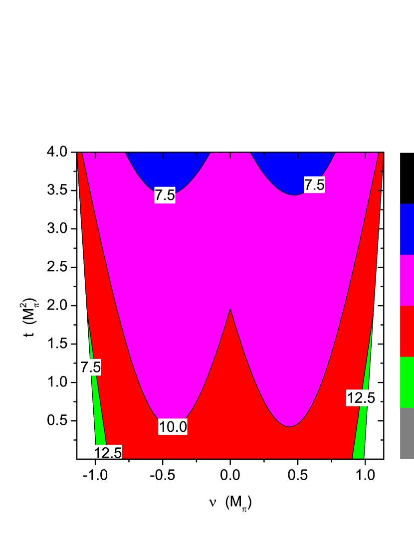
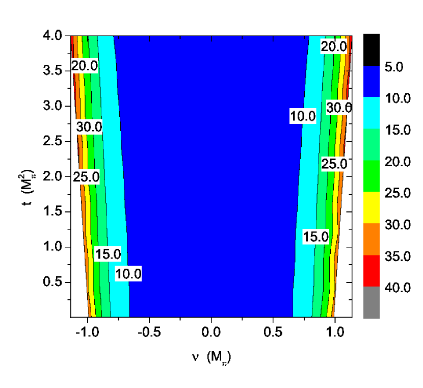
Figure 5: Positivity bound on LECs at $O(p^{3})$ level including the $\Delta(1232)$. The fit results from ‘Fit II-$O(p^{3})$’ given in Ref. yao are employed for plotting $f(\alpha,\nu,t)$. Left-hand side: only tree-level; right-hand side: tree+loop. The analysis ‘WI08’ with $\Delta$-ChPT in Ref. oller yields a similar outcome.

In Refs. oller ; yao , the contribution from the $\Delta(1232)$ was explicitly included to describe the phase-shift up to center-of-mass energies of $1.20$ GeV. The corresponding LECs were pinned down through fits to the experimental data. the value of $f(\alpha,\nu,t)$ can be readily obtained from the EOMS-B$\chi$PT bounds at ${\cal O}(p^{3})$ (Eq. (36)) and ${\cal O}(p^{4})$ (Eqs. (V.2) and (V.2)) by conveniently adding the corresponding contributions $F_{\pi}^{2}\frac{d^{2}}{d\nu^{2}}\tilde{D}^{\pm}_{\alpha}(\nu,t)|^{\rm\Delta-Born}$. In addition, at ${\cal O}(p^{4})$ in the $\delta$ counting Pascalutsa one may have contributions from $\Delta$ resonance loops and the ${\cal O}(p^{2})$ LECs in the one-loop diagrams need to be modified (see App. A.2 in Ref. yao ). The contour plots for $f(\alpha,\nu,t)$ inside the upper part of the Mandelstam triangle for the $O(p^{3})$ amplitude including the $\Delta(1232)$ is shown in Fig. 5. Here we provided the fit results from ‘Fit II-$O(p^{3})$’ yao . The ‘WI08’ analysis in Ref.oller produces similar results. The ${\cal O}(p^{3})$ calculations oller ; yao took the $\Delta$(1232) into consideration by adding the leading $\Delta$–Born term contribution explicitly (see the Appendices therein). We find that this leading $\Delta$–Born term provides a definite positive and large contribution to the $O(p^{3})$ bounds (see Fig. 5), and both the tree-level and the full (tree+loop) bound are well obeyed.

At $O(p^{4})$, the leading order Born contribution from explicit $\Delta$(1232) exchanges were considered in Ref. yao and the $\Delta$(1232) loop contributions were also partially included. Therein, two scenarios were carried out, “Fit II(a)” and “Fit II(b)”, corresponding to the two different ways of writing down the ${\cal O}(p^{4})$ part shown in Eqs. (V.2) and (V.2), but now including explicitly the $\Delta(1232)$. At the ${\cal O}(p^{4})$ chiral order one needs to take into account the $\Delta$ resonance loops. Their ${\cal O}(p^{4})$ contribution was accounted in Ref. yao by adding the $\Delta$ contributions $c_{1}^{\Delta}=0$, $c_{2}^{\Delta}=-c_{3}^{\Delta}=2c_{4}^{\Delta}=h_{A}^{2}m_{N}^{2}/[9m_{\Delta}^{2}(m_{\Delta}-m_{N})]$ to the ${\cal O}(p^{2})$ parameters $c_{k}$ present in the ${\cal O}(p^{4})$ B$\chi$PT loop . Fig. 6 shows the $f(\alpha,\nu,t)$ contour plot for “Fit II(a)”, having “Fit II(b)” a similar structure. The left-hand side graph in Fig. 6 presents the contour plots if only the tree-level amplitude is taken into account, while the right-hand side shows the full bounds (tree+loop).

It is shocking that both the tree-level and full bounds are largely violated in the upper left and right corners of the region $\mathcal{R}$. The violation of the positivity bounds implies a possible issue in the $O(p^{4})$ fit results with the $\Delta$(1232) in Ref. yao . To have a better understanding of this violation, one should pay attention to the unusual approach, shown in Appendix A.2 in Ref. yao , to include the $\Delta$-contained loop Feynman Diagrams. With this approach, the propagators of $\Delta$(1232) occurring in the loops are integrated out, which corresponds to an expansion with respect to $1/m_{\Delta}$. The expansion leads to a polynomial of $1/m_{\Delta}$, namely the analytic structure proportional to $\ln m_{\Delta}$ will never appear in the scattering amplitude. A direct and convenient way to compensate the contribution from $\ln m_{\Delta}$ terms is to adjust the values of the LECs of the tree amplitudes, since they are chiral polynomials. Actually, compared to the $O(p^{4})$ fits without $\Delta$, the LECs of $O(p^{4})$ in fits with $\Delta$ change a lot, especially in the case of $e_{18}$. Moreover, the violation of the positivity bound is mainly caused by $e_{18}$. When the energy goes larger, bigger changes of LECs occur, possibly leading to positivity violation. Hence, the above approach of including $\Delta$-contained loops may be practical at low energies but invalid at high energies. However, no one knows at which energy the approach fails, as the exact full expression of the $\Delta$-contained loop amplitude is unknown. Nevertheless, the positivity bounds can tell us something. Here, the violation of the bounds shown in Figs. 6 indicates that the approach fails beyond 1.2 GeV, deserving further calculations of the exact $\Delta$-contained loop amplitudes.

To conclude, at $O(p^{3})$ level, both the tree-level and full bounds with $\Delta$ contribution are well satisfied, since the leading Born term of $\Delta$ gives a large and positive contribution. At $O(p^{4})$ level, the bounds are badly violated, which might be mainly due to the unusual way of including the $\Delta$-contained loop contribution. The violation indicates that a further exact and full calculation of the $\Delta$-contained loop is necessary when performing fits beyond the energy of 1.2 GeV in the center of mass frame.

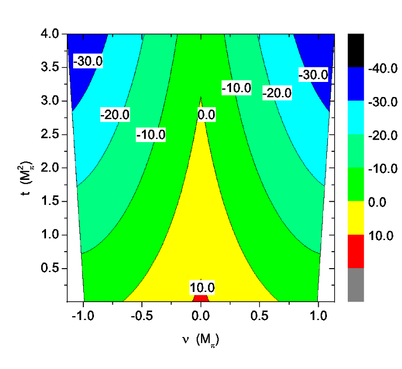
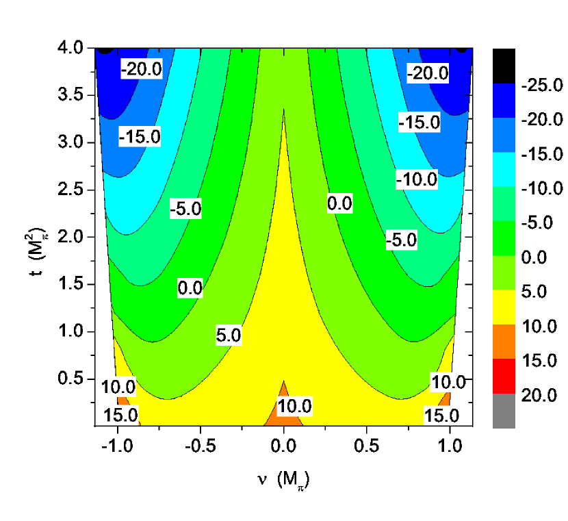
Figure 6: Positivity bound on LECs at $O(p^{4})$ level. The fit results from ‘Fit II(a)-$O(p^{4})$’ given in Ref. yao are employed for plotting $f(\alpha,\nu,t)$. Left-hand side: only tree-level; right-hand side: tree+loop. Similar results are found with ‘Fit II(b)-$O(p^{4})$’ from Ref. yao .

Finally, we would also like to discuss the impact of these constraints on the values of the pion-nucleon sigma term, $\sigma_{\pi N}$, analyzed in Ref. yao . Therein, the lattice QCD data for $m_{N}$ and the pion-nucleon scattering data were employed to determine the pion-nucleon sigma term. As a consequence of this, two different results were reported: $\sigma_{\pi N}=52\pm 7$ MeV (’Fit I(c)-${\cal O}(p^{4})$’ without $\Delta(1232)$) and $\sigma_{\pi N}=45\pm 6$ MeV (’Fit II(c)-${\cal O}(p^{4})$’ with explicit $\Delta(1232)$ contributions). However, though compatible, one may wonder which value is more accurate and carries less theoretical uncertainties. The positivity bounds derived in this work may provide an answer to this. The values from “Fit I(c)-$O(p^{4})$” and “Fit II(c)-$O(p^{4})$” for the LECs involved in the bounds are listed in Tabs. 1 and 2, respectively. The contour plots for the positivity bounds, without and with explicit $\Delta$ contribution, are shown in Figs. 7. As we can see, the bound with $\Delta$ contribution are violated in most of the region ${\cal{R}}$, while the one without explicit $\Delta$ contribution are well satisfied. This may imply that the value $\sigma_{\pi N}=52\pm 7$ MeV is more reasonable than $\sigma_{\pi N}=45\pm 6$ MeV. Again we owe this to the lack of an exact calculation of the $\Delta$-contained loop.

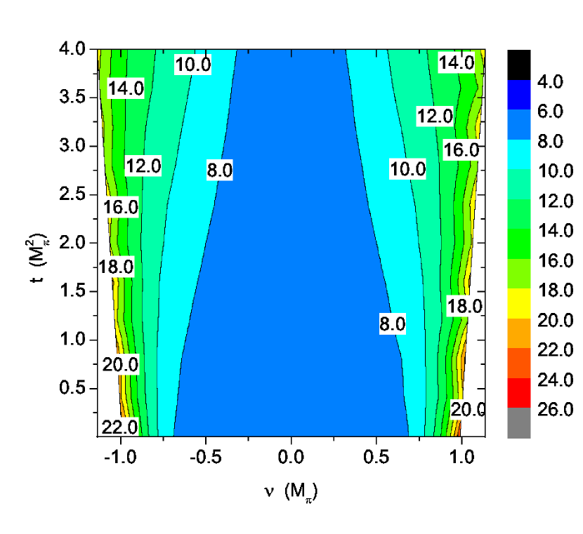
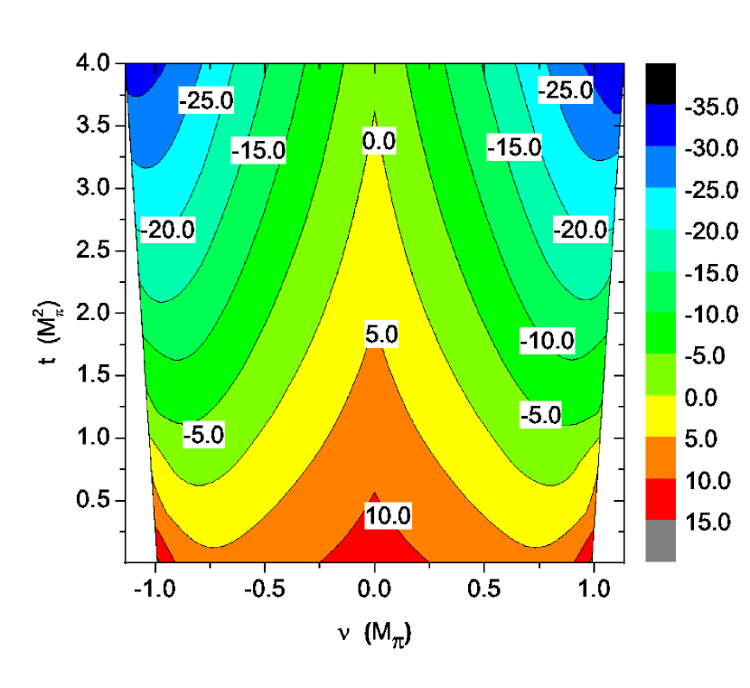
Figure 7: Positivity bound on LECs at $O(p^{4})$ level. The fit results from ‘Fit I(c)-$O(p^{4})$’ and ‘Fit II(c)-$O(p^{4})$’ given in Ref. yao are employed for plotting $f(\alpha,\nu,t)$. Left-hand side: full bound without explicit $\Delta$ contribution; right-hand side: full bound with explicit $\Delta$ contribution.

VI Conclusions

Using the general S-matrix arguments, such as analyticity, crossing symmetry and unitarity, we derived positivity constraints on the pion-nucleon scattering amplitudes $D_{\alpha}(\nu,t)=\alpha A(\nu,t)+\nu B(\nu,t)$ in the upper part of Mandelstam triangle, ${\cal R}$. These constraints are further changed into positivity bounds on the chiral LECs of the pion-nucleon Lagrangian both at $O(p^{3})$ and $O(p^{4})$ level. In combination with the central values of the LECs from Refs. yao ; oller within EOMS-B$\chi$PT, it is found that the bounds at tree level are always violated in some regions inside ${\cal R}$, while the full bounds (tree+loop) are well respected both for $O(p^{3})$ and $O(p^{4})$ analyses; loops are important and, in the chosen renormalization scheme (EOMS), they produce contributions to the positivity bound numerically of the same order as the tree-level diagrams.

Nonetheless, when considering the LEC uncertainties, the full and most stringent bounds at $O(p^{3})$ level are slightly violated in some parts of the $1\sigma$ intervals, pointing out the break down of EOMS-B$\chi$PT for those LEC values. However, this problem disappears the analysis is taken up to $O(p^{4})$, where the most stringent bounds are well obeyed in the full error interval.

We have provided the constraints for special points where the bounds are nearly optimal in terms of just a few ${\cal O}(p^{2})$, ${\cal O}(p^{3})$ and ${\cal O}(p^{4})$ LECs (depending on the chiral order one works at). We hope these positivity conditions can be easily implemented and employed to constrain future B$\chi$PT analyses.

Finally, the positivity bounds with an explicit $\Delta$ resonance have been also studied. The $\Delta$ Born-term provides a positive-definite contribution to the bounds and hence the bounds at $O(p^{3})$ level in the $\delta$-counting rule (see Ref. Pascalutsa ) are well satisfied. However, at the $O(p^{4})$ level, the bounds are violated when just a part of the $\Delta$ loops is included. We think that a complete one-loop calculation including $\Delta$–loops will solve this issue.

Appendix A Positive definite spectral function for $D_{\alpha}^{I}$

The dispersion relation for the analysis of the subthreshold amplitude is used to extract the positivity constraints. Hence a positive definite spectral function in the physical region $s\geq s_{\rm th}$ is required. Starting from Eqs. (15) and (16), one can immediately construct a preliminary combination of the form

$$0\,\leq\,{\rm Im}\bigg{\{}\alpha_{1}A^{I}(s,t)+\alpha_{2}B^{I}(s,t)\bigg{\}}\,=\,\vec{\alpha}^{\,\,T}\,\cdot\,{\rm Im}\vec{\cal A}^{I}(s,t)\,,\qquad\qquad{\rm where}\quad\vec{\alpha}=\left(\begin{array}[]{c}\alpha_{1}\\ \alpha_{2}\end{array}\right)\,.$$ (61)

Notice that in principle there is no restriction to the possible combinations we may consider, so one may consider combinations where $\vec{\alpha}$ depends also on $s$ and $t$ or, conversely, on $\nu$ and $\nu_{B}$. The only necessary condition will be that they are analytical functions in the $\nu$–integration domain in our fixed–t dispersion relation, i.e., they are real and do not contain discontinuities for $\nu\geq\nu_{th}$ for fixed t. Thus, for later convenience we will rather write the general combination of $A^{I}$ and $B^{I}$ in the form

$$0\,\leq\,\mbox{Im}\bigg{\{}\alpha_{1}A^{I}(s,t)+\alpha_{2}\nu B^{I}(s,t)\bigg{\}}\,=\,\vec{\alpha}^{\,\,T}\,\cdot\,\mbox{Im}\vec{\cal A}^{I}(s,t)\,,\qquad\qquad\mbox{{with} }\vec{\alpha}=\left(\begin{array}[]{c}\alpha_{1}\\ \alpha_{2}\nu\end{array}\right)\,,$$ (64)

where we introduced the $\nu$ factor in the $B^{I}(s,t)$ term. From now on we will use the notation

$$D^{I}_{\alpha}(s,t) \equiv \vec{\alpha}^{\,\,T}\,\cdot\,\vec{\mathcal{A}}^{I}(s,t)\,.$$ (65)

For the study of the positivity of Im$D_{\alpha}^{I}$ we will make use of the positivity of each PW, i.e., Im$f^{I}_{k}(s)\geq 0$ for $s\geq s_{th}$. Thus, we have that

$$0\,\leq\,\mbox{Im}D_{\alpha}^{I}(s,t)\, = \,\vec{\alpha}^{\,\,T}\,\cdot\,\sum_{\ell=0}^{\infty}S^{\ell}(s,t)\,\mbox{Im}\vec{\cal F}^{I}(s)$$ (66)

$$=\sum_{\ell=0}^{\infty}\vec{\alpha}^{\,\,T}\,S^{\ell}(s,t)\,\mbox{Im}\vec{\cal F}^{I}(s)$$

$$=\sum_{\ell=0}^{\infty}\bigg{(}\,\vec{\alpha}^{\,\,T}\vec{v}_{1}^{\,\,\ell}\,,\,\vec{\alpha}^{\,\,T}\vec{v}_{2}^{\,\,\ell}\,\bigg{)}\,\mbox{Im}\vec{\cal F}^{I}(s)\,.$$

For convenience, here the $2\times 2$ matrix $S^{\ell}(s,t)$ has been written in terms of two dimension–2 vectors:

$$S^{\ell}(s,z_{s})=\bigg{(}\,\vec{v}_{1}^{\,\,\ell}\,,\,\vec{v}_{2}^{\,\,\ell}\,\bigg{)}\,.$$ (67)

Hence the positivity of Im$f^{I}_{k}(s)$ ensures the positivity of Im$D_{\alpha}(s,t)$ whenever

$$\vec{\alpha}^{\,\,T}\vec{v}_{1}^{\,\,\ell}\geq 0\,,\qquad\qquad\vec{\alpha}^{\,\,T}\vec{v}_{2}^{\,\,\ell}\geq 0\,,$$ (68)

for $s\geq s_{th}$. The explicit form of these constraints is given by

$$\frac{4\pi}{E^{2}-m_{N}^{2}}\bigg{(}\,c_{11}(s,t)\,\alpha_{1}\,+\,c_{12}(s,t)\,\nu\,\alpha_{2}\bigg{)}\,\geq\,0\,,$$

$$-\,\frac{4\pi}{E^{2}-m_{N}^{2}}\bigg{(}\,c_{21}(s,t)\,\alpha_{1}\,+\,c_{22}(s,t)\,\nu\,\alpha_{2}\bigg{)}\,\geq\,0\,,$$ (69)

with

$$c_{11} = \frac{1}{2W}\bigg{[}(W+m_{N})(W-W_{+})(W-W_{-})P^{\prime}_{\ell+1}(z_{s})\,+\,(W-m_{N})(W+W_{+})(W+W_{-})P^{\prime}_{\ell}(z_{s})\bigg{]}\,,$$

$$c_{12} = (E-m_{N})P^{\prime}_{\ell+1}(z_{s})\,-\,(E+m_{N})P^{\prime}_{\ell}(z_{s})\,,$$

$$c_{21} = \frac{1}{2W}\bigg{[}(W+m_{N})(W-W_{+})(W-W_{-})P^{\prime}_{\ell}(z_{s})\,+\,(W-m_{N})(W+W_{+})(W+W_{-})P^{\prime}_{\ell+1}(z_{s})\bigg{]}\,,$$

$$c_{22} = (E-m_{N})P^{\prime}_{\ell}(z_{s})\,-\,(E+m_{N})P^{\prime}_{\ell+1}(z_{s})\,,$$

and the kinematical variables,

$$z_{s}(t,s)=1+\frac{\displaystyle t}{\displaystyle 2\vec{q}^{\,\,2}}\,,\qquad\qquad|\vec{q}|=\sqrt{\frac{\displaystyle\lambda(s,M_{\pi}^{2},m_{N}^{2})}{\displaystyle 4s}}\,,$$

$$W=\sqrt{s}\,,\qquad\qquad E=\sqrt{\vec{q}^{\,\,2}+m_{N}^{2}}=\frac{\displaystyle W^{2}+m_{N}^{2}-M_{\pi}^{2}}{\displaystyle 2W}\,,$$

$$W_{\pm}^{2}=(m_{N}\pm M_{\pi})^{2}\,,\qquad\qquad s_{th}=s_{+}\,,$$ (71)

with $\vec{q}$ being the three-momentum of the pion in the center-of-mass rest-frame.

Since $E\geq m_{N}$ when $s\geq s_{th}$ we can simplify the inequalities in the form

$$c_{11}\,\alpha_{1}\,+\,c_{12}\,\nu\,\alpha_{2}\,\geq\,0\,,$$

$$c_{21}\,\alpha_{1}\,+\,c_{22}\,\nu\,\alpha_{2}\,\leq\,0\,.$$ (72)

The coefficients $c_{mn}$ are combinations of the first derivative of the Legendre polynomials and in general the sign may change from one partial wave $\ell$ to another $\ell^{\prime}$, or from an energy $(s,t)$ to another. However, when $z_{s}(s,t)\geq 1$, i.e., when $t\geq 0$ for $s\geq s_{th}$, one has that $P^{\prime}_{k}(z_{s})\geq 0$ and then

$$c_{11}\geq 0\,,\qquad c_{21}\geq 0\,,$$ (73)

for any $s\geq s_{th}$ and $t\geq 0$ (as $W\geq m_{N}\geq 0$ and $W\geq W_{\pm}>0$). Thus, the inequalities get simplified into the form

$$\alpha_{1}\,\geq\,-\,\frac{c_{12}}{c_{11}}\,\nu\,\alpha_{2}\ ,\qquad\alpha_{1}\,\leq\,-\,\frac{c_{22}}{c_{21}}\,\nu\,\alpha_{2}\ .$$

One can further simplify this expression by means of the relations $(E\pm m_{N})=(W\pm W_{+})(W\pm W_{-})/(2W)$. We can then write the inequalities in the form

$$\alpha_{1}\,\geq\,-\,\alpha_{2}\,\frac{\nu}{W+m_{N}}\,\left[\frac{1-g^{\ell}_{+}(s,t)}{1+\frac{(W-m_{N})}{(W+m_{N})}g^{\ell}_{+}(s,t)}\right]\,,$$

$$\alpha_{1}\,\leq\,\alpha_{2}\,\frac{\nu}{W-m_{N}}\,\left[\frac{1-g^{\ell}_{-}(s,t)}{1+\frac{(W+m_{N})}{(W-m_{N})}g^{\ell}_{-}(s,t)}\right]\,,$$ (75)

with

$$g^{\ell}_{\pm}(s,t) = \frac{(W\pm W_{+})(W\pm W_{-})}{(W\mp W_{+})(W\mp W_{-})}\,\frac{P^{\prime}_{\ell}(z_{s})}{P^{\prime}_{\ell+1}(z_{s})}\,.$$ (76)

Notice that these functions depend not only on the energy $(s,t)$ but also on the PW index $\ell$. Hence, we will have to obtain the region obtained by the overlap of all the PW constraints. The analysis of the Legendre polynomials tells us that for $z_{s}\geq 1$,

$$\frac{P^{\prime}_{\ell}(z_{s})}{P^{\prime}_{\ell+1}(z_{s})}\,<\,\frac{P^{\prime}_{\ell+1}(z_{s})}{P^{\prime}_{\ell+2}(z_{s})}\,<\,\lim_{\ell\to\infty}\frac{P^{\prime}_{\ell}(z_{s})}{P^{\prime}_{\ell+1}(z_{s})}\,=\,\frac{1}{z_{s}\,+\,\sqrt{z_{s}^{2}-1}}\,.$$ (77)

Thus, we can define the upper-bound functions for $t\geq 0$ and $s\geq s_{\rm th}$ (which implies $z_{s}\geq 1$),

$$\bar{g}_{\pm}(s,t) = \frac{(W\pm W_{+})(W\pm W_{-})}{(W\mp W_{+})(W\mp W_{-})}\,\left[\frac{1}{z_{s}\,+\,\sqrt{z_{s}^{2}-1}}\right]\,\,\,\geq\,\,\,g^{\ell}_{\pm}(s,t)\,.$$ (78)

Hence, the intersection of all the PW’s $\ell$ is given by the most stringent constraints for $t\geq 0$ and $s\geq s_{th}$, given by the limit functions $\bar{g}_{\pm}(s,t)$:

$$\alpha_{1}\,\geq\,-\,\alpha_{2}\,\frac{\nu}{W+m_{N}}\,\left[\frac{1-\bar{g}_{+}(s,t)}{1+\frac{(W-m_{N})}{(W+m_{N})}\bar{g}_{+}(s,t)}\right]\,,$$

$$\alpha_{1}\,\leq\,\alpha_{2}\,\frac{\nu}{W-m_{N}}\,\left[\frac{1-\bar{g}_{-}(s,t)}{1+\frac{(W+m_{N})}{(W-m_{N})}\bar{g}_{-}(s,t)}\right]\,.$$

These two constraints have (at least) an allowed region in the quadrant $\alpha_{1,2}\geq 0$, bounded by the two straight lines provided by these inequalities.

Now we proceed to the analysis of the bounds for the variable $s\geq s_{th}$. One can see that the most stringent constraints come from the range when

$$-\,\frac{\nu}{W+m_{N}}\,\left[\frac{1-\bar{g}_{+}(s,t)}{1+\frac{(W-m_{N})}{(W+m_{N})}\bar{g}_{+}(s,t)}\right]\,$$ (80)

is maximum and when

$$\frac{\nu}{W-m_{N}}\,\left[\frac{1-\bar{g}_{-}(s,t)}{1+\frac{(W+m_{N})}{(W-m_{N})}\bar{g}_{-}(s,t)}\right]\,$$ (81)

is minimum. For fixed $t$ one can check that the respective maximum and minimum are always found for $s=s_{th}$. Thus, the most restricted region among all $s\geq s_{th}$ for fixed–$t\geq 0$ is given by

$$\alpha_{1}\,\geq\,\alpha_{2}\,\alpha_{\rm min}(t)\,,\qquad\qquad\alpha_{1}\,\leq\,\alpha_{2}\,\alpha_{\rm max}(t)\,,$$ (82)

with

$$\alpha_{\rm min}(t) = \lim_{s\to s_{th}}(-1)\times\frac{\nu}{W+m_{N}}\,\left[\frac{1-\bar{g}_{+}(s,t)}{1+\frac{(W-m_{N})}{(W+m_{N})}\bar{g}_{+}(s,t)}\right]\,=\,\frac{(4m_{N}^{2}-t)(4m_{N}M_{\pi}+t)}{4m_{N}(4m_{N}^{2}M_{\pi}+2m_{N}t+M_{\pi}t)}$$

$$\qquad\qquad\,=\,1\,-\,\frac{t}{4m_{N}M_{\pi}}{\rm{\,+\,\frac{\displaystyle t(t-4M_{\pi}^{2})}{\displaystyle 8M_{\pi}^{2}m_{N}^{2}}\,\,\,+\,\,\,{\cal O}\bigg{(}\frac{p^{3}}{m_{N}^{3}}\bigg{)}\,,}}$$

$$\alpha_{\rm max}(t) = \lim_{s\to s_{th}}\frac{\nu}{W-m_{N}}\,\left[\frac{1-\bar{g}_{-}(s,t)}{1+\frac{(W+m_{N})}{(W-m_{N})}\bar{g}_{-}(s,t)}\right]\,=\,1\,+\,\frac{t}{4m_{N}M_{\pi}}\,,$$ (83)

with $M_{\pi}={\cal O}(p)$ and $t={\cal O}(p^{2})$ yao . For $0\leq t\leq 4M_{\pi}^{2}$ one has $\alpha_{\rm min}(t)\leq 1-t/(4m_{N}M_{\pi})$.

Taking into account that the Mandelstam triangle, free of analytical cut-singularities, is given by $s\leq(m_{N}+M_{\pi})^{2}$, $u\leq(m_{N}+M_{\pi})^{2}$ and $t\leq 4M_{\pi}^{2}$, in combination with our positivity assumption $t\geq 0$, we find that only combinations with $\alpha_{1}\geq 0$ and $\alpha_{2}\geq 0$ are allowed so, up to a global irrelevant positive number $\alpha_{2}$ the constraints finally become (after relabeling $\alpha_{1}$ as $\alpha\,\alpha_{2}$)

$$\alpha_{\rm min}(t)\,\leq\,\alpha\,\leq\,\alpha_{\rm max}(t)\,.$$ (84)

Notice that we have optimized the bound for $\alpha$ for every $\ell$ and $s\geq s_{th}$. Thus, finally, this condition ensures the positivity of the spectral function combination for $s\geq s_{th}$ and $t\geq 0$,

$$\mbox{Im}D_{\alpha}^{I}(s,t)\,\geq 0\,.$$ (85)

The combination can then be written in the form

$$D^{I}_{\alpha} = \alpha A^{I}\,+\,\nu B^{I}\,\,\,=\,\,\,\alpha D^{I}\,+\,(1-\alpha)\,\nu B^{I}\,,$$ (86)

where $D_{1}^{I}(\nu,t)$ is equal to the usual $D^{I}(\nu,t)$.

References

-
(1)
S. Weinberg, Physica A 96, 327 (1979).
J. Gasser and H. Leutwyler, Annals Phys. 158 142 (1984).
J. Gasser and H. Leutwyler, Nucl. Phys. B 250, 465 (1985). - (2) J. Gasser, M. E. Sainio and A. Svarc, Nucl. Phys. B 307, 779 (1988).
- (3) E. E. Jenkins and A. V. Manohar, Phys. Lett. B 255, 558 (1991).
- (4) T. Becher and H. Leutwyler, Eur. Phys. J. C 9, 643 (1999)
-
(5)
J. Gegelia and G. Japaridze, Phys. Rev. D 60, 114038 (1999).
T. Fuchs, J. Gegelia, G. Japaridze and S. Scherer, Phys. Rev. D 68, 056005 (2003). - (6) B. Ananthanarayan, D. Toublan and G. Wanders, Phys. Rev. D 51, 1093 (1995).
- (7) P. Dita, Phys. Rev. D 59, 094007 (1999).
- (8) A. V. Manohar and V. Mateu, Phys. Rev. D 77, 094019 (2008).
- (9) V. Mateu, Phys. Rev. D 77, 094020 (2008).
- (10) Z. -H. Guo, O. Zhang and H. Q. Zheng, AIP Conf. Proc. 1343, 259 (2011).
- (11) M. Luo, Y. Wang and G. Zhu, Phys. Lett. B 649, 162 (2007).
- (12) N. Fettes, U. -G. Meissner and S. Steininger, Nucl. Phys. A 640, 199 (1998).
- (13) J. M. Alarcon, J. M. Camalich and J. A. Oller, Annals Phys. 336, 413 (2013).
-
(14)
Yun-Hua Chen, De-Liang Yao and H. Q. Zheng, Phys. Rev. D 87, 054019 (2013).
Yun-Hua Chen, De-Liang Yao and H. Q. Zheng, Nucl. Phys. Proc. Suppl. 234, 249 (2013). - (15) N. Fettes, U. -G. Meissner, M. Mojzis and S. Steininger, Annals Phys. 283, 273 (2000).
- (16) T. Becher and H. Leutwyler, JHEP 0106, 017 (2001).
- (17) T. W. B. Kibble, Phys. Rev. 117, 1159 (1960).
- (18) C. Ditsche, M. Hoferichter, B. Kubis and U. -G. Meissner, JHEP 1206, 043 (2012).
-
(19)
G. Hohler,
Pion-Nucleon Scattering,
in: Landolt-Bornstein New Series Vol. I/9b2,
ed. H. Schopper, Springer, New York (1983);
J. Hamilton and W.S. Woolcock, Rev. Mod. Phys. 35, 737 (1963). - (20) T. P. Cheng and R. F. Dashen, Phys. Rev. Lett. 26, 594 (1971).
-
(21)
S. L. Adler, Phys. Rev. 137, B1022 (1965).
S. L. Adler, Phys. Rev. 139, B1638 (1965). -
(22)
V. Pascalutsa and D. R. Phillips, Phys. Rev. C 67, 055202 (2003).
V. Pascalutsa, M. Vanderhaeghen and S. N. Yang, Phys. Rept. 437, 125 (2007).