Relativistic MHD Simulations of Poynting Flux-Driven Jets

Abstract

Relativistic, magnetized jets are observed to propagate to very large distances in many Active Galactic Nuclei (AGN). We use 3D relativistic MHD (RMHD) simulations to study the propagation of Poynting flux-driven jets in AGN. These jets are assumed already being launched from the vicinity ($\sim 10^{3}$ gravitational radii) of supermassive black holes. Jet injections are characterized by a model described in Li et al. (2006) and we follow the propagation of these jets to $\sim$ parsec scales. We find that these current-carrying jets are always collimated and mildly relativistic. When $\alpha$, the ratio of toroidal-to-poloidal magnetic flux injection, is large the jet is subject to non-axisymmetric current-driven instabilities (CDI) which lead to substantial dissipation and reduced jet speed. However, even with the presence of instabilities, the jet is not disrupted and will continue to propagate to large distances. We suggest that the relatively weak impact by the instability is due to the nature of the instability being convective and the fact that the jet magnetic fields are rapidly evolving on Alfvénic timescale. We present the detailed jet properties and show that far from the jet launching region, a substantial amount of magnetic energy has been transformed into kinetic energy and thermal energy, producing a jet magnetization number $\sigma<1$. In addition, we have also studied the effects of a gas pressure supported “disk” surrounding the injection region and qualitatively similar global jet behaviors were observed. We stress that jet collimation, CDIs, and the subsequent energy transitions are intrinsic features of current-carrying jets.

1 Introduction

Relativistic jets, such as the famous kpc jet in M87, are observed in many active galactic nuclei (AGN) systems through multi-wavelength observations. AGN jets are collimated, magnetized, mildly relativistic ($\gamma\sim 10$), and can travel to large distances (kpc or even Mpc scales). Peculiar spatial structures such as knots are often observed in various locations along the direction of jet propagation (e.g. Biretta et al. (1991)). Monitoring of jet radiation has also revealed a range of jet time variabilities (minutes to years), including recently observed TeV flares with a variability timescale of minutes (e.g. Aharonian et al. (2007); Albert et al. (2007)), although the mechanisms that are responsible for variabilities are under debate. There are still many unresolved problems associated with relativistic jets, such as jet composition ($\rm{e^{+}/e^{-}}$pairs vs. $\rm{e^{-}/p^{+}}$ plasma), jet stability, particle acceleration/deceleration mechanisms, and jet emission mechanism.

It is widely accepted that relativistic jets in AGN systems are powered through some magnetic processes, and the most likely mechanism is the so-called Blandford-Znajek process (Blandford & Znajek 1977, B-Z hereafter), where the primary energy source is the spin of black hole but transferred via magnetic fields. In recent years, development in numerical general relativistic magnetohydrodynamics (GRMHD) and force-free electrodynamics (FFEM) techniques (e.g. Komissarov (1999); McKinney & Gammie (2004); De Villiers et al. (2003, 2005); McKinney (2005); Beckwith et al. (2008); McKinney & Blandford (2009)) has enabled time-dependent studies of the formation and evolution of relativistic jets, sometimes in connection with the detailed accretion processes. Moreover, it has been shown numerically that the B-Z mechanism is capable of powering a magnetically dominated jet with a relativistic Lorentz factor up to $\gamma\sim 10$. In some accretion-type simulations such as McKinney & Blandford (2009), although current-driven instabilities (CDI) with a $m=1$ kink mode are observed, jet can get collimated and propagate to $\sim 10^{3}GM/c^{2}$, where $GM/c^{2}$ is the gravitational radii of the black hole, without being disrupted nor having much dissipation. These first-principle simulations have the advantages of exploring the important dynamics of accretion together with magnetized jet formation. However, due to the extreme numerical requirements to resolve the accretion disk dynamics, it is very difficult to examine how these jets will evolve beyond several thousands of gravitational radii and over astronomically significant timescales. Furthermore, observations of jets down to several thousand gravitational radii of the black hole have been very difficult to obtain, making comparisons between theory/simulations and observations challenging.

Another class of jet models is focused more on the detailed properties of jets in their propagation process after they are launched (Lery et al., 2000; Baty & Keppens, 2002; Nakamura & Meier, 2004; O’Neill et al., 2005; Li et al., 2006; Nakamura et al., 2006, 2007, 2008; Komissarov et al., 2007; Moll et al., 2008; Mignone et al., 2010; Mizuno et al., 2009, 2011; O’Neill et al., 2012). They typically adopt an MHD or relativistic MHD (RMHD) approach, utilizing some boundary conditions to represent a jet injection, and following the jet propagation. Simulations of these models can be either on relatively smaller scales, which are focussed on the local properties of the flow, or on relatively large scales ($\sim$ kpc), where the jet interacts with the surrounding intergalactic medium. When a high-velocity, magnetized jet travels through its environment, it could be subject to instabilities such as magnetic Kelvin-Helmholtz instability due to the shear (e.g., see discussions in Baty & Keppens (2002); Hardee (2007)), and/or current-driving instabilities when there are strong toroidal fields and/or rotation (e.g., see discussions in Mizuno et al. (2009); Narayan et al. (2009)). However, the long-term consequences of these instabilities and how the properties of the localized jet can be transformed into observed jet features are not clear. One particular focus of this type of research is to identify the energy transition mechanism (sometimes called the jet $\sigma$ problem; $\sigma$ is the jet magnetization parameter; see Rees & Gunn (1974)) which transforms a magnetically dominated jet deep in the gravitational potential of the black hole to possibly kinetically dominated jet on larger scales (e.g., as discussed in Lind et al. (1989) for FR II jets $\sigma\ll 1$). Begelman (1998) has suggested that current-driven instabilities can be used to tackle the energy transition problem, and numerical simulations by Mizuno et al. (2009), O’Neill et al. (2012) have shown CDIs can indeed transform jet magnetic energy into kinetic energy.

Here we present new simulations of magnetic flux-driven relativistic AGN jet using RMHD code LA-COMPASS (Los Alamos COMPutational AStrophysics Suite). Assuming that a Poynting-flux dominated jet can steadily propagate to $\sim 10^{3}$ gravitational radii as suggested by current generation of GRMHD black hole accretion simulations, we adopt the approach of using an injection region with a size $\sim 10^{3}$ gravitational radii and follow the jet evolution out to tens/hundreds pc scales. The injected magnetic field has a geometry of “closed” field lines that are confined in spatial extent, different from the classic split monopole configuration which has an unconfined flow (see discussions in Komissarov et al. (2009); Tchekhovskoy et al. (2009)). To our knowledge, this is the first time that a RMHD jet can be followed to this observation scale. This paper is also the first of a series of papers studying relativistic jets properties.

The paper is organized as follows. In §2 we give a brief description of the RMHD code and how the injection is implemented in our models. In §3 we present a fiducial model where we analyze the properties of the simulated jets in detail, including jet morphologies, energetics, and instabilities. We then describe how these properties depend on model parameters such as the injected field geometry, disk confinement, and resolution. A summary and discussions are given in §4.

2 Numerical Methods and Model Set-up

2.1 RMHD Code

We use a 3D RMHD code based on evolving fluid equations using higher-order Godunov-type finite-volume methods. The ideal MHD code is part of the code LA-COMPASS , which was first developed at Los Alamos National Laboratory (Li & Li, 2003) and has been used on a range of astrophysical MHD simulations, including the jet collimation and stability problems.

The set of relativistic MHD equations can be written in the following conservative form,

$$\partial_{t}\mbox{\boldmath$U$}+\partial_{i}\mbox{\boldmath$F$}^{i}=\mbox{\boldmath$S$},$$ (1)

where $i$ denotes a spatial index. First, a set of conserved variables $\mbox{\boldmath$U$}=(D,M_{x},M_{y},M_{z},B_{x},B_{y},B_{z},E)^{\rm T}$ is

$${\mbox{\boldmath$U$}}\equiv\left({\begin{matrix}\rho\gamma\\ (\rho h\gamma^{2}+\mbox{\boldmath$B$}^{2})v_{x}-(\mbox{\boldmath$v$}\cdot\mbox{\boldmath$B$})B_{x}\\ (\rho h\gamma^{2}+\mbox{\boldmath$B$}^{2})v_{y}-(\mbox{\boldmath$v$}\cdot\mbox{\boldmath$B$})B_{y}\\ (\rho h\gamma^{2}+\mbox{\boldmath$B$}^{2})v_{z}-(\mbox{\boldmath$v$}\cdot\mbox{\boldmath$B$})B_{z}\\ B_{x}\\ B_{y}\\ B_{z}\\ \rho h\gamma^{2}-p+\frac{\mbox{\boldmath$B$}^{2}}{2}+\frac{\mbox{\boldmath$v$}^{2}\mbox{\boldmath$B$}^{2}}{2}-\frac{\mbox{\boldmath$v$}\cdot\mbox{\boldmath$B$}}{2}\end{matrix}}\right),$$ (2)

where $v_{i}$ and ${\bf B}^{i}$ are the usual velocity and magnetic field three-vector, and $\gamma$ is the Lorentz factor $\gamma=(1-v^{2}/c^{2})^{-1/2}$.

Second, a set of fluxes $\mbox{\boldmath$F$}^{i}$, where the flux in the x-direction, is given as

$${\mbox{\boldmath$F$}^{x}}\equiv\left({\begin{matrix}Dv_{x}\\ M_{x}v_{x}-\gamma^{-1}b_{x}B_{x}+p\\ M_{y}v_{x}-\gamma^{-1}b_{y}B_{x}\\ M_{z}v_{x}-\gamma^{-1}b_{z}B_{x}\\ 0\\ B_{y}v_{x}-B_{x}v_{y}\\ B_{z}v_{x}-B_{x}y_{z}\\ M_{x}\end{matrix}}\right),$$ (3)

where $b_{i}$ are the usual magnetic field four-vector.

Third, a set of source is

$$\mbox{\boldmath$S$}=(\dot{D},\dot{M_{x}},\dot{M_{y}},\dot{M_{z}},\dot{B_{x}},\dot{B_{y}},\dot{B_{z}},\dot{E})^{\rm T},$$ (4)

where $h=1+\Gamma p/[(\Gamma-1)\rho]$ is the specific enthalpy, and $\Gamma$ is the adiabatic index. To solve the approximate Riemann problem, we use the HLL flux with parabolic piece wise reconstruction method by Colella & Woodward (1984). Note for RMHD code, the set of primitive variables used for interpolation are

$${\mbox{\boldmath$P$}}\equiv(\rho,v^{i},B^{i},u)^{\rm T},$$ (5)

and they are recovered from conservative variables from an iterative algorithm where Newton-Raphson method is implemented.

Together with no-monopole constrain

$$\partial_{i}{{\bf B}^{i}}=0,$$ (6)

and a description of thermal dynamics the equation system is complete. Numerically, we use a staggered mesh for magnetic fields, and use Constrained-Transport (CT) method to evolve induction equations.

In the models we use an ideal gas equation of state (EOS),

$$p=(\Gamma-1)u,$$ (7)

where $u$ is the internal energy density. In this work we use $\Gamma=5/3$. We have found that using a relativistic EOS with $\Gamma=4/3$ gives very similar results for the jet properties studied in the work.

Because the code conserves total energy and there is no explicit cooling, all the heat generated by the dissipation (both physical and numerical) in the jet propagation process will be captured by the code (see detailed discussion in §3). For the jet problem, in the total energy equation we have adopted the common practice to exclude the rest mass energy from the total energy and the corresponding energy flux. This is because in the vast region where total energy is dominated by the rest mass energy, when we need to get the other energetics, the subtraction of a large number from the other one may not be accurate.

2.2 Our Model

The basic framework of our 3D simulations involves two key parts: First, the initiation of the jet is through a (continued) injection process within a small volume of size $r_{\rm inj}$. This is supposed to mimic the outcome of accretion on the supermassive black hole plus the magnetized jet formation. Second, the Lorentz force of the injected magnetic fields (and mass) will cause the magnetic fields to expand into a pre-existing low density, low pressure and unmagnetized background plasma with a size that is several hundred times larger than $r_{\rm inj}$ in all directions. This is supposed to mimic the propagation of relativistic jet through the interstellar medium near the galaxy center on $\sim$ tens of pc scales.

With this approach, the critical questions we hope to address include: 1) whether the jet will be collimated on scales much larger than $r_{\rm inj}$; 2) whether the jet will be stable; and 3) how efficient the energy conversion processes inside the jet will be. Ultimately, these results could contribute to, among other things, understanding both the observed jet structures on those scales and physical conditions for multi-wavelength jet emissions.

2.3 Injection of Magnetic Field and Mass

In order to drive an injection, we have implemented source terms in the RMHD equations at each time-step, similar to the method used in Li et al. (2006). The injected magnetic flux has both a poloidal and toroidal component. In cylindrical coordinates $(r,\phi,z)$ the poloidal flux function is axisymmetric and has a form of

$$\Phi(r,z)=B_{{\rm inj},0}r^{2}\exp(-\frac{r^{2}+z^{2}}{r^{2}_{{\rm inj},B}}),$$ (8)

which relates to the $\phi$ component of vector potential $A_{\phi}$ with $\Phi(r,z)=rA_{\phi}$. From $\Phi(r,z)$ one can calculate the poloidal field injection functions

$$B_{{\rm inj},r}=-\frac{1}{r}\frac{\partial\Phi}{\partial z}=2B_{{\rm inj},0}\frac{zr}{r^{2}_{{\rm inj},B}}\exp(-\frac{r^{2}+z^{2}}{r^{2}_{{\rm inj},B}}),$$ (9)

and

$$B_{{\rm inj},z}=\frac{1}{r}\frac{\partial\Phi}{\partial r}=2B_{{\rm inj},0}(1-\frac{r^{2}}{r^{2}_{{\rm inj},B}})\exp(-\frac{r^{2}+z^{2}}{r^{2}_{{\rm inj},B}}),$$ (10)

where $B_{{\rm inj},0}$ is a normalization constant for field strength and $r_{{\rm inj},B}$ is the characteristic radius of magnetic flux injection. This form of magnetic fields contains closed poloidal field lines, which causes $B_{z}$ to change directions beyond $r_{{\rm inj},B}$ with no net poloidal flux.

The toroidal field injection function is

$$B_{{\rm inj},\phi}=\frac{\alpha\Phi}{r}=B_{{\rm inj},0}\alpha r\exp(-\frac{r^{2}+z^{2}}{r^{2}_{{\rm inj},B}})~{}.$$ (11)

Here $\alpha$ is a constant parameter and it has the unit of inverse length scale. This parameter specifies the ratio of toroidal to poloidal flux injection rate. As demonstrated in Li et al. (2006), the poloidal and toroidal fluxes are roughly equal when $\alpha\sim 2.6$. In our simulations, we typically use $\alpha>>1$. The assumption here is that the rotation of the black hole at the base of jet launching location will wind up the poloidal field through the B-Z effect and introduce a large toroidal component. The injected magnetic fields are given as

$$\dot{B}_{\rm inj}=\gamma_{b}{\mbox{\boldmath$B$}}_{\rm inj},$$ (12)

where $\gamma_{b}$ is the characteristic rate of magnetic injection. In all our numerical models $\gamma_{b}$ is set to a constant so that the magnetic energy injection rate is roughly constant as well.

Our numerical model also has mass injection in the injection region. There are two motivations to consider mass flux injection: the first is that it is possible that matter can enter the jet at its launching location, although the details of the mass loading is unknown; the second motivation is to maintain a certain density floor in the computational domain as the magnetic dominated flow expansion tends to introduce extremely low density region. The rest mass density injection function is

$$\dot{\rho}_{\rm inj}=\gamma_{\rho}\rho_{0}\exp(-\frac{r^{2}+z^{2}}{r_{{\rm inj},\rho}^{2}}),$$ (13)

where $r_{{\rm inj},\rho}$ and $\gamma_{\rho}$ are the characteristic radius and rate of mass injection.

Our numerical models also allows a jet velocity injection in the $z$ direction, and the $v_{z}$ injection function at the central region is

$$v_{{\rm inj},z}=v_{{\rm inj},0}\frac{z}{r_{{\rm inj},\rho}}\exp(-\frac{r^{2}+z^{2}}{r_{{\rm inj},\rho}^{2}}),$$ (14)

where $v_{{\rm inj},0}$ is the characteristic velocity, which is often taken as $0.5c$. It turns out that both the total injected mass and total injected kinetic energy are small so they do not affect the overall jet dynamics.

Notice that for simplicity we have chosen not to include initial plasma rotation in our injection scheme. Rotation is certainly a factor to consider in jet models, and it has been argued to be important in stabilizing jet (e.g. Tomimatsu et al. (2001); McKinney & Blandford (2009)). However, it is not clear whether rotation will play a significant role on the scales our models correspond to, therefore we do not include rotation in the initial conditions and just focus on the limit when the rotation is small. The $\phi$ component of the Lorentz force $({\mbox{\boldmath$J$}}\times{\mbox{\boldmath$B$}})_{{\rm inj},\phi}$ resulted from the injected magnetic flux is zero, the evolution of the total magnetic flux, however, could still introduce rotation to the gas. From the models we indeed find that the rotation effect is small (see discussion in §4.)

Numerically, we treat injection as a source step at the end of each time step. For RMHD, the most straightforward way of injection is to add source terms directly to the updated primary variables ${B^{i}}$ and $\rho$, and add an injected momentum source to the updated $z$ momentum, as $v_{{\rm inj},z}$ only applied to the injected mass at each step. Our code is formulated to conserve the total energy. Since the injection step will increase total energy at each time step, we calculate the new total energy at the end of each injection step.

For the injection scheme, again for simplicity, we have chosen $r_{{\rm inj},\rho}=r_{{\rm inj},B}=r_{\rm inj}$, therefore both matter and fields injection are confined within $r_{\rm inj}$. The form of magnetic field injection functions guaranties the divergence free nature of the injection field. We have also observed $\mbox{\boldmath$\nabla$}\cdot{\bf B}<10^{-8}$ throughout the simulation in all the computational domain. The mass injection rate is set to be very small to satisfy the plasma thermal $\beta\ll 1$ and plasma $\sigma=B^{2}/(4\pi\gamma^{2}\rho c^{2})\gg 1$.

We adopt a uniform Cartesian $(x,y,z)$ grid with a size of $x=[-L_{x}/2,L_{x}/2],y=[-L_{y}/2,L_{y}/2],z=[-L_{z}/2,L_{z}/2]$. Outflow boundary conditions are enforced on the primary variables. The initial grid is filled with a uniform plasma background with a finite gas density $\rho_{0}$ and pressure $P_{0}$. The initial magnetic field structure has the same form as the magnetic injection function Eqn(9-10) with a strength normalization $B_{0}$. The injection region is located at the origin of the box with an injection radius of $r_{{\rm inj}}$.

In all models we choose $\rho_{0}=1,P_{0}=10^{-5},r_{\rm inj}=1,c=1$. Other units of physical quantities for normalization are listed in Table 1. To put these numbers in an astrophysical context, assuming a background number density of $10^{2}~{}{\rm cm}^{-3}$ and background temperature of $5~{}{\rm keV}$, the code sound speed is $c_{s}=0.0041c$ which corresponds to a physical sound speed of $8.93\times 10^{7}{\rm cms}^{-1}$. The code magnetic strength $B_{0}=1$ corresponds to a physical magnetic field of $1.38{\rm G}$ and a physical Alfvén speed of $v_{{\rm A},0}\sim 0.707c$. Note in all our models we have initial $c_{s}\ll v_{{\rm A},0}<c$. For the code length scale, we choose injection region size $r_{{\rm inj}}=1$, and if this corresponds to $1000GM/c^{2}$, then for a supermassive black hole like M87($M_{\rm BH}=3\times 10^{9}{\rm\,M_{\odot}}$), the injection region has a physical size of $\sim 0.143$pc. Our computational domain usually has a size of $10^{2}-10^{3}r_{\rm inj}$, and this corresponds to a physical domain size of $14.3-143$ pc. In the code, $t=1$ then equals to the light crossing time scale for the injection region, and it corresponds to a physical time scale of $0.47$yr. We usually follow the jet propagation for a few hundreds to thousands of years.

3 Results: Relativistic Jet Propagation

In this work we follow the propagation of relativistic magnetic-flux driven jets from $\sim 10^{3}$ gravitational radii to tens of pc scales where they are often observed. We are particularly interested in the jet morphology, whether current-driven instability will occur along the way, and if it does, how these instabilities will affect the jet properties. Here we first present a fiducial model to give the detailed accounts of the jet propagation.

3.1 Fiducial Model

In our fiducial model we have $\alpha=10$ for magnetic injection. The injection rate is $\gamma_{\rho}=\gamma_{b}=1$. The initial magnetic field strength is $B_{0}=0.3$, the magnetic field injection coefficient is $B_{{\rm inj},0}=0.2$. The jet velocity injection coefficient is $v_{{\rm inj},0}=0.5$. The computational grid has a size of $L_{x}=L_{y}=150,L_{z}=400$ with a resolution $N_{x}=N_{y}=300,N_{z}=800$. We run the simulation to $t_{f}=1500$.

3.1.1 Jet Properties

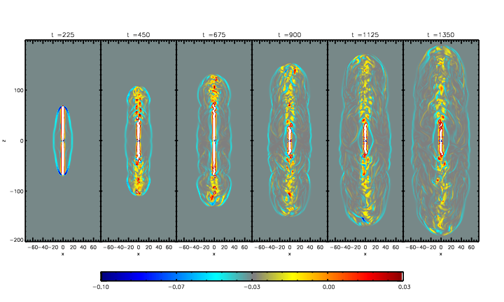
Figure 1: Snapshots of $j_{z}$ for the fiducial model showing the evolution of jet propagation and expansion. These snapshots are taken at the $y=0$ plane of a 3D simulation, at $t=225,450,675,900,1125,1350$, respectively. The spatial scales are normalized by $r_{\rm inj}$. Magnetic energy and flux are injected at the origin $x=y=z=0$ within $r=1$. The magnetic structure expands to form both a collimated jet along the $z-$axis that carries a strong (positive) outgoing current (indicated by the white-red-yellow color) and a “cocoon” enclosing the jet structure with the (negative) return current (blue color). The jet continues to propagate despite becoming unstable. With the instability, both the outgoing and return current paths show complicated structures, although the overall outgoing and return current patterns remain.

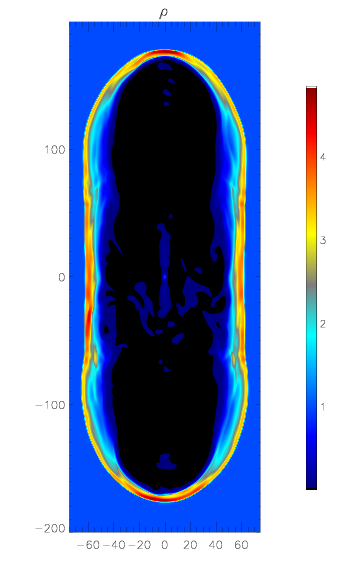
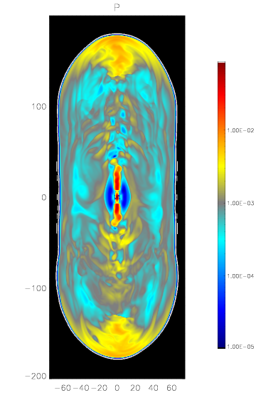
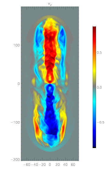
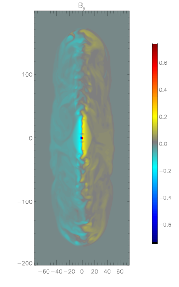
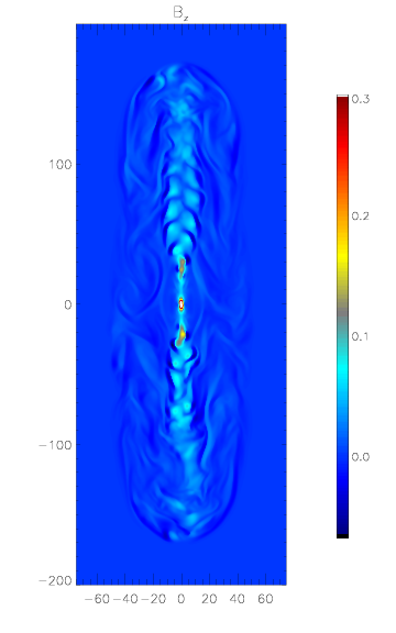
Figure 2: Snapshots of $\rho,P,v_{z},B_{y},B_{z}$ at a relatively late time $t=1125$ and at the $y=0$ plane for the fiducial run. The expansion is obviously much faster along the vertical direction than that in the transverse direction. A strong hydrodynamic shock is formed all around the (mildly) relativistically expanding outer boundary. The jet velocity is relativistic along the $z-$axis with $\gamma\sim$ a few but slows down significantly near the jet fronts. Magnetic fields fill up the volume enclosed by the swept-up hydrodynamic shell. The poloidal field dominates along the $z-$ axis but toroidal field dominates elsewhere.

Figures 1 and 2 show the overall morphology and evolution of the jet propagation. Over scales that are much larger than $r_{\rm inj}$, we find that the magnetic fields form an elongated structure that stays highly collimated, with the central axis (along $z$) having roughly a cylindrical shape without an obvious opening angle. While the central axis of the jet undergoes instabilities, the overall collimation and propagation still remain (to as long as we have simulated). The magnetic structure is enclosed by a hydrodynamic structure that consists mostly of a strong shock that is propagating into the background and sweeping up the material into a shell.

Figure 1 shows several snapshots of the z-component of current density $j_{z}$ at the $y=0$ plane. Because the injected fields possess a dipole-like poloidal field structure plus a toroidal field proportional to the flux function, the $j_{z}$ distribution has the overall structure that it contains an “outgoing” (positive) current along the central axis and a “return” current mostly in a thin shell encasing the structure. The location of the return current separates the magnetized interior from the non-magnetized outer region. Before $t\leq 225$, the jet appears to be propagating with little signature of nonlinear instabilities, while around $t\sim 300$, significant nonlinear instabilities first start to appear at the jet front, indicated by small wiggles with characteristic length scale $\sim$ a couple of tens $r_{\rm inj}$. At the late time many filamentary structures start to appear in jet front as the jet propagates further, while the central high $j_{z}$ region keeps almost the same vertical extent. It is interesting to note that the return current has maintained a quite axisymmetric cocoon-like shape throughout the duration of the run. At the late time, along the axis, the $j_{z}$ distribution splits into two parts: further away from the injection, the $j_{z}$ current density becomes highly unstable; whereas closer to the injection region with $|l_{z}|\leq 50~{}r_{\rm inj}$, it stays quasi-stable with relatively high peak current values (up to $j_{z,{\rm max}}=3.2$, not shown in the figure), presumably due to the strong injection.

To illustrate the jet properties at the late time, in Figure 2, we plot the snapshots of gas density $\rho$, gas pressure $P$, $z-$component of the gas three-velocity $v_{z}$, $y-$component of magnetic field $B_{y}$, and $z-$component of magnetic field $B_{z}$. In the density plot, there is a very thin layer of gas at the shock front with a maximum density $\rho_{\rm max}=4.8$, while inside this shell there is an extremely low density region with a minimum density $\rho_{\rm min}=7.9\times 10^{-4}$. This is a result of most of the uniform background gas being pushed away by the magnetic-dominated jet as it expands into the environment. Note in the inner $|l_{z}|\leq 40$ region there’s a small amount of gas which follows where the strong current is. This is because we inject a small amount of gas into the computational domain. At the end of this simulation, we have injected a total of $M_{\rm inj}=8688\rho_{0}r_{\rm inj}^{3}$, which for the parameters we specified at the end of §2, corresponds to a total mass injection of $1.3\times 10^{35}~{}{\rm g}$ and a mass injection rate of $0.09{\rm\,M_{\odot}}{\rm/yr}$. For the gas pressure, it is evident that the shock front has a higher pressure in the $z$ direction than in the horizontal direction, presumably due to the stronger expansion along the $z$ direction. For the gas velocity, we get the maximum Lorentz factor of the plasma flow is $\gamma_{\rm max}\sim 2.7$ and the maximum Lorentz factor generally increases with time during the run. For $v_{z}$, we see that while around the $r=0$ axis the gas is mostly moving outward, there’s also a returning component at larger $r$ due to the magnetic field structure we have used in our model. For the $B_{y}$ and $B_{z}$ plots, they show that, along the radial direction, the jet has a magnetic dominated core with $B_{z}$ being dominant at $r=0$ but $B_{y}$ becomes dominant at large $r$. Along the $z$ direction, there is a magnetic dominated region with $|l_{z}|\leq 50r_{\rm inj}$ that is followed by a more smoothly decreasing region out to the vertical extent of the jet. Overall, a magnetized central spine is always present.

To calculate the jet speed, we can follow the jet front and record its location as a function of time. Figure 3 shows how the location of jet front changes over time. Evidently, the jet front starts with an almost constant speed $\sim 0.3c$, and then its propagation speed changes at around $t\sim 300$, and gradually slows to $\sim 0.1c$. There is no slowing-down at the late time. Compared to the $j_{z}$ snapshots sequence in Figure 1, the turning point at the jet propagation occurs at the time when the nonlinear modes start to grow significantly.

3.1.2 Energy Transition

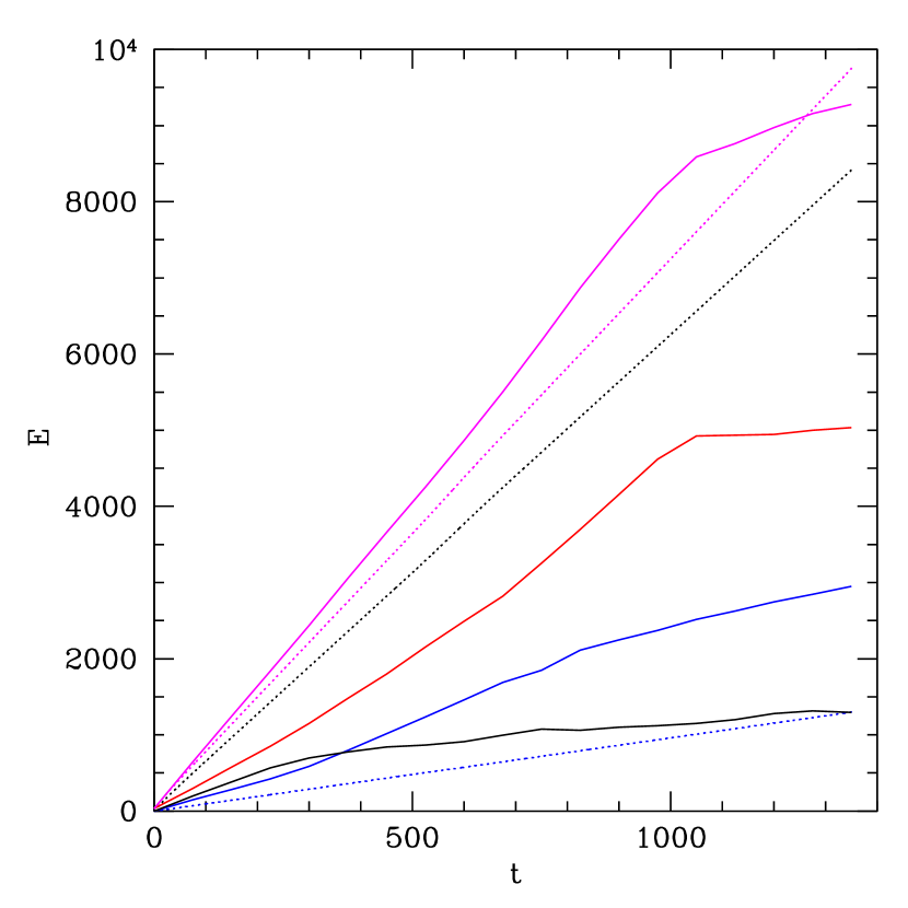
Figure 4: Evolution of different energy components of the fiducial run. Solid lines denote volume integrated energy and the dotted lines denote time and volume integrated injected energy. Black solid: $E_{\rm B}$; blue solid:$E_{\rm K}$; red solid: $E_{\rm U}$; magenta solid: $E_{\rm tot}$. Black dotted: $E_{\rm B,inj}$; blue dotted:$E_{\rm K,inj}+E_{\rm U,inj}$; magenta dotted: $E_{\rm tot,inj}+E_{\rm tot,0}$. The flattening at $t\sim 1000$ is due to energy flowing out of the computational domain. Even though the injected energy is predominantly magnetic, it gets converted into kinetic and thermal energies. So, the jet appears as having a large amount of kinetic and thermal energy. Note that the plotted quantities are volume integrated. In localized regions such as jet’s axis, magnetic energy can still be comparable to other energy components.

As the current-driven jet propagates further away from the injection region, instabilities grow and non-linear structures develop. These features also affect jet energetics, which is a central problem in jet physics. In Figure 4 we plot the evolution of volume-integrated total magnetic energy $E_{\rm B}$, total kinetic energy $E_{\rm K}$, total internal energy $E_{\rm U}$, and total energy $E_{\rm tot}=E_{\rm B}+E_{\rm K}+E_{\rm U}$. Note that magnetic energy density $e_{\rm B}$ includes all terms containing magnetic field, and it has a form of $e_{\rm B}={\mbox{\boldmath$B$}}^{2}/2+[|{\mbox{\boldmath$v$}}|^{2}|{\mbox{\boldmath$B$}}|^{2}-({\mbox{\boldmath$v$}}\cdot{\mbox{\boldmath$B$}})^{2}]/2$. For the kinetic energy density, we have excluded the rest mass energy, therefore $e_{\rm K}=(\gamma-1)\gamma\rho$. The internal energy density is $e_{\rm u}=p/(\Gamma-1)$. As a reference, we have also plotted the time and volume integrated injected magnetic energy $E_{\rm B,inj}$, injected kinetic energy $E_{\rm K,inj}$, and injected internal energy $E_{\rm U,inj}$. Note that for the injected energy the meaningful diagnostic here is to calculate the total injection up to a certain time $t$, $E_{\rm inj}(t)=\int_{0}^{t}\int\dot{E}_{\rm inj}dvdt$. It is obvious that although all energetics are increasing with the constant energy injection, after $t\sim 300$, $E_{\rm B}$ increases with a much shallower slope compared to the growth of $E_{\rm K}$ and $E_{\rm U}$. Before $t\sim 300$, the magnetic energy is larger than the kinetic energy but after that kinetic energy takes over.

We have also monitored the total energy conservation during the simulation. In Figure 4, the dotted magenta line represents $E^{{}^{\prime}}_{\rm tot,inj}=E_{\rm tot,inj}+E_{\rm tot,0}$, the total injected energy (magnetic + kinetic + thermal) plus the initial background energy, whereas the solid magenta line represents the sum of various energy components in the simulation domain. At the beginning they are quite close to each other, but as the simulation progresses, the difference between $E_{\rm tot}$ and $E^{{}^{\prime}}_{\rm tot,inj}$ continues to increase. The difference between these two total energies, however, is always much smaller than the other energy components in the simulation. This energy discrepancy is dominated by numerical errors and the origin of these errors in MHD simulations is relatively well known. For our simulations we have used both dual-energy formulation (evolving both internal energy and total energy equations) and energy fix after the constrained-transport to preserve the positivity of the thermal pressure. Both procedures break the total energy conservation in low pressure region and introduce energy error by a small amount. In addition, we find that these errors decrease gradually when we increase the numerical resolution. The sudden change in $E_{\rm tot}$ after $t\sim 1000$ is because the expansion has reached the computational domain boundaries and materials are flowing out of the box.

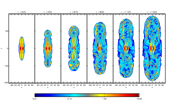
Figure 5: Snapshots of $\sigma$ for the fiducial model. Similar to Fig. 1, snapshots are taken from $t=225,450,675,900,1125,1350$, at $y=0$ plane. Large $\sigma$ indicates magnetic energy domination.

Our numerical model therefore gives an example of transferring jet’s magnetic energy into kinetic energy as jet propagates. The magnetization parameter $\sigma$, which we have chosen here as the ratio of Poynting energy flux to the kinetic energy flux, is $\sigma\equiv F_{\rm Poynting}/F_{\rm P}=B^{2}/4\pi\gamma^{2}\rho c^{2}$. In Figure 5 we plot several snapshots of $\sigma$ at the $y=0$ plane. As the jet propagates from its core region, the magnetically dominated region has been kept to be a region with a nearly constant extent $|l_{z}|\leq 50~{}r_{\rm inj}$. At late time, as the instability causes the jet fields to have more random and small structures, the jet can be seen in a more or less kinetically dominated state. Therefore, our numerical model illustrates a jet which contains a near-region with a $\sigma\gg 1$ and a far-region with a $\sigma\ll 1$. The jet does not stop nor get destroyed after this transition occurs. The energy transition is likely a result of current-driven instabilities.

3.1.3 Current-Driven Instabilities

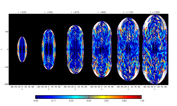
Figure 6: Snapshots of $q$ for the fiducial model. These snapshots are taken from $t=225,450,675,900,1125,1350$, at $y=0$ plane. $q<1$ denotes where the current is unstable to the kink mode.

In this section we give more details of the CDIs in the fiducial model. The primary candidate for CDIs is the kink instability. According to Kruskal-Shafranov criterion (Kadomtsev, 1966), a cylindrical MHD plasma with a constant current density $j_{z}$ in a confined radius is unstable to kink modes when $q=2\pi rB_{p}/(L_{z}B_{\phi})<q_{\rm crit}$, where $r$ is the cylindrical radius, $B_{p}$ is the poloidal component of the magnetic field which is parallel to the axis of the cylinder, $B_{\phi}$ is the toroidal field, and $L_{z}$ is the plasma column length. For ideal MHD, $q_{\rm crit}=1$, for RMHD, this number is a few (Narayan et al., 2009). This instability criterion indicates that when the jet is dominated by $B_{\phi}$, the jet will be unstable to the $m=1$ kink mode. This is indeed what we have observed in our simulations. In Figure 6 we have plotted $q$ at different times in the fiducial run, where we have chosen $L_{z}$ to be the height of the jet at the time. We can see that most of the near-axis and $|l_{z}|<50r_{\rm inj}$ region with large-current has $q<1$ throughout the simulation. Note that the Kruskal-Shafranov criterion is derived from the highly ideal situations and we should concentrate on the near-axis region where the large current is confined. The growth of CDIs is responsible for the slow-down of the jet front and facilitates the energy-transition process. For the physical parameters in our model, this growth period is $\gtrsim 100$ yrs.

One way to quantify the growth of the nonaxisymmetric modes is to calculate the power in the current using Fourier transform

$$f(m,k)=\frac{\int_{r_{\rm min}}^{r_{\rm max}}\int_{0}^{2\pi}\int_{z_{\rm min}}^{z_{\rm max}}|{\mbox{\boldmath$J$}}|e^{i(m\phi+kz)}rdrd\phi dz}{\int_{r_{\rm min}}^{r_{\rm max}}\int_{0}^{2\pi}\int_{z_{\rm min}}^{z_{\rm max}}rdrd\phi dz}$$ (15)

where $|{\mbox{\boldmath$J$}}|$ is the amplitude of the current density and the integration is over a cylindrical volume which encloses the current. In our calculation, we have used $r_{\rm min}=0$, $r_{\rm max}=10r_{\rm inj}$, $z_{\rm min}=0$, and $z_{\rm max}=200r_{\rm inj}$. $m$ is the azimuthal mode number and $k=2\pi/\lambda$ is the vertical wavenumber where $\lambda$ is a characteristic wavelength. The volume-averaged mode power in the current amplitude $|J|$ is then

$$P(m,k)=|f(m,k)|^{2}=\{{\rm Re}[f(m,k)]\}^{2}+\{{\rm Im}[f(m,k)]\}^{2},$$ (16)

where ${\rm Re}[f(m,k)]$ and ${\rm Im}[f(m,k)]$ are the cosine and sine Fourier transformations of $|{\mbox{\boldmath$J$}}|$, respectively.

In Figure 7 we plot the time evolution of $P(m,k)$ for the $m=0,1,2$ components for the fiducial run. For $k$, we have chosen $\lambda=20r_{\rm inj}$ for the characteristic wavelength (we have examined other wavenumbers and found they experience similar exponential growth). The $m=0$ component dominates throughout the run, although at late times the power in the nonaxisymmetric components has grown to be close to the power in the $m=0$ mode. The dominant nonaxisymmetric mode is the $m=1$ mode, and there is an exponential growth period between $t\sim 300-500$. After $t\sim 500$, the power in non-axisymmetric modes continues to grow, but at a rate which is much slower. There is also substantial power in the $m=2$ mode. Note that the background perturbations affect the onset time of significant growth: we have found that in another simulation with $50\%$ random background density perturbations, the onset time has changed significantly to about $t\sim 100$.

We have also observed magnetic Kelvin-Helmholtz instabilities due to the large shear that exists at various regions in the jet. The characteristic “cat eye” features can be observed at the jet front (e.g. see current near $z\sim 50r_{\rm inj}$ in $j_{z}$ slice at $t=450$ in Figure 1).

It is noteworthy that although instabilities occur in our models, the jet does not get totally disrupted and continues to propagate with an almost constant speed. This is partially due to the constant magnetic flux injection which continually drives the jet. The fact that the power in $m>0$ modes remaining smaller than the power in $m=0$ mode during the nonlinear stage is consistent with the non-disruption of the jet. We will discuss the possible explanation for stabilization in §4.

3.2 Effect of $\alpha$

The detailed properties of current-driven jets depend on the model parameters, one of which is the $\alpha$ parameter that represents the ratio of toroidal to poloidal fields. Effects of other parameters on the jet propagation will be examined in future studies.

In this simulation we use a higher $\alpha=40$, which gives a stronger toroidal field injection. In order to make comparison with the fiducial run, we try to keep the same magnetic energy injection rate, we have used a smaller magnetic field injection coefficient $B_{\rm inj,0}=0.054$. We found the jet propagates faster using this injection field configuration. We therefore have used a bigger vertical box extent of $L_{z}=800$ while keeping $L_{x}=L_{z}=150$ in order to accommodate the jet for the same run duration $t_{f}=1500$. We have also increased the grid size to $300\times 300\times 1600$ to keep the same resolution as that used in the fiducial run.

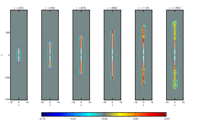
Figure 8: Similar to Fig. 1 but with snapshots of $j_{z}$ for the $\alpha=40$ model. These snapshots are taken from $t=225,450,675,900,1125,1350$, at the $y=0$ plane. The jet is much strongly collimated, presumably due to the stronger $B_{\phi}$ injections.

Figure 8 plots $y=0$ slices of the z component of current density $j_{z}$ at different times. Notice that the vertical size is twice as that in the fiducial run, then this jet definitely moves much faster than the fiducial jet. Compared to the $\alpha=10$ run, the non-linear features appear at a much later time, at a higher $z$ location, takes longer to grow, and the jet also has a leaner shape. In the $\alpha=10$ run, the non-axisymmetric modes appear to grow exponentially from $t\sim 300-500$, while here the instabilities do not start significant growth after $t\sim 500$. The current is also more concentrated toward the z-axis, most likely due to increased hoop pressure resulted from the larger $B_{\phi}$ component.

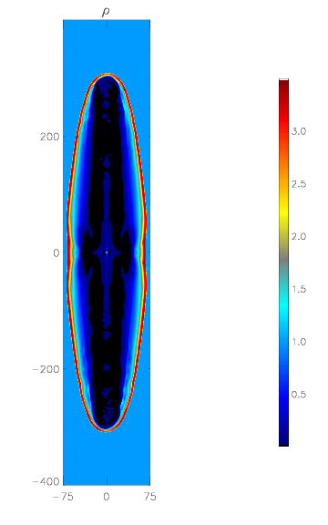
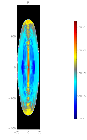
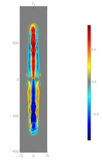
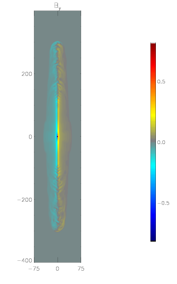
Figure 9: Similar to Fig. 2 but with snapshots of $\rho,P,v_{z},B_{y}$ at late time for the $\alpha=40$ run. These snapshots are taken from $t=1350$, at $y=0$ plane.

Figure 9 shows snapshots of $y=0$ plane cut-through for $\rho,P,v_{z},B_{y}$ at late time $t=1350$. Despite the more elongated jet shape, all the plotted quantities show qualitatively similar behaviors compared to the smaller $\alpha$ run. The Lorentz factor continues to increase over time and the highest Lorentz factor achieved in this run is about $\gamma\sim 2.4$. We suspect this number will increase more as the jet has not developed much non-linear features at the end of run. However, it is not clear what determines the terminal $\gamma$ in our models, as it needs a much bigger computational domain size as well as longer simulation run time.

Figure 10 illustrates the propagation of jet front for $\alpha=40$ case. The slowing down of jet front does not occur until $t\sim 1200-1300$, much later compared to the smaller alpha case. Although the injected magnetic energy rate is the same, the jet propagates with a larger bulk velocity because the dominant toroidal components, consistent with predictions by the magnetic tower models (see discussion in the §4).

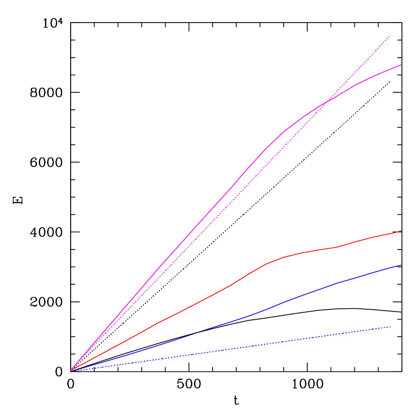
Figure 11: Energetics of the $\alpha=40$ run. Color scheme is the same as in Figure 4.

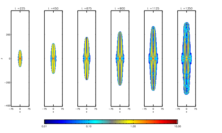
Figure 12: Snapshots of $\sigma$ for the $\alpha=40$ model. These snapshots are taken from $t=225,450,675,900,1125,1350$, at $y=0$ plane.

We have observed similar behavior for total energetics in this model as in the $\alpha=10$ case, as shown in Figure 11. Similar to the fiducial run, the total kinetic energy takes over the magnetic energy after the instabilities grow, and both the kinetic energy and internal energy increase with the continuous conversion of magnetic energy into these two energies. $E_{\rm K}>E_{\rm B}$ occurs at a later time compared to the fiducial run, consistent with the onset of non-linear features. At the end of the simulation, the total $E_{\rm K}$ is quite similar to the $E_{\rm K}$ in the fiducial run, $E_{\rm B}$ is $\sim 34\%$ larger than that in the fiducial run, and the total internal energy is $\sim 27\%$ smaller than in the fiducial run. This smaller dissipation is also consistent with the later onset of non-linear features. The smaller energy transition can also be seen from the magnetization parameter $\sigma$ images. Figure 12 shows $\sigma$ at $y=0$ slices at different times for this run. It is clear that, when compared to the fiducial run, the energy transition occurs mainly at a later time too, consistent with the onset time for the significant non-linear interactions. This means for the same amount of total magnetic energy injection, when $\alpha$ is larger, the energy transition will occur further away from the jet launching location.

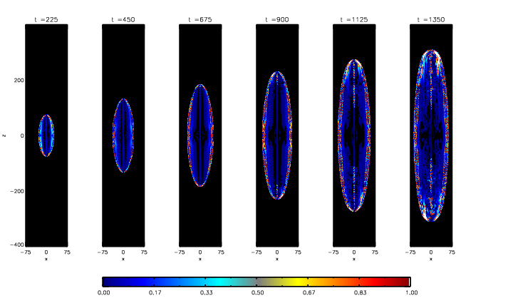
Figure 13: Snapshots of $q$ for the $\alpha=40$ model. These snapshots are taken from $t=225,450,675,900,1125,1350$, at $y=0$ plane. $q<1$ denotes when the current is unstable to the kink mode.

How about CDIs? Figure 13 plots the snapshots of value of $q$ for the kink instability limits at $y=0$ slices. For a certain cylindrical current, when $\alpha$ increases, the $q$ value decreases for the same cylindrical shape. Therefore, the jet will still be unstable due to the kink instabilities, and this is what we have observed here.

To see the detailed interplay between axisymmetric and non-axisymmetric modes, we have calculated the power of first few modes in this model. Figure 14 shows the growth of mode power of the amplitude of current for this run. Similar to the lower $\alpha$ model, the dominant non-axisymmetric mode is the $m=1$ kink mode. Throughout the simulation the axisymmetric $m=0$ mode dominates, although the $m=1$ mode almost grows to a similar magnitude at the late time, which introduces the non-linear behaviors. However, the growth rates of non-axisymmetric modes are smaller compared to the smaller $\alpha$ case. This is somewhat surprising as the larger $\alpha$ is expected to lead to a stronger instability. One possible explanation is that, while the linear analysis for the growth rate of kink instability is based on the ideal setup of a constant cylindrical current with well-defined geometry and fixed boundaries, here we are dealing with an evolving jet with continuous magnetic injection at the center and the jet itself is fast propagating in the vertical direction and expanding in the transverse directions. Therefore instability analysis from ideal plasma physics derivation may not be applied directly to our evolving system. Further discussions on this result are given in §4.

To understand the dependence of the CDI’s on-set on injection parameters, we also make a run where the poloidal field injection rate is the same as the fiducial run ($B_{\rm inj,0}=0.2$) while keeping $\alpha=40$ (hence a higher total magnetic energy injection rate), we find that instabilities grow at a rate that is more close to that in the fiducial run, and the jet front propagation speed turn-over occurs earlier, at $t\sim 400$ (see the dashed line in Figure 10). This indicates that the growth of CDIs and the onset of nonlinear features in these propagating current jet systems are a complex process probably depending more on the parameters for the magnetic field injection profile (both magnitude and shape), and we will explore this more in the future.

3.3 Effect of a Disk

Our simulations show that the magnetic structure expands both along the $z-$axis and sideways. As the jet is a consequence of accretion, and in the spatial scales we are considering, the accretion disk should surround and extend into the injection region. In this section, we use a toy model to investigate the effect of possible disk confinement and whether the instabilities will still occur when there is a gas-pressure-supported disk at the jet base. All the jet parameters are the same as in the fiducial run.

The reason to choose a gas pressure-supported disk instead of a rotation-supported disk is mainly of numerical consideration. For a more physical accretion disk with rotation, the simulation requires a much smaller time step, in order to resolve the disk rotation. We therefore choose a gas pressure supported disk which is initially in a hydrostatic equilibrium, and this is numerically much easier than evolving a rotating disk. We are not modeling the accretion process itself, but focusing on how the gas pressure will confine the jet shape and whether the disk will affect the instabilities.

We have solved the effective gravitational potential $\Phi_{\rm eff}$ which is able to hold a gas disk with a density distribution

$$\rho(r,z)=\rho_{\rm bkg}+\frac{\rho_{0}}{(1+r/r_{0})^{3/2}}\exp{(-\frac{z^{2}}{2H^{2}})},$$ (17)

where the disk is centered at $x=y=z=0$, $r=(x^{2}+y^{2})^{1/2}$, $\rho_{0}$ is the characteristic disk midplane (defined as $z=0$) gas density, $r_{0}$ is a characteristic disk radius, and $H$ is the disk scale height. When choosing $\rho_{0}\gg\rho_{\rm bkg}$, the first term in the density equation can be omitted. $\Phi_{\rm eff}(r,z)$ can be solved by considering the Euler equation in the radial and vertical directions. Because there is no rotation and we seek steady-state solutions, the equations are a set of partial differential equations (PDE) of a simple form:

$$\begin{matrix}\partial_{r}\Phi_{\rm eff}(r,z)=-\frac{1}{\rho(r,z)}\partial_{r}p,\\ \partial_{z}\Phi_{\rm eff}(r,z)=-\frac{1}{\rho(r,z)}\partial_{z}p.\end{matrix}$$ (18)

Assuming a simple, constant sound speed $c_{s0}$, the solution of the above PDE can be obtained by integrating separately along $r$ and $z$ directions. $\Phi_{\rm eff}(r,z)$ has a form

$$\Phi_{\rm eff}(r,z)=c_{s0}^{2}[\ln(1+(\frac{r}{r_{0}})^{3/2})+\frac{z^{2}}{2H^{2}}].$$ (19)

For simplicity we have omitted the constant term. Including a non-trivial $\rho_{\rm bkg}$ term in the disk density distribution makes solving $\Phi_{\rm eff}(r,z)$ much more complex.

To set up this disk, we have chosen $\rho_{0}=100$ which is much greater than the background density in the whole simulation box. We choose $r_{0}=10r_{\rm inj}$, $H=r_{\rm inj}$, and the same sound speed used for the background gas. The inner edge of the disk is set at $r_{\rm inj}$ and outer edge of the disk extends to the edge of the box. The disk is thin in most of the regions except in the inner few $r_{\rm inj}$. We have tested our effective gravitational potential $\Phi_{\rm eff}(r,z)$ and the associated disk density distribution $\rho(r,z)$. In the case of zero injection, our disk can indeed be held in a hydrostatic equilibrium by the effective potential. After injecting the strong magnetic flux into the center region, the disk cannot be retained in its original equilibrium, and will be pushed outward by the strong magnetic pressure. Again, our emphasis of this toy model is to test whether the inclusion of a gaseous disk will change the properties of the propagating jet, especially the path of the return current profile.

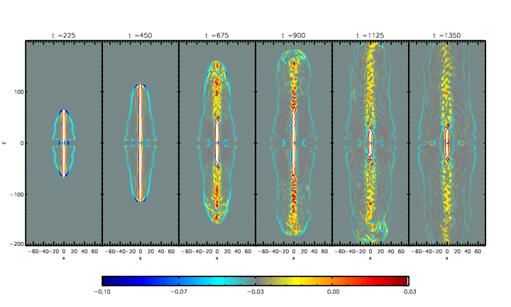
Figure 15: Snapshots of $j_{z}$ for the disk model. These snapshots are taken from $t=225,450,675,900,1125,1350$, at $y=0$ plane.

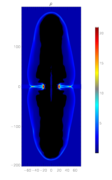
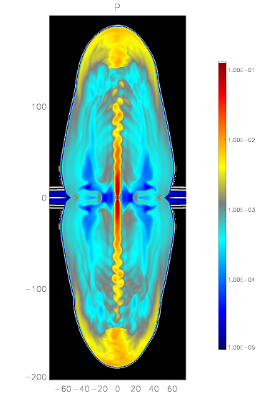
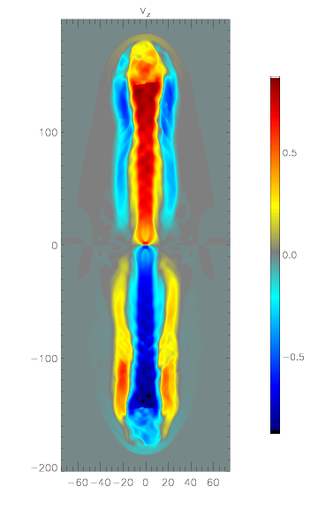
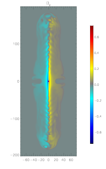
Figure 16: Snapshots of $\rho,P,v_{z},B_{y}$ at late time for the disk run. These snapshots are taken from $t=900$, at $y=0$ plane.

Figure 15 shows the current density slices at different times when including this gas disk. Compared to the fiducial run, near the base of the jet ($z\leq 10r_{\rm inj}$), the jet expands less in the equatorial plane. The return current is also much closer to the axis in this region (which changes the magnetic field shape more paraboloidal). The overall shape of the jet resembles more of an observed astrophysical jet in this situation, with an opening angle at its base due to the disk confinement. Other quantities are shown in Figure 16, which gives snapshots of $\rho,P,v_{z},B_{y}$ at the late time. The disk component can be clearly seen in these snapshots. The magnetic pressure is gradually pushing the disk outward due to the constant flux injection, even at the late stage of the simulation: our disk never reaches a static state in this model and this is due to the fact that we are not simulating a real accretion event here. However, our simple toy model provides a glimpse into what a more realistic disk-jet simulation would illustrate in the future.

More importantly, on the larger vertical distance, the jet displays a very similar morphology as in the fiducial run. The jet is well collimated, the CDI grows and non-linear features have developed as jet propagates beyond a few tens of $r_{\rm inj}$. In Figure 17 we have plotted the propagation of jet front. It is obvious that jet front has already reached the vertical edge of the box at $t=1000$. The jet front propagates with a high speed for a longer duration ($t\sim 450$) than in the fiducial case. After this stage the jet front propagation slows down but is still slightly faster than in the fiducial case, most likely due to the extra ”pinch” effect at its base.

For instabilities, from instability criterion and mode power analysis we find their general properties are quite similar to the fiducial run, although the instability growth rate is slightly larger. This is not surprising because the instabilities are driven by the injected current, and how they grow is a reflection of the intrinsic property of the jet current at large distance, rather that the environment confinement provided at its base.

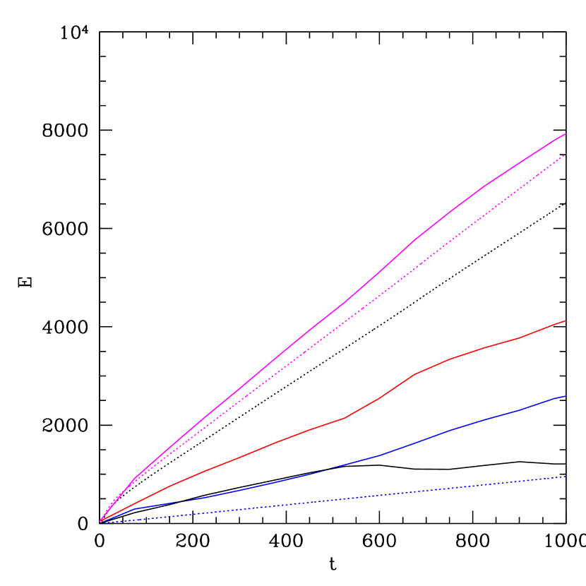
Figure 18: Energetics of the disk run. Color scheme is the same as in Figure 4.

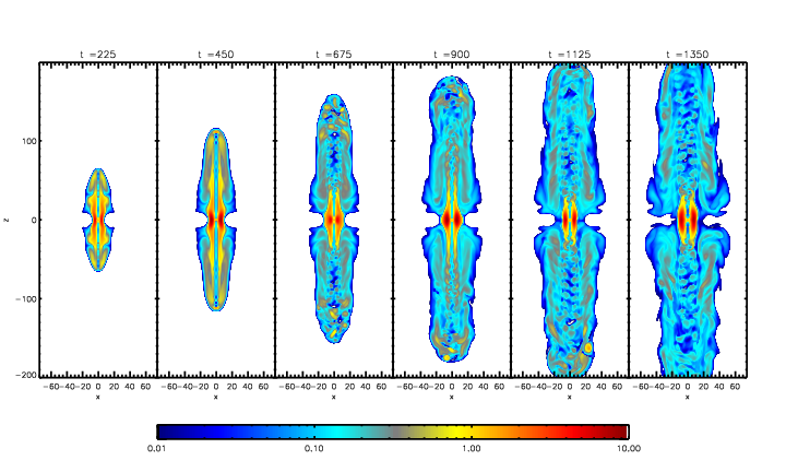
Figure 19: Snapshots of $\sigma$ for the disk model. These are taken from $t=225,450,675,900,1125,1350$, at $y=0$ plane.

For energy transition, Figure 19 shows $\sigma$ at different time. This illustrates that, even with a disk, at distances far from the disk and injection region, the instabilities introduce large dissipation and magnetic energy is transformed into kinetic and thermal energies. We have also calculated the evolution of energetics of the total box, as shown in Figure 18. We get quite similar results compared to the fiducial run: total kinetic energy takes over the magnetic energy after the instabilities grow, and both the total kinetic energy and the total internal energy increase as magnetic energy is converted into these two energies over time.

We have made additional runs by changing the disk scale height $H$ to a different value ($H=5r_{\rm inj}$ which sets up a thicker disk), similar results were obtained.

3.4 Resolution Study

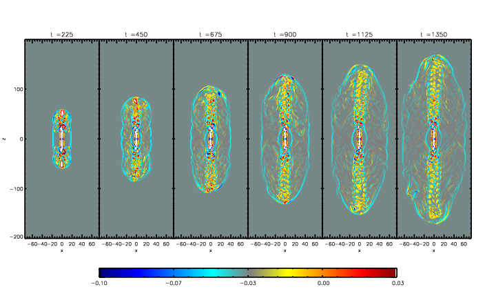
Figure 20: Snapshots of $j_{z}$ for the fiducial model with higher resolutions. Snapshots are taken from $t=225,450,675,900,1125,1350$ at $y=0$ plane.

In order to illustrate the effects of resolution, we have re-run the fiducial case with a higher resolution $N_{x}=N_{y}=450,N_{z}=1200$, while keeping all other parameters unchanged. Figure 20 shows the $j_{z}$ current density slices at the $y=0$ plane. Compared to the fiducial run, the non-linear features appear earlier, already apparent at $t\sim 200$. At the late time, the jet has a more pronounced “spine”, where large scale wiggles in this spine are visible near both sides of the jet front. The return current also exhibits asymmetric morphology, and extends slightly further away from the axis in the equatorial plane. Recently, Mignone et al. (2010) have studied resolution effects in RMHD simulations of jets. They also observed that as jet propagates further its trajectory becomes more curved, moving from the central axis. This effect is more pronounced in their higher resolution runs. We note our findings are consistent with their results.

Comparing the jet front location at different times for both runs, we find that the higher resolution jet propagates first with a similar speed compare to that in the fiducial run. Its slowing-down point, however, occurs earlier at $t\sim 150$ due to the early onset of the non-linear stage. After $t\sim 150$, the jet propagates again with the similar speed as in the fiducial run. This explains why the jet front reaches a lower $z$ height compared to the fiducial run at the late time.

Although the resolution does not affect much of the overall jet dynamics, it certainly affects the instabilities. From the mode analysis we find that the higher resolution simulation also gives an almost doubled growth rate for non-axisymetric modes, which causes the current profile to become nonlinear at $t\leq 200$.

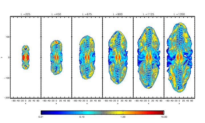
Figure 21: Snapshots of magnetization parameter $\sigma$ for the fiducial model with higher resolutions. These snapshots are taken from $t=225,450,675,900,1125,1350$, at $y=0$ plane.

Also similar to Mignone et al. (2010), we find more and stronger shocks in the high resolution run. This introduces more dissipation and gives a larger total thermal energy. As a result, we also notice that both the total kinetic energy $E_{\rm K}$ and the total magnetic energy $E_{\rm B}$ are smaller in the higher resolution run: for example, $E_{\rm B}$ is $\sim 11\%$ smaller than that in the fiducial run and $E_{\rm K}$ is $\sim 7.6\%$ smaller at $t\sim 600$ when both models are at the non-linear stage. The magnetic-to-kinetic energy transition still occurs in the higher resolution run. We have plotted $\sigma$ parameter at $y=0$ plane at different times for this model, as shown in Figure 21. We can see that at the “spine” region of the jet $\sigma$ is smaller, indicating higher resolution leading to a more efficient energy transition.

Lastly, we want to stress that although our higher resolution simulation has displayed quantitatively similar behaviors as those in the fiducial run, such as the development of CDIs and the energy transition, our numerical model of RMHD jet has not shown signs of convergence. The convergence issue is therefore out of the scope of this paper, and needs further investigation.

4 Summary and Discussion

We have carried out new RMHD simulations for Poynting-flux driven jets in AGN systems. The computational domain is relatively large so that both the injected magnetic fluxes and their subsequent evolution are contained well within the simulation domain. The fluxes which are responsible for driving the jet are injected at the center of the box, with an injection region size $r_{\rm inj}$. The flux injection rate is continuous and is taken to be constant. Our injected magnetic fields have an axisymmetric geometry with close field lines, consisting of a poloidal field plus a dominant toroidal field component. We follow the propagation of the jet to a few hundreds of $r_{\rm inj}$ in three dimensions. We proposed to scale the injection region $r_{\rm inj}$ to $\sim 10^{3}$ gravitational radii of a black hole, thus our simulations could be relevant to observations of AGN jets on from sub-pc to tens of pc scales.

We find these jets are well-collimated. They have a concentrated “spine” that is roughly of the same size of the injection region inside which the majority of the out-going current is flowing, along with a significant fraction of the injected poloidal flux. Driven by the strong magnetic pressure gradient in the $z-$direction, it eventually develops relativistic speeds. The magnetic structure also expands transversely, though at a much reduced speed. This sideway expansion is limited by the inertia of the swept-up background material.

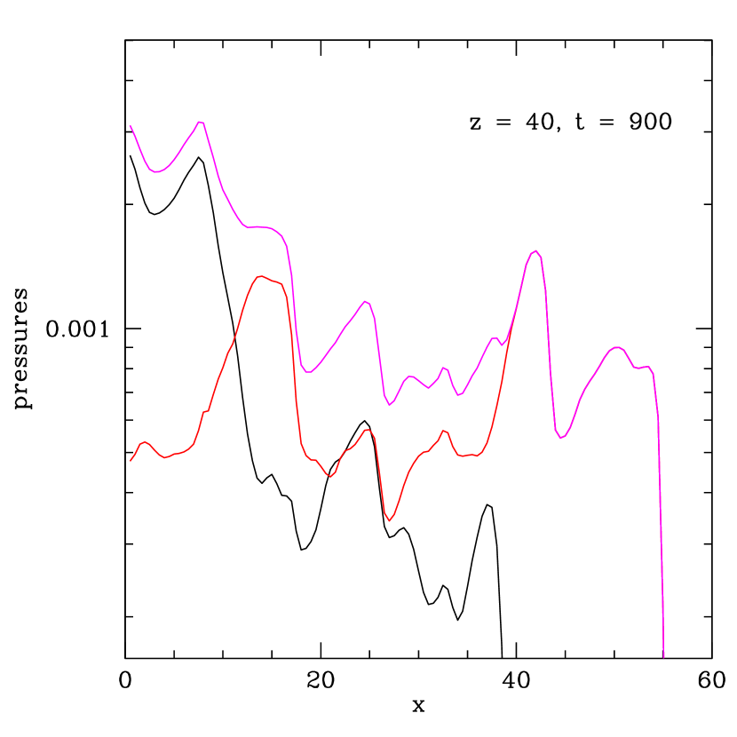
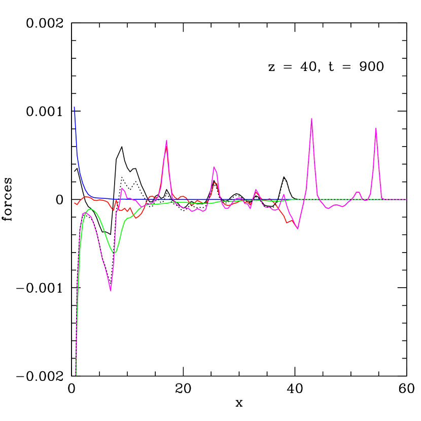
Figure 22: Radial profiles of physical quantities along the x-axis in the equatorial plane with $(y,z)=(0,40)$ at $t=900$ in the fiducial run. Left: pressures in the radial direction. Black: magnetic pressure $p_{\rm m}$; red: gas pressure $p$; magenta: total pressure $p+p_{\rm m}$. Right: forces in the radial direction. Black solid: magnetic pressure gradient $F_{\rm mp}$; red: gas pressure gradient $F_{\rm p}$ ; blue: centrifugal force $F_{\rm c}$; green: magnetic tension force $F_{\rm t}$; black dotted: sum of magnetic pressure gradient and tension force $F_{\rm\bf J\times B}=F_{\rm mp}+F_{\rm t}$; magenta: total of magnetic forces and gas pressure gradient $F_{\rm total}=F_{\rm\bf J\times B}+F_{\rm p}$.

To understand better why the magnetic structure is highly collimated along the central axis, we consider the force balance in the radial direction for the fiducial model, at $t=900$, and vertical height $z=40r_{\rm inj}$, as shown in Figure 22. We choose $z=40r_{\rm inj}$ because at this height the jet is still quite axisymmetric, has propagated far enough in the vertical direction, and non-linear features from instabilities are not severe. At this height, the magnetically dominated part of the jet extends from $x=0$ to $\sim 10r_{\rm inj}$, with the return current located at $x\sim 40r_{\rm inn}$. The outer edge of the hydrodynamic shock is located at $x\sim 55r_{\rm inj}$. The left panel of Figure 22 shows that inside $x\sim 10r_{\rm inj}$, magnetic pressure $p_{\rm m}$ dominates over gas pressure $p$ $(\beta\ll 1)$ while both keep a relative flat distribution along the radial direction; outside $x\sim 10r_{\rm inj}$, magnetic pressure starts to drop quickly while gas pressure continues to rise until $x\sim 15r_{\rm inj}$. We can compare this result to the analysis of non-relativistic MHD simulation of Nakamura et al. (2006) (their Figure 10). At large radial distances, $x\sim 55r_{\rm inj}$, since the plasma pressure is much larger than the background pressure $\sim 10^{-4}$, the radial expansion of the jet structure is limited by plasma inertial.

The right panel shows the various forces in the radial direction: near the inner jet edge, in the $10r_{\rm inj}\leq x\leq 15r_{\rm inj}$ region, the dominant force is the outward magnetic pressure gradient $F_{\rm mp}=-\partial_{r}(B_{\phi}^{2}+B_{z}^{2})$, and there is also a smaller inward magnetic tension force $F_{\rm t}=-B_{\phi}^{2}/r$. The sum of the two, the total Lorentz force $F_{\rm\bf J\times B}$ is slightly larger than the inward gas pressure gradient $F_{\rm p}=-\partial_{r}p$, although the magnitudes of the two are comparable. Inside $x\sim 10r_{\rm inj}$, the largest force is the inward magnetic tension force $F_{\rm t}$ provided by the strong toroidal field, which gives a pinch effect. This effect is largely consistent with the effects of magnet hoop stress in the “magnetic tower” models (Lynden-Bell, 1996, 2003; Li et al., 2001). There is a small rotation of gas that has also been produced near the axis as seen by a non-trivial outward centrifugal force $F_{\rm c}=\gamma\rho v_{\phi}^{2}/r$. Further out from the jet axis, all the magnetic forces varnish and we can see a few hydrodynamic shock wave fronts. It is also worth pointing out that although our jet is magnetically dominated (see the magenta curve, sum of gas pressure gradient and Lorentz force $F_{\rm total}$), it is not exactly force-free, as ${\bf J\times B}$ is not exactly zero inside the jet (black dotted curve). Furthermore, the non-zero total force also implies that the jet is not in a force balance.

The jets we have obtained in these simulations are mildly relativistic, with the largest Lorentz number about $\gamma\sim 3$ (although the jet front is slowed down by the shocks), while the small amount of injected mass has an injection velocity of $v_{\rm inj}=0.5c$ initially. Acceleration is therefore achieved through magnetic processes and we have observed $\gamma_{\rm max}$ increases with time with no signs of slowing-down. Due to the limit of the computational resources, we have not yet been able to determine the terminal speed of the jet in our models. However, it is plausible that a higher flux injection rate and/or a higher $\alpha$ can lead to a higher speed. Another issue is purely numerical: in RMHD/GRMHD simulations there is a small amount of mass loading, and the choice of density floor probably affects strongly $\gamma_{\rm max}$ (e.g. McKinney & Gammie (2004)). In our simulations we have also injected a small amount of gas in the injection region (see discussion below), which helps us to maintain the validity of the RMHD integration scheme, especially in the injection region where the magnetic field is the strongest.

These jets also display current-driven instabilities and undergo subsequent strong dissipations. However, the jets are not disrupted and are able to propagate to large distances in our simulations. The cylindrical jet current is unstable most to the $m=1$ kink mode, which undergoes an initial period of exponential growth. Depending on the model parameters, outside a few tens to hundreds of $r_{\rm inj}$, the mode growth slows down and the non-linear interaction among the modes leads to apparent non-linear features such as filaments in the current and occasional large scale “wiggles” in the jet spine. Large amounts of dissipation are also introduced outside this region. As a consequence, as the jet propagates further away from its launching location, much of magnetic energy has been transformed into jet kinetic energy and heat, although the jet is still collimated and continues to propagate, albeit at a slower speed. We notice that although the $m=1$ mode grows exponentially, its power remains smaller than the power in the $m=0$ mode throughout the simulations. This is consistent with the fact that the jet is not disrupted even with CDI present. Such non-disruption behavior of jet is consistent with the past RMHD simulations. These results also support the idea some other mechanisms may be at work to suppress the non-linear impact of CDIs (e.g., Narayan et al. (2009)).

We suggest that the ability of jets to avoid the complete disruption is due to both the rapid jet propagation and the fast evolution of the associated underlying magnetic structure, which we collectively term “dynamic stabilization”. Away from the injection region, the Alfvén speed in the magnetized region decreases from $\sim 0.9c$ near the central spine to $\sim 0.2-0.6c$ near the boundaries. The background flow (except that near the jet front), however, still has a relativistic speed of $>0.9c$. It is therefore possible that this fast background flow has modified the physical quantities faster than the instability growth timescale. The same arguments can be applied to the large $\alpha$ runs when the magnetic structure tends to evolve even faster. In other words, the CDIs developed in our simulated jets are quite convective, rather than being absolute instability. To the extent we can simulate the jet propagation, it remains collimated and propagating at a steady speed. It therefore remains to be seen how dynamical stabilization will continue to help jets survive the instabilities and whether the environmental factors may play some additional roles in determining the fate of relativistic jets.

We have also shown that as these current-carrying jets propagate far from the injection region, magnetic energy can be transformed into kinetic energy of the jet and also generates heat. The magnetization parameter $\sigma$, although much larger than one at the jet base, can become much smaller with $\sigma\ll 1$ in the region where CDIs have grown to display non-linear features. Note that in our model the smaller $\sigma$ is not a result of the jet shocking on the external medium, but a consequence of development of CDIs in a current-carrying jet. Although many non-linear features of CDIs appear in our models, the model has not reached a saturated state: all the energetics in the models still increase over time and it is not clear what the jet dynamics will be on an even longer time scale. Future simulations of larger computational domain with longer evolution time are needed to give a more comprehensive picture of the $\sigma$ question. Recent local simulations of CDIs by O’Neill et al. (2012) have also shown that development of CDIs are able to convert magnetic energy into kinetic energy and thermal energy, and they also have not found a saturated state. Nevertheless, all these simulations are starting to show that CDIs are indeed able to tackle the $\sigma$ problem.

In our high resolution run we have observed some large scale wiggles near the jet fronts. In the future it would be interesting to see whether these models are able to produce knots and spots along the jet axis, which are often observed in AGN jets. All our models also produce a central current (“spine”) along the vertical axis, and a cocoon-like return current which locates at a large distance from the jet axis and encloses the central jet. In the high resolution run this return current also exhibits non-axisymmetric features. These return currents have also been produced in the past MHD simulations (e.g. Ustyugova et al. (2006); Li et al. (2006); Nakamura et al. (2006, 2007, 2008)). It would be interesting to see whether these large scale return currents are observable (e.g. Kronberg et al. (2011)). Time-dependent jet properties produced in this work, when combined with radiative processes, can also be used to compare with observational features of AGN jets, such as their time variability. This work marks our first effort toward producing AGN jet diagnostics from a numerical RMHD model.

It would be useful to scale the model parameters for a supermassive black hole system. As discussed in §2, for a $3\times 10^{9}{\rm\,M_{\odot}}$ black hole as the one at the center of M87, we have a magnetic energy injection rate of $5.2\times 10^{46}{\rm\,ergs^{-1}}$ (the Eddington luminosity is $L_{\rm Edd}\sim 3.9\times 10^{47}{\rm\,ergs^{-1}}$). This current-carrying jet can propagate from its injection region of size $r_{\rm inj}\sim 0.14{\rm\,pc}$ to a distance of $\sim 28{\rm\,pc}$ in the fiducial model, and to a distance of $\sim 56$ pc in the $\alpha=40$ model, without being disrupted. The features of CDIs show up on the pc scales. The magnetic field has a strength that is on the order of $10^{-3}{\rm G}$ in the jet axis and far from the core. The total current is estimated to be $I\sim 10^{18}{\rm amp}$ in the fiducial model. For the background gas, we have adopted a uniform background density of $10^{2}{\rm cm}^{-3}$ and temperature of $5{\rm keV}$. We will explore the effect of background profile in the future investigation. We have also injected a small amount of gas in the injection region, and in the fiducial model the mass injection rate is $\dot{M}_{\rm inj}\sim 0.09{\rm\,M_{\odot}}{\rm yr^{-1}}$, which is much smaller than the Eddington accretion rate $\dot{M}_{\rm Edd}\sim 13{\rm\,M_{\odot}}{\rm yr^{-1}}$. (Usually we need to inject more mass if the magnetic energy injection rate is increased due to numerical reasons.) Lastly, for the resolution, in the fiducial model the smallest length scale is $\Delta l\sim 0.01{\rm\,pc}$ and the smallest time scale is $\Delta t\sim 20$ days. Note this time scale is still long compared to the time scale on which the TeV flares operate. Therefore, pushing to higher resolution deserves more efforts in future studies.

We have investigated the fiducial model with two different resolutions, and both exhibit qualitatively similar behaviors. However, the convergence is not achieved: this is especially true for the instability and the shocks; effect of resolution on energy transition is not clear yet. We will leave the even higher resolution studies to the future work. We have also investigated a model with a higher toroidal-to-poloidal injection ratio. The details of the injection function definitely affect jet properties. In the future, we will explore more model parameters including magnetic field geometries, injection functions, and external environment profiles (e.g. power-law external pressure profiles used in Komissarov et al. (2009)).

We have chosen an injection model that has closed poloidal field lines, which causes $B_{z}$ change directions beyond $r_{\rm inj}$ with no net-flux. Different field injection configuration exists. For example, past GRMHD black hole accretion simulations have explored models with initial configurations with open field lines/net flux (e.g. ”Magnetically Arrested Disc” models). However, whether the disk has net-flux or not is a un-resolved question, largely owing to our lack of knowledge of disk dynamo. Since these past simulations have not typically produced the jet structure at large scales where comparison with observations becomes more feasible, it is therefore of interest to explore the case with zero net-flux. Furthermore, studies of large-scale jets in the intra-cluster medium (hereafter ICM; Li et al. (2006); Nakamura et al. (2006, 2007, 2008)) have argued that magnetic tower model provides good fits to observations of jet s morphologies in the ICM. Future work is therefore needed to explore different initial field configurations and their consequences in jet stability and dissipation.

Lastly, we want to point out that recently there has been great progress in the laboratory experiments to study current-driven instabilities in jets (e.g. Hsu & Bellan (2005); Bergerson et al. (2006)). Although the physical conditions in our AGN jet models differ greatly from the parameters in laboratory jets (e.g. density, current etc.), it would be of great interest to see whether laboratory plasma experiments can teach us the general principles in understanding astrophysical jets.

Table 1: Units of Physical Quantities For Normalization

Physical Quantities	Description	Normalization Units	Typical Values
$r$ $[=(x^{2}+y^{2}+z^{2})^{1/2}]$	Length	$r_{\rm inj}$	0.143pc
$v$	Velocity field	c	$3.0\times 10^{10}{\rm\,cm\,s^{-1}}$
$t$	Time	$r_{\rm inj}/c$	0.47yr
$\rho$	Density	$\rho_{0}$	$1.67\times 10^{-22}{\rm\,g\,cm^{-3}}$
$P$	Pressure	$\rho_{0}c^{2}$	$0.15{\rm dyncm}^{-2}$
$B$	Magnetic field	$(4\pi\rho_{0}c^{2})^{1/2}$	$1.38{\rm G}$
$E$	Energy	$B^{2}r_{\rm inj}^{3}/(8\pi)$	$6.52\times 10^{51}{\rm\,erg}$
$P$	Power	$B^{2}r_{\rm inj}^{2}c/(8\pi)$	$4.42\times 10^{44}{\rm\,ergs^{-1}}$

Figure 3: The location of jet front along the $z-$ direction as a function of time in the fiducial run. The time when the jet slows down ($t\sim 300$) is consistent with the appearance of instabilities as shown in Fig. 1.

Figure 7: Evolution of various mode power in the current distribution for the fiducial run. Solid lines: $m=0$; dotted lines: $m=1$; dashed lines: $m=2$. The axisymmetric component remains dominant throughout the jet evolution. The non-axisymmetric modes show exponential growth but relatively low saturation level at the nonlinear stage.

Figure 10: The location of jet front as a function of time in the $\alpha=40$ runs. Jet slows down after the non-axisymmetric modes become significant compared to the axisymmetric mode. Solid: $\alpha=40$ with the same total magnetic energy injection rate as the fiducial run; dotted: $\alpha=10$ fiducial run; dashed: $\alpha=40$ but with a larger magnetic energy injection rate.

Figure 14: Evolution of mode power in the current for the $\alpha=40$ run. Solid lines: $m=0$; dotted lines: $m=1$; dashed lines: $m=2$.

Figure 17: The location of jet front as a function of time in the disk run (solid line). Jet slows down after the nonlinear modes start to grow. Dash line: jet front locations in the fiducial run.

.

References

- Aharonian et al. (2007) Aharonian F. et al., 2007, ApJ, 664, L71
- Albert et al. (2007) Albert, J. et al., 2007, ApJ, 662, 892
- Baty & Keppens (2002) Baty, H., & Keppens, R., 2002, ApJ, 580, 800
- Bergerson et al. (2006) Bergerson, W. F., Forest, C. B., Fiksel, D. A., Hannum, R., Kendrick, J. S., Stambler, S., 2006, Phys. Rev. Lett.96, 015004
- Biretta et al. (1991) Biretta, J. A., Stern, C. P., & Harris, D. E., 1991, ApJ, 101, 1632
- Beckwith et al. (2008) Beckwith, K., Hawley, J.F., Krolik, J.H., 2008, ApJ, 678, 1180
- Begelman (1998) Begelman, M.C., 1998, ApJ, 493,291
- Blandford & Znajek (1977) Blandford, R.D. & Znajek, R. L., 1977, MNRAS, 179,433
- Colella & Woodward (1984) Colella, P. & Woodward, P.R. 1984, JCoPh, 54, 174
- De Villiers et al. (2003) De Villiers, J. -P., Hawley, J. F., & Krolik, J. H., 2003, ApJ, 599, 1238
- De Villiers et al. (2005) De Villiers, J. -P., Hawley, J. F., Krolik, J. H. , & Hirose, S. 2005, ApJ, 620, 878
- Hardee (2007) Hardee, P. E., 2007, ApJ, 664, 26
- Hsu & Bellan (2005) Hsu, S. C. & Bellan, P. M., Physics of Plasmas, 2005, 12, 2103
- Kadomtsev (1966) Kadomtsev, B. B. 1966, Rev. Plasma Phys., 2, 153
- Komissarov (1999) Komissarov, S. S., 1999, MNRAS, 308, 1069
- Komissarov et al. (2007) Komissarov, S. S., Barkov, M. V., Vlahakis, N., & Königl, A., 2007, MNRAS, 380, 51
- Komissarov et al. (2009) Komissarov, S. S., Vlahakis, N., Königl, A., & Barkov, M. V., 2009, MNRAS, 394, 1182
- Kronberg et al. (2011) Kronberg, P. P., Lovelace, R. V. E., Lapenta, G., & Colgate, S. A., 2011, ApJ, 741, l15
- Lery et al. (2000) Lery, T., Baty, H., & Appl, S., 2000, A&A, 355, 1201L
- Li et al. (2001) Li, H., Lovelace, R. V. E., Finn, J. M., & Colgate, S. A., 2001, ApJ, 561, 915
- Li & Li (2003) Li, S.,& Li,H., 2003, Los Alamos National Lab. Tech. Rep. LA-UR-03-8935
- Li et al. (2006) Li, H., Lapenta, G., Finn, J.M, Li, S., & Colgate, S. A., 2006, ApJ, 643, 92
- Lind et al. (1989) Lind, K. R., Payne, D. G., Meier, D. L, & Blandford, R. D., 1989,ApJ, 344, 89
- Lynden-Bell (1996) Lynden-Bell, D., 1996, MNRAS, 279, 389
- Lynden-Bell (2003) Lynden-Bell, D., 2003, MNRAS, 341, 1360
- McKinney (2005) McKinney, J. C. 2005, MNRAS, 367, 1797
- McKinney & Blandford (2009) McKinney, J. C., & Blandford, R. D.,2009, MNRAS, 394, 126
- McKinney & Gammie (2004) McKinney, J. C. & Gammie, C. F. 2004, ApJ, 611, 977
- Mignone et al. (2010) Mignone, A., Rossi, P., Bodo, G., Ferrari, A., & Massaglia, S., 2010, MNRAS, 402, 7
- Mizuno et al. (2009) Mizuno, Y., Lyubarsky, Y., Nishikawa, K. I., & Hardee, P. E., 2009, ApJ, 700, 684
- Mizuno et al. (2011) Mizuno, Y., Hardee, P. E., & Nishikawa, K. I., 2011, ApJ, 734, 19
- Moll et al. (2008) Moll, R., Spruit, H. C., & Obergaulinger, M., 2008, A&A, 492, 621
- Nakamura & Meier (2004) Nakamura, M., & Meier, L., 2004, ApJ, 617, 123
- Nakamura et al. (2006) Nakamura, M., Li., H., & Li, S., 2006, ApJ, 652, 1059
- Nakamura et al. (2007) Nakamura, M., Li., H., & Li, S., 2007, ApJ, 656, 721
- Nakamura et al. (2008) Nakamura, M., Tregillis, I. L. , Li, H., & Li, S., 2008, ApJ, 686, 843
- Narayan et al. (2009) Narayan, R., Li, J., & Tchekhovskoy, A., 2009, ApJ, 697, 1681
- O’Neill et al. (2005) O’Neill, S. M., Tregillis, I. L., Jones, T. W., & Ryu, Dongsu, ApJ, 2005, 633, 717
- O’Neill et al. (2012) O’Neill, S. M., Beckwith, K., & Begelman, M. C., 2012,MNRAS, 422,1436
- Rees & Gunn (1974) Rees, M. J., & Gunn, J. E., 1974, MNRAS, 167,1
- Tchekhovskoy et al. (2009) Tchekhovskoy A., McKinney, J. C., & Narayan, R., 2009, ApJ, 699, 1789
- Tomimatsu et al. (2001) Tomimatsu, A., Matsuoka, T., & Takahashi, M., 2001, Phys. Rev. D, 64, 123003
- Ustyugova et al. (2006) Ustyugova, G. V., Koldoba, A. V., Romanova, M. M., & Lovelace, R. V. E, 2006, ApJ, 646, 304