A Theory of Changes for Higher-Order Languages

Abstract

Incremental computation, first-class functions, performance, Agda, formalization

1 Introduction

Incremental computation has a long-standing history in computer science [Ramalingam and Reps, 1993]. Often, a program needs to update its output efficiently to reflect input changes [Salvaneschi and Mezini, 2013]. Instead of rerunning such a programs from scratch on its updated input, incremental computation research looks for alternatives that are cheaper in a common scenario: namely, when the input change is much smaller than the input itself.

For instance, consider the following program which adds all members of a collection $s$ of numbers.

$$\mathit{sum}\;s =\mathit{fold}\;(+)\;0\;s$$

$$y =\mathit{sum}\;\left\{1,2,3,4\right\}$$

Now assume that the input to $\mathit{sum}$ changes from $\left\{1,2,3,4\right\}$ to $\left\{2,3,4,5\right\}$. Instead of recomputing $y$ from scratch, we could also compute it incrementally. If we have a representation for the change to the input (say, $\mathit{ds}=\left\{\textbf{remove}\;1,\textbf{add}\;5\right\}$), we can compute the new result through a function $\mathit{sum}^{\prime}$ that takes the old input $s=\left\{1,2,3,4\right\}$ and the change $\mathit{ds}$ and produces a change $\mathit{dy}$ to the output $y$. In this case, it would compute the change $\mathit{dy}=\mathit{sum}^{\prime}\;s\;\mathit{ds}=\textbf{plus}\;4$, which can then be used to update the original output $y=10$ to yield the updated result $14$. We call $\mathit{sum}^{\prime}$ the derivative of $\mathit{sum}$. It is a function in the same language of $\mathit{sum}$, accepting and producing changes, which are simple first-class values of this language. If we increase the size of the original input $s$, the complexity of $\mathit{sum}\;s$ increases linearly, while the complexity of $\mathit{sum}^{\prime}\;s\;\mathit{ds}$ only depends on the size of $\mathit{ds}$, which is smaller both in our example and typically.

To address this problem, in this paper we introduce the I$\lambda$C (incrementalizing $\lambda$-calculi) framework. We define an automatic program transformation $\mathcal{Derive}$ that differentiates programs, that is, computes their derivatives; $\mathcal{Derive}$ guarantees that

$$f\;\left(a\oplus\mathit{da}\right)\cong\left(f\;a\right)\oplus\left(\mathcal{Derive}(f)\;a\;\mathit{da}\right).$$ (1)

where $\cong$ is denotational equality, $\mathit{da}$ is a change on $a$ and $a\oplus\mathit{da}$ denotes $a$ updated with change $\mathit{da}$, that is, the updated input of $f$. Hence, we can optimize programs by replacing the left-hand side, which recomputes the output from scratch, with the right-hand side, which computes the output incrementally using derivatives.

I$\lambda$C is based on a simply-typed $\lambda$-calculus parameterized by plugins. A plugin defines (a) base types and primitive operations, and (b) a change representation for each base type, and an incremental version for each primitive. In other words, the plugin specifies the primitives and their respective derivatives, and I$\lambda$C can glue together these simple derivatives in such a way that derivatives for arbitrary simply-typed $\lambda$-calculus expressions using these primitives can be computed. Both our implementation and our correctness proof is parametric in the plugins, hence it is easy to support (and prove correct) new plugins.

This paper makes the following contributions:

• We present a novel mathematical theory of changes and derivatives, which is more general than other work in the field because changes are first-class entities, they are distinct from base values and they are defined also for functions (Sec. 2).

• We present the first approach to incremental computation for pure $\lambda$-calculi by a source-to-source transformation, $\mathcal{Derive}$, that requires no run-time support. The transformation produces an incremental program in the same language; all optimization techniques for the original program are applicable to the incremental program as well. We prove that our incrementalizing transformation $\mathcal{Derive}$ is correct (Eq. 1) by a machine-checked formalization in Agda [Agda Development Team, 2013]. The proof gives insight into the definition of $\mathcal{Derive}$: we first construct the derivative $\left\llbracket\,-\,\right\rrbracket^{\Delta}$ of the denotational semantics of a simply-typed $\lambda$-calculus term, that is, its change semantics. Then, we show that $\mathcal{Derive}$ is produced by erasing $\left\llbracket\,-\,\right\rrbracket^{\Delta}$ to a simply-typed program (Sec. 3).

• While we focus mainly on the theory of changes and derivatives, we also provide an initial experimental evaluation. We implement the derivation transformation in Scala. The implementation is organized as a plug-in architecture that can be extended with new base types and primitives. We define a plugin with support for different collection types and use the plugin to incrementalize a variant of the MapReduce programming model [Lämmel, 2007]. Benchmarks show that incrementalization can reduce asymptotic complexity and can turn $O(n)$ performance into $O(1)$, improving running time by over 4 orders of magnitude (Sec. 4).

Our Agda formalization, Scala implementation and benchmark results are available at the URL https://www.dropbox.com/sh/3vg8pikd6wbgck5/SaZPRvqB2p. All lemmas and theorems presented in this paper have been proven in Agda. In the paper, we present an overview of the formalization in more human-readable form, glossing over some technical details.

2 A theory of changes

This section introduces a formal concept of changes; this concept was already used informally in Eq. 1 and is central to our approach. We first define change structures formally, then construct change structures for functions between change structures, and conclude with a theorem that relates function changes to derivatives.

2.1 Change structures

Consider a set of values, for instance the set of natural numbers $\mathbb{N}$. A change $\mathit{dv}$ for $v\in\mathbb{N}$ should describe the difference between $v$ and another natural $v_{\textrm{new}}\in\mathbb{N}$. We do not define changes directly, but we specify operations which must be defined on them. They are:

• We can update a base value $v$ with a change $\mathit{dv}$ to obtain an updated or new value $v_{\textrm{new}}$. We write $v_{\textrm{new}}=v\oplus\mathit{dv}$.

• We can compute a change between two arbitrary values $v_{\textrm{old}}$ and $v_{\textrm{new}}$ of the set we are considering. We write $\mathit{dv}=v_{\textrm{new}}\ominus v_{\textrm{old}}$.

For naturals, it is usual to describe changes using standard subtraction and addition. That is, for naturals we can define $v\oplus\mathit{dv}=v+\mathit{dv}$ and $v_{\textrm{new}}\ominus v_{\textrm{old}}=v_{\textrm{new}}-v_{\textrm{old}}$. To ensure that $\oplus$ and $\ominus$ are always defined, we need to define the set of changes carefully. $\mathbb{N}$ is too small, because subtraction does not always produce a natural; the set of integers $\mathbb{Z}$ is instead too big, since adding a natural and an integer does not always produce a natural. In fact, we cannot use the same set of all changes for all naturals. Hence we must adjust the requirements: for each base value $v$ we introduce a set $\Delta v$ of changes for $v$, and require $v_{\textrm{new}}\ominus v_{\textrm{old}}$ to produce values in $\Delta v_{\textrm{old}}$, and $v\oplus\mathit{dv}$ to be defined for $\mathit{dv}$ in $\Delta v$. For natural $v$, we set $\Delta v=\left\{\mathit{dv}\mid v+\mathit{dv}\geq 0\right\}$; $\ominus$ and $\oplus$ are then always defined.

The following definition sums up the discussion so far:

Definition 2.1 (Change structures).

A quadruple $\widehat{V}=(V,\Delta,\oplus,\ominus)$ is a change structure (for $V$) if the following holds.

1. $V$ is a set.

2. Given $v\in V$, $\Delta v$ is a set, called the change set.

3. Given $v\in V$ and $\mathit{dv}\in\Delta v$, $v\oplus\mathit{dv}\in V$.

4. Given $u,v\in V$, $u\ominus v\in\Delta v$.

5. Given $u,v\in V$, $v\oplus\left(u\ominus v\right)$ equals $u$.  ∎

We overload operators $\Delta$, $\ominus$ and $\oplus$ to refer to the corresponding operations of different change structures; we will subscript these symbols when needed to prevent ambiguity. For any $\widehat{S}$, we write $S$ for its first component, as above.

One might expect a further assumption that $\left(v\oplus\mathit{dv}\right)\ominus v=\mathit{dv}$. While it does hold for the change structure of $\mathbb{N}$, it is not needed in general. This means that multiple changes can represent the difference between the same two base values. Throughout our theory, we only discuss equality of base values, not of changes.

Examples.

One way to define change structures is from abelian groups. In algebra, an abelian group is a quadruple $(G,\boxplus,\boxminus,e)$, where $\boxplus$ is a commutative and associative binary operation, $e$ is its identity element, and $\boxminus$ produces inverses of elements $g$ of $G$, such that $(\boxminus g)\boxplus g=g\boxplus(\boxminus g)=e$. For instance, integers, unlike naturals, form the abelian group $(\mathbb{Z},+,-,0)$ (where $-$ represents the unary minus). Each abelian group $(G,\boxplus,\boxminus,e)$ induces a change structure, namely $\left(G,\lambda g.\ G,\boxplus,\lambda g\;h.\ g\boxplus(\boxminus h)\right)$, where the change set for any $g\in G$ is the whole $G$. Change structures are more general, though, as the example with natural numbers illustrates.

The abelian group on integers induces also a change structure on integers, namely $\widehat{\mathbb{Z}}=(\mathbb{Z},\left(\lambda v.\ \mathbb{Z}\right),+,-)$, where $\ominus$ and $\oplus$ have the same definitions as for naturals.

Another useful example is the definition of an abelian group (and the induced change structure) on bags with signed multiplicities [Koch, 2010]. These are unordered collections where each element can appear an integer number of times. Element can appear a negative number $-n$ of times in a bag change to represent $n$ removals of that element. If $\emptyset$ represents the empty bag, $\mathit{union}$ performs bag union, and $\mathit{negate}$ negates the multiplicities of elements, we can define the abelian group $(\mathop{\textbf{Bag}}\;\iota,\mathit{union},\mathit{negate},\emptyset)$, which induces the change structure $\widehat{\mathop{\textbf{Bag}}\;\iota}=(\mathop{\textbf{Bag}}\;\iota,\left(\lambda v.\ \mathop{\textbf{Bag}}\;\iota\right),\mathit{union},$ $\lambda x\;y.\ \mathit{union}\;x\;\left(\mathit{negate}\;y\right))$.

Nil changes and derivatives.

A particularly important change is the nil change of a value:

Definition 2.2 (Nil change).

Given a change structure $\widehat{V}$ and a value $v\in V$, the change $v\ominus v$ is the nil change for $v$.

$$\mathbf{0}_{v}=v\ominus v$$

The nil change for a value does indeed not change it.

Lemma 2.3 (Behavior of $\mathbf{0}$).

Given a change structure $\widehat{V}$ and a value $v\in V$, $v\oplus\mathbf{0}_{v}=v$.

Equipped with the preceding definition, we can now restate the definition of derivatives from Eq. 1.

Definition 2.4 (Derivatives).

Given change structures $\widehat{A}$ and $\widehat{B}$ and a function $f\in A\to B$ on the change sets of these change structures, we call a binary function $f^{\prime}$ the derivative of $f$ if for all values $a\in A$ and corresponding changes $\mathit{da}\in\Delta_{A}a$,

$$f\;\left(a\oplus_{A}\mathit{da}\right)=\left(f\;a\right)\oplus_{B}\left(f^{\prime}\;a\;\mathit{da}\right)\text{.}$$

To avoid parentheses, we give function application precedence over $\oplus$ and $\ominus$ in the remainder of this paper. For instance, the equation above can be written as $f\;\left(a\oplus_{A}\mathit{da}\right)=f\;a\oplus_{B}f^{\prime}\;a\;\mathit{da}$.

2.2 Function changes

$\iota$$\;::=\;$	…		(base types)
$\sigma,\tau$$\;::=\;$	$\iota$	$\mid\tau\to\tau$	(types)
$\Gamma$$\;::=\;$	$\varepsilon$	$\mid\Gamma,x:\tau$	(typing contexts)
$c$$\;::=\;$	…		(constants)
$s,t$$\;::=\;$	$c$	$\mid\lambda x.\ t\mid t\;t\mid x$	(terms)

(a) Syntax.

$$\displaystyle{\hbox{\hskip 3.75pt\vbox{\hbox{\hskip-3.75pt\hbox{\hbox{$\displaystyle\displaystyle\ldots$}}}\vbox{}}}\over\hbox{\hskip 14.34943pt\vbox{\vbox{}\hbox{\hskip-14.34941pt\hbox{\hbox{$\displaystyle\displaystyle\vdash c:\tau$}}}}}} \displaystyle{\hbox{\hskip 0.0pt\vbox{\hbox{\hskip 0.0pt\hbox{\hbox{$\displaystyle\displaystyle\hbox{}$}}}\vbox{}}}\over\hbox{\hskip 36.08109pt\vbox{\vbox{}\hbox{\hskip-36.08107pt\hbox{\hbox{$\displaystyle\displaystyle\Gamma_{1},x:\tau,\Gamma_{2}\vdash x:\tau$}}}}}} \Gamma\vdash t:\tau \displaystyle{\hbox{\hskip 28.66415pt\vbox{\hbox{\hskip-28.66415pt\hbox{\hbox{$\displaystyle\displaystyle\Gamma,x:\sigma\vdash t:\tau$}}}\vbox{}}}\over\hbox{\hskip 35.74751pt\vbox{\vbox{}\hbox{\hskip-35.7475pt\hbox{\hbox{$\displaystyle\displaystyle\Gamma\vdash\lambda x.\ t:\sigma\to\tau$}}}}}} \displaystyle{\hbox{\hskip 53.57669pt\vbox{\hbox{\hskip-53.57669pt\hbox{\hbox{$\displaystyle\displaystyle\Gamma\vdash s:\sigma\to\tau$}\hskip 20.00003pt\hbox{\hbox{$\displaystyle\displaystyle\Gamma\vdash t:\sigma$}}}}\vbox{}}}\over\hbox{\hskip 20.84882pt\vbox{\vbox{}\hbox{\hskip-20.8488pt\hbox{\hbox{$\displaystyle\displaystyle\Gamma\vdash s\;t:\tau$}}}}}}$$ Const       Lookup             Lam       App

(b) Typing.

Figure 1: Our base calculus.

We will now demonstrate that we can construct change structures for functions between change structures.

A higher-order function $f$ can take other functions as arguments or return them as results. Hence, the derivative of $f$ will respectively take function changes as arguments or return function changes as results. For instance, $f=\lambda x.\ \lambda y.\ x+y$ is a higher-order function, so its derivative gives us the change to the function $g=\lambda y.\ x+y$ in terms of $x$ and its change $\mathit{dx}$.

The first important design decision is how to represent changes to functions. If a function has type $\left(\sigma\to\tau\right)$, we represent a change to that function by a function of type $\sigma\to\Delta\sigma\to\Delta\tau$. By syntactically abusing $\Delta$ as a type operator, we can write this as:

$$\Delta\left(\sigma\to\tau\right)=\sigma\to\Delta\sigma\to\Delta\tau.$$ (2)

A function change $\mathit{df}$ hence takes as input the original value $a$ and its change $\mathit{da}$. Once we define change structures for functions, we will show that a function change produces as output the difference between the updated output $\left(f\oplus\mathit{df}\right)\;\left(a\oplus\mathit{da}\right)$ and the original output $f\;a$. This difference is caused by two changes: the change to $a$ given by $\mathit{da}$ and the change of $f$ itself given by $\mathit{df}$.

We now define the set of function changes for function $f\in A\to B$. To fulfill the definition of change structure (Definition 2.1), function changes must produce valid changes for their codomain; moreover, it must be possible to “flip” an element change $\mathit{da}$ from a function change to its associated function:

Definition 2.5.

Given change structures $\widehat{A}$ and $\widehat{B}$, the set $\Delta_{A\to B}f$ contains all binary functions $\mathit{df}$ so that

1. $\mathit{df}\;a\;\mathit{da}\in\Delta_{B}\left(f\;a\right)$ and

2. $f\;a\oplus_{B}\mathit{df}\;a\;\mathit{da}={f\;\left(a\oplus_{A}\mathit{da}\right)}\oplus_{B}\mathit{df}\;\left(a\oplus_{A}\mathit{da}\right)\;\mathbf{0}_{\left(a\oplus_{A}\mathit{da}\right)}$

for all values $a\in A$ and corresponding changes $\mathit{da}\in\Delta_{A}a$.

The change structure operations on functions can now be defined as a distributive law.

Definition 2.6 (Operations on function changes).

Given change structures $\widehat{A}$ and $\widehat{B}$, the operations $\oplus_{A\to B}$ and $\ominus_{A\to B}$ are defined as follows.

$$(f \oplus_{A\to B}\mathit{df})\; v =f\;v \oplus_{B}\mathit{df}\;v\;\mathbf{0}_{v}$$

$$(f_{2} \ominus_{A\to B}f_{1})\; v\;\mathit{dv} =f_{2}\;\left(v\oplus_{A}\mathit{dv}\right) \ominus_{B}f_{1}\;v$$ ∎

All these definitions have been carefully set up to ensure that we have in fact lifted change structures to function spaces.

Theorem 2.7.

Given change structures $\widehat{A}$ and $\widehat{B}$, the quadruple $(A\to B,\Delta_{A\to B},\oplus_{A\to B},\ominus_{A\to B})$ is a change structure, which we denote by $\widehat{A}\to\widehat{B}$.

As promised, we can show that a function change $\mathit{df}$ reacts to input changes $\mathit{da}$ like the incremental version of $f$, that is, $\mathit{df}\;a\;\mathit{da}$ computes the change from $f\;a$ to $\left(f\oplus\mathit{df}\right)\;\left(a\oplus\mathit{da}\right)$:

Lemma 2.8 (Incrementalization).

Given change structures $\widehat{A}$ and $\widehat{B}$, a function $f\in A\to B$ and a value $a\in A$ with corresponding changes $\mathit{df}\in\Delta_{A\to B}f$ and $\mathit{da}\in\Delta_{A}a$, we have that

$$\left(f\oplus_{A\to B}\mathit{df}\right)\;\left(a\oplus_{A}\mathit{da}\right)=f\;a\oplus_{B}\mathit{df}\;a\;\mathit{da}\text{.}$$

The lemma is just a restatement of Property 2, which uses $\oplus$ on functions as defined in Definition 2.6.

For instance, incrementalizing

$$\textbf{app}=\lambda f.\ \lambda x.\ f\;x$$

with respect to the input changes $\mathit{df}$, $\mathit{dx}$ amounts to calling $\mathit{df}$ on the original second argument $x_{\textrm{old}}$ and on the change $\mathit{dx}$.

2.3 Nil changes are derivatives

Lemma 2.8 tells us about the form an incremental program may take. If $\mathit{df}$ doesn’t change $f$ at all, that is, if $f\oplus\mathit{df}=f$, then Lemma 2.8 becomes

$$f\;\left(a\oplus\mathit{da}\right)=f\;a\oplus\mathit{df}\;a\;\mathit{da}.$$

It says that $\mathit{df}$ computes the change upon the output of $f$ given a change $\mathit{da}$ upon the input $a$ of $f$. In other words, the nil change to a function is exactly its derivative (see Definition 2.4):

Theorem 2.9 (Nil changes are derivatives).

Given change structures $\widehat{A}$ and $\widehat{B}$ and a function $f\in A\to B$, the change $\mathbf{0}_{f}$ is the derivative $f^{\prime}$ of $f$.

In this section, we developed the theory of changes to define formally what a derivative is (Definition 2.4) and to recognize that in order to find the derivative of a function, we only have to find its nil change (Theorem 2.9). Next, we want to provide a fully automatic method for finding the nil change of a given function.

3 Incrementalizing $\lambda$-calculi

In this section, we show how to incrementalize an arbitrary program in simply-typed $\lambda$-calculus. To this end, we define the source-to-source transformation $\mathcal{Derive}$. Using the denotational semantics $\left\llbracket\,-\,\right\rrbracket$ we define later (in Sec. 3.4), we can specify $\mathcal{Derive}$’s intended behavior: to ensure Eq. 1, $\left\llbracket\,\mathcal{Derive}(f)\,\right\rrbracket$ must be the derivative of $\left\llbracket\,f\,\right\rrbracket$ for any closed term $f:A\to B$. We will overload the word “derivative” and say simply that $\mathcal{Derive}(f)$ is the derivative of $f$.

It is easy to define derivatives of arbitrary functions as:

$$f^{\prime}\;x\;\mathit{dx}=f\;\left(x\oplus\mathit{dx}\right)\ominus f\;x\text{.}$$

We could implement $\mathcal{Derive}$ following the same strategy. However, the resulting incremental programs would be no faster than recomputation. We cannot do better for arbitrary mathematical functions, since they are infinite objects which we cannot fully inspect. Therefore, we resort to a source-to-source transformation on simply-typed $\lambda$-calculus as defined in Fig. 1. The sets of base types and primitive constants, as well as the typing rules for primitive constants, are on purpose left unspecified and only defined by plugins — they are extensions points. Defining different plugins allows to experiment with sets of base types, associated primitives and incrementalization strategies. We show an example plugin in our case study (Sec. 4.4). In this section, we focus on the incrementalization of the features that are shared among all instances of the plugin interface, that is, function types and the associated syntactic forms, $\lambda$-abstraction, application and variable references. Throughout the section, we collect requirements on the plugins that instantiate the framework. Definitions provided by the plugin are replaced, in figures, by ellipses (“$\ldots$”). Satisfying these requirements is sufficient to ensure correct incrementalization.

3.1 Change types and erased change structures

$\Delta$ $\hbox{}:\hbox{}$	$\ast\to\ast$	the type of changes
$\oplus$ $\hbox{}:\hbox{}$	$\tau\to\Delta\tau\to\tau$	update a value with a change
$\ominus$ $\hbox{}:\hbox{}$	$\tau\to\tau\to\Delta\tau$	the change between two values

Figure 2: Erased change structures on simple types.

$$\Delta\left(\sigma\to\tau\right) =\sigma\to\Delta\sigma\to\Delta\tau$$

$$\ominus_{\sigma\to\tau} =\lambda g\ f\ x\ \mathit{dx}.\ \left(g\;\left(x\oplus\mathit{dx}\right)\right)\ominus\left(f\;x\right)$$

$$\oplus_{\sigma\to\tau} =\lambda f\ \mathit{df}\ x.\ \left(f\;x\right)\oplus\left(\mathit{df}\;x\;\left(x\ominus x\right)\right)$$

Figure 3: The erased change structures for function types.

We developed the theory of change structures in the previous section to guide our implementation of $\mathcal{Derive}$. By Theorem 2.9, $\mathcal{Derive}$ has only to find the nil change to the program itself, because nil changes are derivatives. However, the theory of change structures is not directly applicable to the simply-typed $\lambda$-calculus, because a precise implementation of change structures requires dependent types. For instance, we cannot describe the set of changes $\Delta_{\tau}v$ precisely as a non-dependent type, because it depends on the value we plan to update with these changes.

To work around this limitation of our object language, we use a form of erasure of dependent types to simple types. In Fig. 2 and Fig. 4(a), we define change types $\Delta\tau$ as an approximate description of change sets $\Delta_{\tau}v$ (Fig. 4(b)). In particular, all changes in $\Delta_{\tau}v$ correspond to values of terms with type $\Delta\tau$, but not necessarily the other way around. For instance, in the change structure for natural numbers described in Sec. 2.1, we would have $\Delta\textbf{Nat}=\textbf{Int}$, even though not every integer is a change for every natural number. For primitive types $\iota$, $\Delta\iota$ and its associated $\oplus$ and $\ominus$ operator must be provided by the plugin developer. For function types, erased change structures are given by Fig. 3. Erasing dependent types in all components of a change structure, we obtain erased change structures, which represent change structures as simply-typed $\lambda$-terms where $\oplus$ and $\ominus$ are families of $\lambda$-terms.

Erased change structures are not change structures themselves. However, we will show how change structures and erased changes structures have “almost the same” behavior (Sec. 3.6). We will hence be able to apply our theory of changes.

3.2 Differentiation

When $f$ is a closed term of function type, $\mathcal{Derive}(f)$ should be its derivative. More in general, as discussed, we want that when $t$ is a closed term, $\mathcal{Derive}(t)$ is its nil change. Since $\mathcal{Derive}$ recurses on open terms, we need a more general specification. We require that if $\Gamma\vdash t:\tau$, then $\mathcal{Derive}(t)$ represents the change in $t$ (of type $\Delta\tau$) in terms of changes to the values of its free variables. As a special case, when $t$ is a closed term, there is no free variable to change; hence, the change to $t$ will be as desired the nil change of $t$.

The following typing rule shows the static semantics of $\mathcal{Derive}$:

$$\displaystyle{\hbox{\hskip 17.11621pt\vbox{\hbox{\hskip-17.1162pt\hbox{\hbox{$\displaystyle\displaystyle\Gamma\vdash t:\tau$}}}\vbox{}}}\over\hbox{\hskip 46.8524pt\vbox{\vbox{}\hbox{\hskip-46.85239pt\hbox{\hbox{$\displaystyle\displaystyle\Gamma,\Delta\Gamma\vdash\mathcal{Derive}(t):\Delta\tau$}}}}}}$$ Derive

We see that $\mathcal{Derive}(t)$ has access both to the free variables in $t$ (from $\Gamma$) and to their changes (from $\Delta\Gamma$, defined in Fig. 4(d)). For example, if a well-typed term $t$ contains $x$ free, then $\Gamma$ contains an assumption $x:\tau$ for some $\tau$ and $\Delta\Gamma$ contains the corresponding assumption $\mathit{dx}:\Delta\tau$. Hence, $\mathcal{Derive}(t)$ can access the change of $x$ by using $\mathit{dx}$. For simplicity, we assume that the original program contains no variable names that start with $\mathit{d}$.The definition of $\mathcal{Derive}$ will ensure that the $\mathit{dx}$ variables are bound if the original term is closed.

Let us analyzes each case of the definition of $\mathcal{Derive}(u)$ (Fig. 4(g)):

• If $u=x$, $\mathcal{Derive}(x)$ must be the change of $x$, that is $\mathit{dx}$.

• If $u=\lambda x.\ t$, $\mathcal{Derive}(t)$ is the change of $u$ given the change in its free variables. The change of $u$ is then the change of $t$ as a function of the base input $x$ and its change $\mathit{dx}$, with respect to changes in other open variables. Hence, we simply need to bind $\mathit{dx}$ by defining $\mathcal{Derive}(\lambda x.\ t)=\lambda x.\ \lambda\mathit{dx}.\ \mathcal{Derive}(t)$.

• If $u=s\;t$, $\mathcal{Derive}(s)$ is the change of $s$ as a function of its base input and change. Hence, we simply apply $\mathcal{Derive}(s)$ to the actual base input $t$ and change $\mathcal{Derive}(t)$, giving $\mathcal{Derive}(s\;t)=\mathcal{Derive}(s)\;t\;\mathcal{Derive}(t)$.

• If $t=c$: since $c$ is a closed term, its change is a nil change, hence (by Theorem 2.9) $c$’s derivative. We can obtain a correct derivative for constants by setting:

  $$\mathcal{Derive}(c)=c\ominus c=\mathbf{0}_{c}=c^{\prime}$$

  This definition is inefficient for functional constants; hence plugins must provide derivatives of the primitives they define.

This might seem deceptively simple. But $\lambda$-calculus only implements binding of values, leaving “real work” to primitives; likewise, differentiation for $\lambda$-calculus only implement binding of changes, leaving “real work” to derivatives of primitives. However, our support for $\lambda$-calculus allows to glue the primitives together.

We have now informally derived the definition of $\mathcal{Derive}$ (Fig. 4(g)) from its specification (Eq. 1) and its typing. But formally speaking, we have defined $\mathcal{Derive}$, hence we must prove that $\mathcal{Derive}$ satisfies Eq. 1. This proof is discussed in the remainder of the section.

$\Delta\tau$	$\mathit{dv},\mathit{df}\in\Delta_{\tau}v$	$v,f\in\left\llbracket\,\tau\,\right\rrbracket$
$\displaystyle\Delta\iota$ $\displaystyle=\ldots$ $\displaystyle\Delta\left(\sigma\to\tau\right)$ $\displaystyle=\sigma\to\Delta\sigma\to\Delta\tau$	$\displaystyle\Delta_{\iota}v$ $\displaystyle=\ldots\subseteq\left\llbracket\,\Delta\iota\,\right\rrbracket$ $\displaystyle\Delta_{\left(\sigma\to\tau\right)}f$ $\displaystyle=\left\{\mathit{df}\in\left(x:\left\llbracket\,\sigma\,\right\rrbracket\right)\to\Delta_{\sigma}x\to\Delta_{\tau}\left(f\;x\right)\mid\right.$ $\displaystyle\left.\qquad\left(f\oplus_{A\to B}\mathit{df}\right)\;\left(a\oplus_{A}\mathit{da}\right)=f\;a\oplus_{B}\mathit{df}\;a\;\mathit{da}\right\}$	$\displaystyle\left\llbracket\,\iota\,\right\rrbracket$ $\displaystyle=\ldots$ $\displaystyle\left\llbracket\,\sigma\to\tau\,\right\rrbracket$ $\displaystyle=\left\llbracket\,\sigma\,\right\rrbracket\to\left\llbracket\,\tau\,\right\rrbracket$
(a) Change types.	(b) Change values.	(c) Standard values.
$\Delta\Gamma$	$\mathit{d\rho}\in\Delta_{\Gamma}\rho$	$\rho\in\left\llbracket\,\Gamma\,\right\rrbracket$
$\displaystyle\Delta\varepsilon$ $\displaystyle=\varepsilon$ $\displaystyle\Delta\left(\Gamma,x:\tau\right)$ $\displaystyle=\Delta\Gamma,\mathit{dx}:\Delta\tau$	$\displaystyle\Delta_{\varepsilon}\varnothing$ $\displaystyle=\left\{\varnothing\right\}$ $\displaystyle\Delta_{\left(\Gamma,x:\tau\right)}\left(\rho,x=v\right)$ $\displaystyle=\left\{\left(\mathit{d\rho},\mathit{dx}=\mathit{dv}\right)\mid\mathit{d\rho}\in\Delta_{\Gamma}\rho\land\mathit{dv}\in\Delta_{\tau}v\right\}$	$\displaystyle\left\llbracket\,\varepsilon\,\right\rrbracket$ $\displaystyle=\left\{\varnothing\right\}$ $\displaystyle\left\llbracket\,\Gamma,x:\tau\,\right\rrbracket$ $\displaystyle=\left\{\left(\rho,x=v\right)\mid\rho\in\left\llbracket\,\Gamma\,\right\rrbracket\land v\in\left\llbracket\,\tau\,\right\rrbracket\right\}$
(d) Change contexts.	(e) Change environments.	(f) Standard environments.
$\Delta t$	$\left\llbracket\,t\,\right\rrbracket^{\smash{\Delta}\!\!\!}\;\rho\;\mathit{d\rho}$	$\left\llbracket\,t\,\right\rrbracket\;\rho$
$\displaystyle\mathcal{Derive}(c)$ $\displaystyle=\ldots$ $\displaystyle\mathcal{Derive}(\lambda x.\ t)$ $\displaystyle=\lambda x\;\mathit{dx}.\ \mathcal{Derive}(t)$ $\displaystyle\mathcal{Derive}(s\;t)$ $\displaystyle=\mathcal{Derive}(s)\;t\;\mathcal{Derive}(t)$ $\displaystyle\mathcal{Derive}(x)$ $\displaystyle=\mathit{dx}$	$\displaystyle\left\llbracket\,c\,\right\rrbracket^{\smash{\Delta}\!\!\!}\;\rho\;\mathit{d\rho}$ $\displaystyle=\ldots$ $\displaystyle\left\llbracket\,\lambda x.\ t\,\right\rrbracket^{\smash{\Delta}\!\!\!}\;\rho\;\mathit{d\rho}$ $\displaystyle=\lambda v\;\mathit{dv}.\ \left\llbracket\,t\,\right\rrbracket^{\smash{\Delta}\!\!\!}\;\left(\rho,x=v\right)\;\left(\mathit{d\rho},\mathit{dx}=\mathit{dv}\right)$ $\displaystyle\left\llbracket\,s\;t\,\right\rrbracket^{\smash{\Delta}\!\!\!}\;\rho\;\mathit{d\rho}$ $\displaystyle=\left(\left\llbracket\,s\,\right\rrbracket^{\smash{\Delta}\!\!\!}\;\rho\;\mathit{d\rho}\right)\;\left(\left\llbracket\,t\,\right\rrbracket\;\rho\right)\;\left(\left\llbracket\,t\,\right\rrbracket^{\smash{\Delta}\!\!\!}\;\rho\;\mathit{d\rho}\right)$ $\displaystyle\left\llbracket\,x\,\right\rrbracket^{\smash{\Delta}\!\!\!}\;\rho\;\mathit{d\rho}$ $\displaystyle=\textit{lookup $\mathit{dx}$ in $\mathit{d\rho}$}$	$\displaystyle\left\llbracket\,c\,\right\rrbracket\;\rho$ $\displaystyle=\ldots$ $\displaystyle\left\llbracket\,\lambda x.\ t\,\right\rrbracket\;\rho$ $\displaystyle=\lambda v.\ \left\llbracket\,t\,\right\rrbracket\;\left(\rho,x=v\right)$ $\displaystyle\left\llbracket\,s\;t\,\right\rrbracket\;\rho$ $\displaystyle=\left(\left\llbracket\,s\,\right\rrbracket\;\rho\right)\;\left(\left\llbracket\,t\,\right\rrbracket\;\rho\right)$ $\displaystyle\left\llbracket\,x\,\right\rrbracket\;\rho$ $\displaystyle=\textit{lookup $x$ in $\rho$}$
(g) Differentiation.	(h) Differential evaluation.	(i) Standard evaluation.

Figure 4: Standard and differential behavior of the simply-typed $\lambda$-calculus. The left column defines differentiation as a source-to-source transformation. The right column defines the standard semantics of the simply-typed lambda calculus. The middle column connects these artifacts via a differential semantics that maps $\lambda$-terms to the derivative of their standard semantics.

3.3 Architecture of the proof

$\mathcal{Derive}(t)$ is defined using change types. As discussed in Sec. 3.1, change types impose on their members less restrictions than corresponding change structures – they contain “junk” (such as the change $-5$ for the natural number $3$). We cannot constrain the behavior of $\mathcal{Derive}(t)$ on such junk; a direct correctness proof fails. To avoid this problem, our proof defines a version of $\mathcal{Derive}$ which uses change structures instead.

To this end, we first present a standard denotational semantics $\left\llbracket\,-\,\right\rrbracket$ for simply-typed $\lambda$-calculus. Using our theory of changes, we associate change structures to our domains. We define a non-standard denotational semantics $\left\llbracket\,-\,\right\rrbracket^{\Delta}$, which is analogous to $\mathcal{Derive}$ but operates on elements of change structures, so that it needn’t deal with junk. As a consequence, we can prove that $\left\llbracket\,t\,\right\rrbracket^{\Delta}$ is the derivative of $\left\llbracket\,t\,\right\rrbracket$: this is our key result.

Finally, we define a correspondence between change sets and domains associated with change types, and show that whenever $\left\llbracket\,t\,\right\rrbracket^{\Delta}$ has a certain behavior on an input, $\left\llbracket\,\mathcal{Derive}(t)\,\right\rrbracket$ has the corresponding behavior on the corresponding input. Our correctness property follows as a corollary.

3.4 Denotational semantics

In order to prove that incrementalization preserves the meaning of terms, we define a denotational semantics of the object language. We first associate a domain with every type, given the domains of base types provided by the plugin. Since our calculus is strongly normalizing and all functions are total, we can avoid using domain theory to model partiality: our domains are simply sets. Likewise, we can use functions as the domain of function types.

Definition 3.1 (Domains).

The domain $\left\llbracket\,\tau\,\right\rrbracket$ of a type $\tau$ is defined as in Fig. 4(c).

Given this domain construction, we can now define an evaluation function for terms. The plugin has to provide the evaluation function for constants. In general, the evaluation function $\left\llbracket\,t\,\right\rrbracket$ computes the value of a well-typed term $t$ given the values of all free variables in $t$. The values of the free variables are provided in an environment.

Definition 3.2 (Environments).

An environment $\rho$ assigns values to the names of free variables.

$$\rho::=\varepsilon\mid\rho,x=v$$

We write $\left\llbracket\,\Gamma\,\right\rrbracket$ for the set of environments that assign values to the names bound in $\Gamma$ (see Fig. 4(f)).

Definition 3.3 (Evaluation).

Given $\Gamma\vdash t:\tau$, the meaning of $t$ is defined by the function $\left\llbracket\,t\,\right\rrbracket$ of type $\left\llbracket\,\Gamma\,\right\rrbracket\to\left\llbracket\,\tau\,\right\rrbracket$ in Fig. 4(i).

This is the standard semantics of the simply-typed $\lambda$-calculus. We can now specify what it means to incrementalize the simply-typed $\lambda$ calculus with respect to this semantics.

3.5 Change semantics

The informal specification of differentiation is to map changes in a program’s input to changes in the program’s output. In order to formalize this specification in terms of change structures and the denotational semantics of the object language, we now define a non-standard denotational semantics of the object language that computes changes. The evaluation function $\left\llbracket\,t\,\right\rrbracket^{\Delta}$ computes how the value of a well-typed term $t$ changes given both the values and the changes of all free variables in $t$. In the special case that none of the free variables change, $\left\llbracket\,t\,\right\rrbracket^{\Delta}$ computes the nil change. By Theorem 2.9, this is the derivative of $\left\llbracket\,t\,\right\rrbracket$ which maps changes to the input of $\left\llbracket\,t\,\right\rrbracket$ to changes of the output of $\left\llbracket\,t\,\right\rrbracket$, as required.

First, we define a change structure on $\left\llbracket\,\tau\,\right\rrbracket$ for all $\tau$. The carrier $\Delta_{\tau}$ of these change structures will serve as non-standard domain for the change semantics. The plugin provides a change structure $\widehat{C}_{\iota}$ on base type $\iota$ such that $\forall v.\Delta_{\iota}v\subseteq\left\llbracket\,\Delta\iota\,\right\rrbracket$.

Definition 3.4 (Changes).

Given a type $\tau$, we define a change structure $\widehat{C}_{\tau}$ for $\left\llbracket\,\tau\,\right\rrbracket$ by induction on the structure of $\tau$. If $\tau$ is a base type $\iota$, then the result $\widehat{C}_{\iota}$ is supplied by the plugin. Otherwise we use the construction from Theorem 2.7 and define

$$\widehat{C}_{\sigma\to\tau} =\widehat{C}_{\sigma}\to\widehat{C}_{\tau}.$$ ∎

To talk about the derivative of $\left\llbracket\,t\,\right\rrbracket$, we need a change structure on its domain, that is on the set of environments. Since environments are (heterogeneous) lists of values, we can lift operations on change structures to change structures on environments, acting pointwise in the obvious way.

Definition 3.5 (Change environments).

Given a context $\Gamma$, we define a change structure $\widehat{C}_{\Gamma}$ on the corresponding environments $\left\llbracket\,\Gamma\,\right\rrbracket$ and change environments $\Delta_{\Gamma}\rho$ in Fig. 4(e).

The operations $\oplus_{\rho}$ and $\ominus_{\rho}$ are defined as follows.

$$\varepsilon\oplus\varepsilon ={\varepsilon}$$

$$\left(\rho,x=v\right)\oplus\left(\mathit{d\rho},\mathit{dx}=\mathit{dv}\right) =\left(\rho\oplus\mathit{d\rho}\right),x=\left(v\oplus\mathit{dv}\right)$$

$$\varepsilon\ominus\varepsilon ={\varepsilon}$$

$$\left(\rho_{2},x=v_{2}\right)\ominus\left(\rho_{1},x=v_{1}\right) =\left(\rho_{2}\ominus\rho_{1}\right),x=\left(v_{2}\ominus v_{1}\right)$$

The properties in Definition 2.1 follow directly from the same properties for the underlying change structures $\widehat{C}_{\tau}$.

At this point, we can define the change semantics of terms and prove that $\left\llbracket\,t\,\right\rrbracket^{\Delta}$ it is the derivative of $\left\llbracket\,t\,\right\rrbracket$. For each constant $c$, the plugin provides $\left\llbracket\,c\,\right\rrbracket^{\Delta}$, the derivative of $\left\llbracket\,c\,\right\rrbracket$.

Definition 3.6 (Change semantics).

The function $\left\llbracket\,t\,\right\rrbracket^{\Delta}$ is defined in Fig. 4(h).

Lemma 3.7.

Given $\Gamma\vdash t:\tau$, $\left\llbracket\,t\,\right\rrbracket^{\Delta}$ is the derivative of $\left\llbracket\,t\,\right\rrbracket$.

3.6 Correctness of differentiation

To evaluate a closed term $t$, we need no environment entries, so the empty environment $\varnothing$ suffices: $\left(\left\llbracket\,t\,\right\rrbracket\;\varnothing\right)$ is the value of $t$ in the empty environment, and $\;\left(\left\llbracket\,t\,\right\rrbracket^{\smash{\Delta}\!\!\!}\;\varnothing\;\varnothing\right)$ is the value of $t$ using the change semantics, the empty environment and the empty change environment.

We can now prove that the behavior of $\left\llbracket\,\mathcal{Derive}(t)\,\right\rrbracket$ is consistent with the behavior of $\left\llbracket\,t\,\right\rrbracket^{\Delta}$. This leads us to the proof of the correctness theorem mentioned in the introduction.

The logical relation [Mitchell, 1996, Chapter 8] of erasure captures the idea that an element of a change structure stays almost the same after we erase all traces of dependent types from it.

Definition 3.8 (Erasure).

Let $\mathit{dv}\in\Delta_{\tau}v$ and $\mathit{dv}^{\prime}\in\left\llbracket\,\Delta\tau\,\right\rrbracket$. We say $\mathit{dv}$ erases to $\mathit{dv}^{\prime}$, or $\mathit{dv}\sim_{\tau}^{v}\mathit{dv}^{\prime}$, if one of the following holds:

1. $\tau$ is a base type and $\mathit{dv}=\mathit{dv}^{\prime}$.

2. $\tau=\sigma_{0}\to\sigma_{1}$ and for all $w$, $\mathit{dw}$, $\mathit{dw}^{\prime}$ such that $\mathit{dw}\sim_{\sigma_{0}}^{w}\mathit{dw}^{\prime}$, we have $\left(\mathit{dv}\;w\;\mathit{dw}\right)\sim_{\sigma_{1}}^{\left(v\;w\right)}\left(\mathit{dv}^{\prime}\;w\;\mathit{dw}^{\prime}\right)$.

Sometimes we shall also say that $\mathit{dv}\in\Delta_{\tau}v$ erases to a closed term $\mathit{dt}:\Delta t$, in which case we mean $\mathit{dv}$ erases to $(\left\llbracket\,\mathit{dt}\,\right\rrbracket\;\varnothing)$.

The following lemma makes precise what we meant by “almost the same”.

Lemma 3.9.

Suppose $\mathit{dv}\sim_{\tau}^{v}\mathit{dv}^{\prime}$. If $\oplus^{\prime}$ is the erased version of the update operator $\oplus$ of the change structure of $\tau$ (Sec. 3.1), then

$$v\oplus\mathit{dv}=v\oplus^{\prime}\mathit{dv}^{\prime}.$$

It turns out that $\left\llbracket\,t\,\right\rrbracket^{\Delta}\;$ and $\mathcal{Derive}(t)$ are “almost the same”. For closed terms, we make this precise by:

Lemma 3.10.

If $(t:\tau)$ is closed, then $\left(\left\llbracket\,t\,\right\rrbracket^{\smash{\Delta}\!\!\!}\;\varnothing\;\varnothing\right)$ erases to $\mathcal{Derive}(t)$.

We omit for lack of space a more general version of Lemma 3.10, which holds also for open terms, but requires defining erasure on environments. The main correctness theorem is a corollary of Lemmas 3.9, 3.10 and 3.7.

Theorem 3.11 (Correctness of differentiation).

Let $f:\sigma\to\tau$ be a closed term of function type. For every closed base term $s:\sigma$ and for every closed change term $\mathit{ds}:\Delta\sigma$ such that some change $\mathit{dv}\in\Delta_{\sigma}\left\llbracket\,s\,\right\rrbracket$ erases to $\mathit{ds}$, we have

$$f\;\left(s\oplus\mathit{ds}\right)\cong\left(f\;s\right)\oplus\left(\mathcal{Derive}(f)\;s\;\mathit{ds}\right),$$

where $\cong$ is denotational equality ($a\cong b$ iff $\left\llbracket\,a\,\right\rrbracket=\left\llbracket\,b\,\right\rrbracket$).

Theorem 3.11 is a more precise restatement of Eq. 1. Requiring the existence of $\mathit{dv}$ ensures that $\mathit{ds}$ evaluates to a change, and not to junk in $\left\llbracket\,\Delta\sigma\,\right\rrbracket$.

3.7 Plugins

Both our correctness proof and the differentiation framework (which is the basis for our implementation) are parametric in the plugin. Instantiating the differentiation framework requires a differentiation plugin; instantiating the correctness proof for it requires a proof plugin.

To allow executing and differentiating $\lambda$-terms, a differentiation plugin must provide:

• base types, and for each base type $\iota$, the erased change structure of $\iota$ as specified in Fig. 2,

• primitives, and for each primitive $c$, the term $\mathcal{Derive}(c)$.

To instantiate the correctness proof to a plugin, one must provide additional definitions and lemmas. For each base type $\iota$, a proof plugin must provide:

• a semantic domain $\left\llbracket\,\iota\,\right\rrbracket$,

• a change structure $\widehat{C}_{\iota}$ such that $\forall v.\Delta_{\iota}v\subseteq\left\llbracket\,\Delta\iota\,\right\rrbracket$,

• a proof that $\widehat{C}_{\iota}$ erases to the corresponding erased change structure in the differentiation plugin.

For each primitive $c:\tau$, the proof plugin must provide:

• its value $\left\llbracket\,c\,\right\rrbracket$ in the domain $\left\llbracket\,\tau\,\right\rrbracket$,

• its derivative $\left(\left\llbracket\,c\,\right\rrbracket^{\smash{\Delta}\!\!\!}\;\varnothing\;\varnothing\right)$ in the change set of $\tau$,

• a proof that $\left(\left\llbracket\,c\,\right\rrbracket^{\smash{\Delta}\!\!\!}\;\varnothing\;\varnothing\right)$ erases to the term $\mathcal{Derive}(c)$.

To show that the interface for proof plugins can be implemented, we wrote a small proof plugin with integers and bags of integers. To show that differentiation plugins are practicable, we have implemented the transformation and a differentiation plugin which allows the incrementalization of non-trivial programs. This is presented in the next section.

4 Differentiation in practice

In practice, successful incrementalization requires both correctness and performance of the derivatives. Correctness of derivatives is guaranteed by the theoretical development the previous sections, together with the interface for differentiation and proof plugins, whereas performance of derivatives has to come from careful design and implementation of differentiation plugins.

4.1 The role of differentiation plugins

Users of our approach need to (1) choose which base types and primitives they need, (2) implement suitable differentiation plugins for these base types and primitives, (3) rewrite (relevant parts of) their programs in terms of these primitives and (4) arrange for their program to be called on changes instead of updated inputs.

As discussed in Sec. 3.2, differentiation supports abstraction, application and variables, but since computation on base types is performed by primitives for those types, efficient derivatives for primitives are essential for good performance.

To make such derivatives efficient, change types must also have efficient implementations, and allow describing precisely what changed. The efficient derivative of $\mathit{sum}$ in Sec. 1 is possible only if bag changes can describe deletions and insertions, and integer changes can describe additive differences.

For many conceivable base types, we do not have to design the differentiation plugins from scratch. Instead, we can reuse the large body of existing research on incrementalization in first-order and domain-specific settings. For instance, we reuse the approach from Gluche et al. [1997] to support incremental bags and maps. By wrapping a domain-specific incrementalization result in a differentiation plugin, we adapt it to be usable in the context of a higher-order and general-purpose programming language, and in interaction with other differentiation plugins for the other base types of that language.

Figure 5: The $\lambda$-term $\mathit{histogram}$ with Haskell-like syntactic sugar. $\mathit{additiveGroupOnIntegers}$ is the group on integers described in Sec. 2.1.

For base types with no known incrementalization strategy, the precise interfaces for differentiation and proof plugins can guide the implementation effort. These interfaces could also from the basis for a library of differentiation plugins that work well together.

Rewriting whole programs in our language would be an excessive requirements. Instead, we embed our object language as an EDSL in some more expressive meta-language (Scala in our case study), so that embedded programs are reified. The embedded language can be made to resemble the metalanguage [Rompf and Odersky, 2010]. To incrementalize a part of a computation, we write it in our embedded object language, invoke $\mathcal{Derive}$ on the embedded program, optionally optimize the resulting programs and finally invoke them. The metalanguage also acts as a macro system for the object language, as usual. This allows us to simulate polymorphic collections such as $\left(\mathop{\textbf{Bag}}\;\iota\right)$ even though the object language is simply-typed; technically, our plugin exposes a family of base types to the object language.

4.2 Predicting nil changes

Handling changes to all inputs can induce excessive overhead in incremental programs[Acar, 2009]. It is also often unnecessary; for instance, the function argument of $\mathit{fold}$ in Sec. 1 does not change since it is a closed subterm of the program, so $\mathit{fold}$ will receive a nil change for it. A (conservative) static analysis can detect changes that are guaranteed to be nil at runtime. We can then specialize derivatives that receive this change, so that they need not inspect the change at runtime.

For our case study, we have implemented a simple static analysis which detects and propagates information about closed terms. The analysis is not interesting and we omit details for lack of space.

4.3 Self-maintainability

In databases, a self-maintainable view [Gupta and Mumick, 1999] is a function that can update its result from input changes alone, without looking at the actual input. By analogy, we call a derivative self-maintainable if it uses no base parameters, only their changes. Self-maintainable derivatives describe efficient incremental computations: since they do not use their base input, their running time does not have to depend on the input size.

For instance, $\mathit{union}$ on bags is self-maintainable with the change structure $\widehat{\mathop{\textbf{Bag}}\;{\iota}}$ described in Sec. 2.1; its derivative $\mathcal{Derive}(\mathit{union})=\left(\lambda x\;\mathit{dx}\;y\;\mathit{dy}.\ \mathit{union}\;\mathit{dx}\;\mathit{dy}\right)$ does not use the base inputs $x$ and $y$. On the other hand, $\mathit{foldBag}$ is not necessarily self-maintainable. However, $\left(\mathit{foldBag}\;f\right)$ is self-maintainable if we can predict that changes to $f$ are going to be nil. We take advantage of this by implementing a specialized derivative.

To avoid recomputing base arguments for self-maintainable derivatives (which never need them), we currently employ lazy evaluation. Since we could use standard techniques for dead-code elimination [Appel and Jim, 1997] instead, laziness is not central to our approach, however. Derivatives which are not self-maintainable need their base arguments, which can be expensive to compute. Since they are also computed while running the base program, one could reuse the previously computed value through memoization or extensions of static caching (as discussed in Sec. 5). We leave implementing these optimizations for future work. As a consequence, our current implementation delivers good results only if most derivatives are self-maintainable.

4.4 Case study

To demonstrate that I$\lambda$C can speed up realistic programs, we perform a case study on a nontrivial one. We take the MapReduce-based skeleton of the word-count example, as described by Lämmel [2007]. We define a suitable differentiation plugin, adapt the program to use it and show that incremental computation is faster than recomputation on it. We designed and implemented the differentiation plugin following the requirements on the corresponding proof plugin, even though we did not yet formally (for example, in Agda) define the proof plugin. For lack of space, we focus on base types which are crucial for our example and its performance, that is, collections. The plugin also implements tuples, tagged unions, Booleans and integers with the usual introduction and elimination forms, with few optimizations for their derivatives.

$\mathit{wordcount}$ takes a map from document IDs to documents and produces a map from words appearing in the input to the count of their appearances, that is, a histogram:

$$\mathit{wordcount}:\textbf{Map}\;\textbf{ID}\;\textbf{Document}\to\textbf{Map}\;\textbf{Word}\;\textbf{Int}$$

For simplicity, instead of modeling strings, we model documents as bags of words and document IDs as integers. Hence, what we implement is:

$$\mathit{histogram}:\textbf{Map}\;\textbf{Int}\;\left(\mathop{\textbf{Bag}}\;a\right)\to\textbf{Map}\;a\;\textbf{Int}$$

We model words by integers ($a=Int$), but treat them parametrically. Other than that, we adapt directly Lämmel’s code to our language. Figure 5 shows the $\lambda$-term $\mathit{histogram}$.

⬇

// Abelian groups

abstract class Group[A] {

def merge(value₁: A, value₂: A): A

def inverse(value: A): A

def zero: A

}

// Bags

type Bag[A] = collection.immutable.HashMap[A, Int]

def groupOnBags[A] = new Group[Bag[A]] {

def merge(bag₁: Bag[A], bag₂: Bag[A]) = $\ldots$

def inverse(bag: Bag[A]) = bag map {

case (value, count) $\Rightarrow\,$ (value, -count)

}

def zero = collection.immutable.HashMap()

}

def foldBag[A, B](group: Group[B], f: A $\Rightarrow\,$ B, bag: Bag[A]): B =

bag.flatMap {

case (x, c) if c $\geq\;$ 0 $\Rightarrow\,$ Seq.fill(c)(f(x))

case (x, c) if c $<$ 0 $\Rightarrow\,$ Seq.fill(-c)(group.inverse(f(x)))

}.fold(group.zero)(group.merge)

// Maps

type Map[K, A] = collection.immutable.HashMap[K, A]

def groupOnMaps[K, A](group: Group[A]) = new Group[Map[K, A]] {

def merge(dict₁: Map[K, A], dict₂: Map[K, A]): Map[K, A] =

(dict₁ merged dict₂) {

case ((k, v₁), (_, v₂)) $\Rightarrow\,$ (k, group.merge(v₁, v₂))

} filter {

case (k, v) $\Rightarrow\,$ v $\neq\;$ group.zero

}

def inverse(dict: Map[K, A]): Map[K, A] = dict map {

case (k, v) $\Rightarrow\,$ (k, group.inverse(v))

}

def zero = collection.immutable.HashMap()

}

// The general map fold

def foldMapGen[K, A, B](zero: B, merge: (B, B) $\Rightarrow\,$ B)

(f: (K, A) $\Rightarrow\,$ B, dict: Map[K, A]): B =

dict.map(Function.tupled(f)).fold(zero)(merge)

// By using foldMap instead of foldMapGen, the user promises that

// f k is a homomorphism from groupA to groupB for each k : K.

def foldMap[K, A, B](groupA: Group[A], groupB: Group[B])

(f: (K, A) $\Rightarrow\,$ B, dict: Map[K, A]): B =

foldMapGen(groupB.zero, groupB.merge)(f, dict)

Figure 6: A Scala implementation of primitives for bags and maps. In the code, we call $\boxplus$, $\boxminus$ and $e$ respectively merge, inverse, and zero. We also omit the relatively standard primitives.

Figure 6 shows a simplified Scala implementation of the primitives used in Fig. 5. As bag primitives, we provide constructors and a fold operation, following Gluche et al. [1997]. The constructors for bags are $\emptyset$ (constructing the empty bag), $\mathit{singleton}$ (constructing a bag with one element), $\mathit{union}$ (constructing the union of two bags) and $\mathit{negate}$ ($\mathit{negate}\;b$ constructs a bag with the same elements as $b$ but negated multiplicities); all but $\mathit{singleton}$ represent abelian group operations. Unlike for usual ADT constructors, the same bag can be constructed in different ways, which are equivalent by the equations defining abelian groups; for instance, since $\mathit{union}$ is commutative, $\mathit{union}\;x\;y=\mathit{union}\;y\;x$. Folding on a bag will represent the bag through constructors in an arbitrary way, and then replace constructors with arguments; to ensure a well-defined result, the arguments of fold should respect the same equations, that is, they should form an abelian group; for instance, the binary operator should be commutative. Hence, the fold operator $\mathit{foldBag}$ can be defined to take a function (corresponding to $\mathit{singleton}$) and an abelian group (for the other constructors). $\mathit{foldBag}$ is then defined by equations:

$$\mathit{foldBag}:\mathbf{Group}\;\tau\to(\sigma\to\tau)\to \mathop{\textbf{Bag}}\;\sigma\to\tau$$

$$\mathit{foldBag}\;g@(\_,\boxplus,\boxminus,e)\;f\;\emptyset =e$$

$$\mathit{foldBag}\;g@(\_,\boxplus,\boxminus,e)\;f\;\left(\mathit{union}\;b_{1}\;b_{2}\right) =\mathit{foldBag}\;g\;f\;b_{1}$$

$$\boxplus\mathit{foldBag}\;g\;f\;b_{1}$$

$$\mathit{foldBag}\;g@(\_,\boxplus,\boxminus,e)\;f\;\left(\mathit{negate}\;b\right) =\boxminus\;\left(\mathit{foldBag}\;g\;f\;b\right)$$

$$\mathit{foldBag}\;g@(\_,\boxplus,\boxminus,e)\;f\;\left(\mathit{singleton}\;v\right) =f\;v$$

If $g$ is a group, these equations specify $\mathit{foldBag}\;g$ precisely [Gluche et al., 1997]. Moreover, since $\mathit{foldBag}\;g\;f$ satisfies the first three equations, it satisfies the definition of an abelian group homomorphism between the abelian group on bags and the group $g$ (because those equations coincide with the definition). Figure 6 shows an implementation of $\mathit{foldBag}$ as specified above. Moreover, all functions which deconstruct a bag can be expressed in terms of $\mathit{foldBag}$ with suitable arguments. For instance, we can sum the elements of a bag of integers with $\mathit{foldBag}\;\mathit{gZ}\;\left(\lambda x.\ x\right)$, where $\mathit{gZ}$ is the abelian group on integers defined in Sec. 2.1. Users of $\mathit{foldBag}$ can define different abelian groups to specify different operations (for instance, to multiply floating-point numbers).

If $g$ and $f$ do not change, $\mathit{foldBag}\;g\;f$ has a self-maintainable derivative. By the equations above,

$$\mathit{foldBag}\;g\;f\left(b\oplus\mathit{db}\right)$$

$$=\; \mathit{foldBag}\;g\;f{(\mathit{union}\;b\;\mathit{db})}$$

$$=\; \mathit{foldBag}\;g\;f\;b\boxplus\mathit{foldBag}\;g\;f\;\mathit{db}$$

$$=\; \mathit{foldBag}\;g\;f\;b\oplus\mathit{GroupChange}\;g\;\left(\mathit{foldBag}\;g\;f\;\mathit{db}\right)$$

We will describe the $\mathit{GroupChange}$ change constructor in a moment. Before that, we note that as a consequence, the derivative of $\mathit{foldBag}\;g\;f$ is

$$\lambda b\;db.\ \mathit{GroupChange}\;g\;\left(\mathit{foldBag}\;g\;f\;\mathit{db}\right)\text{,}$$

and we can see it does not use $b$: as desired, it is self-maintainable. Additional restrictions are require to make $\mathit{foldMap}$’s derivative self-maintainable. Those restrictions require the precondition on $\mathit{mapReduce}$ in Fig. 5. $\mathit{foldMapGen}$ has the same implementation but without those restrictions; as a consequence, its derivative is not self-maintainable, but it is more generally applicable. Lack of space prevents us from giving more details.

To define $\mathit{GroupChange}$, we need a suitable erased change structure on $\tau$, such that $\oplus$ will be equivalent to $\boxplus$. Since there might be multiple groups on $\tau$, we allow the changes to specify a group, and have $\oplus$ delegate to $\boxplus$:

$$\Delta\tau=\mathit{Replace}\;\tau\mid\mathit{GroupChange}\left(\textbf{AbelianGroup}\;\tau\right)\tau$$

$$v\oplus(\mathit{Replace}\;u)=u$$

$$v\oplus(\mathit{GroupChange}\;(\bullet,\mathit{inverse},\mathit{zero})\;dv)=v\bullet dv$$

$$v\ominus u=\mathit{Replace}\;v$$

That is, a change between two values is either simply the new value (which replaces the old one, triggering recomputation), or their difference (computed with abelian group operations, like in the changes structures for groups from Sec. 2.1. The operator $\ominus$ does not know which group to use, so it does not take advantage of the group structure. However, $\mathit{foldBag}$ is now able to generate a group change.

4.5 Benchmarks

Benchmarking our case study shows that I$\lambda$C can offer order-of-magnitude speedups for a realistic higher-order program.

Benchmarking setup

We run object language programs by generating corresponding Scala code. To ensure rigorous benchmarking [Georges et al., 2007], we use the Scalameter benchmarking library. To show that the performance difference from the baseline is statistically significant, we show 99%-confidence intervals in graphs.

We verify Eq. 1 experimentally by checking that the two sides of the equation always evaluate to the same value.

Input generation

Inputs are randomly generated to resemble English words over all webpages on the internet: The vocabulary size and the average length of a webpage stay relatively the same, while the number of webpages grows day by day. To generate a size-$n$ input of type $(\textbf{Map}\;\textbf{Int}\;\left(\mathop{\textbf{Bag}}\;\textbf{Int}\right))$, we generate $n$ random numbers between 1 and 1000 and distribute them randomly in $n/1000$ bags. Changes are randomly generated to resemble edits. A change has 50% probability to delete a random existing number, and has 50% probability to insert a random number at a random location.

Experimental units

Thanks to Eq. 1, both recomputation $f\;\left(a\oplus\mathit{da}\right)$ and incremental computation $\left(f\;a\right)\oplus\left(\mathcal{Derive}(f)\;a\;\mathit{da}\right)$ produce the same result. To show that derivatives are faster, we compare these two computations. To compare with recomputation, we measure the aggregated running time for running the derivative on the change and for updating the original output with the result of the derivative.

4.6 Experimental results

We present our results in Fig. 7. As expected, the runtime of incremental computation is essentially constant in the size of the input, while the runtime of recomputation is linear in the input size. Hence, on our biggest inputs incremental computation is over $10^{4}$ times faster.

Derivative time is in fact slightly irregular for the first few inputs, but this irregularity decreases slowly with increasing warmup cycles. In the end, for derivatives we use $10^{4}$ warmup cycles. With fewer warmup cycles, running time for derivatives decreases significantly during execution, going from 2.6ms for $n=1000$ to 0.2ms for $n=512000$. Hence, we believe extended warmup is appropriate, and the changes do not affect our general conclusions. Considering confidence intervals, in our experiments the running time for derivatives varies between 0.139ms and 0.378ms.

In our current implementation, the code of the generated derivatives can become quite big. For the histogram example (which is around 1KB of code), a pretty-print of its derivative is around 40KB of code. The function application case in Fig. 4(g) can lead to a quadratic growth in the worst case. We believe that the code size of the derivative can be reduced again by common subexpression elimination, but we did not yet pursue that option.

Summary

Our results show that the incrementalized program runs in essentially constant time and hence orders of magnitude faster than the alternative of recomputation from scratch.

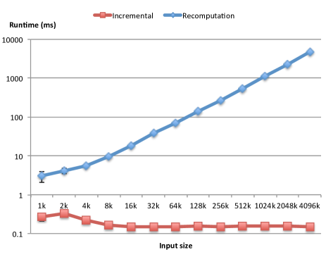
Figure 7: Performance results in log-log scale, with input size on the x-axis and runtime in ms on the y-axis. Confidence intervals are shown by the whiskers; most whiskers are simply too small to be visible.

5 Related work

Existing work on incremental computation can be divided into two groups: Static incrementalization and dynamic incrementalization. Static approaches analyze a program statically and generate an incremental version of it. Dynamic approaches create dynamic dependency graphs while the program runs and propagate changes along these graphs.

The trade-off between the two is that static approaches have the potential to be faster because no dependency tracking at runtime is needed, whereas dynamic approaches can support more powerful programming languages. The quick summary of how I$\lambda$C fits into this landscape is that it pushes the envelope with regard to the expressive power of languages whose programs can be incrementalized statically.

In the remainder of this section, we analyze the relation to the most closely related prior works. Ramalingam and Reps [1993] and Acar et al. [2006] discuss further related work.

5.1 Dynamic approaches

One of the most advanced dynamic approach to incrementalization is self-adjusting computation, which has been applied to Standard ML and large subsets of C [Acar, 2009; Hammer et al., 2011]. In this approach, programs execute on the original input in an enhanced runtime environment that tracks the dependencies between values in a dynamic dependence graph [Acar et al., 2006]; intermediate results are memoized. Later, changes to the input propagate through dependency graphs from changed inputs to results, updating both intermediate and final results; this processing is often more efficient than recomputation.

However, creating dynamic dependence graphs imposes a large constant-factor overhead during runtime, ranging from 2 to 30 in reported experiments [Acar et al., 2009, 2010], and affecting the initial run of the program on its base input. Acar et al. [2010] show how to support high-level data types in the context of self-adjusting computation; however, the approach still requires expensive runtime bookkeeping during the initial run. Like other static approaches, our work needs no modified runtime environment and has no overhead during base computation, though it may be less efficient when processing changes. This pays off if the initial input is big compared to its changes.

Chen et al. [2011] have developed a static transformation for purely functional programs, but this transformation just provides a superior inferface to use the runtime support with less boilerplate, and does not reduce this performance overhead. Hence, it is still a dynamic approach and should not be confused with the transformation we show in this work.

Another property of self-adjusting computation is that incrementalization is only efficient if the program has a suitable computation structure. For instance, a program folding the elements of a bag with a left or right fold will not have efficient incremental behavior; instead, it’s necessary that the fold be shaped like a balanced tree. In general, incremental computations become efficient only if they are stable [Acar, 2005]. Hence one may need to massage the program to make it efficient. Our methodology is different: Since we do not aim to incrementalize arbitrary programs written in standard programming languages, we can select primitives that have efficient derivatives and thereby require the programmer to use them.

Functional reactive programming [Elliott and Hudak, 1997] can also be seen as a dynamic approach to incremental computation; recent work by Maier and Odersky [2013] has focused on speeding up reactions to input changes by making them incremental on collections. Dynamic techniques are also used by Willis et al. [2008] to incrementalize JQL queries.

5.2 Static approaches

Static approaches analyze a program at compile-time and produce an incremental version that efficiently updates the output of the original program according to changing inputs.

Static approaches have the potential to be more efficient than dynamic approaches, because no bookkeeping at runtime is required. Also, the computed incremental versions can often be optimized using standard compiler techniques such as constant folding or inlining. However, none of them support first-class functions; some approaches have further restrictions.

Our aim is to apply static incrementalization to more expressive languages; in particular, I$\lambda$C supports first-class functions and an open set of base types with associated primitive operations.

5.2.1 Finite differencing

Our work and terminology is partially inspired by finite differencing [Paige and Koenig, 1982]. Paige and Koenig [1982] present derivatives for a first-order language with a fixed set of primitives. This work has inspired variants of finite differencing for queries on relational data, such as algebraic differencing [Gupta and Mumick, 1999], and delta processing [Koch, 2010].

However, most work in the database community is specialized to relational databases, hence does not support nested data (either nested collections, or algebraic data types). Incremental support is further designed monolithically for a whole language, rather than piecewise. The languages that are considered do not support first-class functions.

More general (non-relational) data types are considered in the work by Gluche et al. [1997]; our support for bags and the use of groups is inspired by their work, but their architecture is still rather restrictive: they lack support for function changes and restrict incrementalization to self-maintainable views.

5.2.2 Static memoization

Liu [2000]’s work allows to incrementalize a first-order base program $f(x_{\textrm{old}})$ to compute $f(x_{\textrm{new}})$, knowing how $x_{\textrm{new}}$ is related to $x_{\textrm{old}}$. To this end, they transform $f(x_{\textrm{new}})$ into an incremental program which reuses the intermediate results produced while computing $f(x_{\textrm{old}})$, the base program. To this end, (i) first the base program is transformed to save all its intermediate results, then (ii) the incremental program is transformed to reuse those intermediate results, and finally (iii) intermediate results which are not needed are pruned from the base program. However, to reuse intermediate results, the incremental program must often be rearranged, using some form of equational reasoning, into some equivalent program where partial results appear literally. For instance, if the base program $f$ uses a left fold to sum the elements of a list of integers $x_{\textrm{old}}$, accessing them from the head onwards, and $x_{\textrm{new}}$ prepends a new element $h$ to the list, at no point does $f(x_{\textrm{new}})$ recompute the same results. But since addition is commutative on integers, we can rewrite $f(x_{\textrm{new}})$ as $f(x_{\textrm{old}})+h$. The author’s CACHET system will try to perform such rewritings automatically, but it is not guaranteed to succeed. Similarly, CACHET will try to synthesize any additional results which can be computed cheaply by the base program to help make the incremental program more efficient.

Since it is hard to fully automate such reasoning, we move equational reasoning to the plugin design phase. A plugin provides general-purpose higher-order primitives for which the plugin authors have devised efficient derivatives (by using equational reasoning in the design phase). Then, the differentiation algorithm computes incremental versions of user programs without requiring further user intervention. It would be useful to combine I$\lambda$C with some form of static caching to make the computation of derivatives which are not self-maintainable more efficient. We plan to do so in future work.

6 Conclusions and future work

We have presented I$\lambda$C, an approach to lifting incremental computations on first-order programs to incremental computations on higher-order programs. We have presented a machine-checked correctness proof of a formalization of I$\lambda$C and an initial experimental evaluation in the form of an implementation, a sample plugin for maps and bags, and a non-trivial example that was incrementalized successfully and efficiently.

Our work opens several avenues of future work. Our current implementation is not very efficient on derivatives that are not self-maintainable. However, as discussed (Sec. 4.3), we plan to investigate approaches to memoizing intermediate results to address this limitation. Our next step will be to develop language plugins which have efficient non-self-maintainable primitives.

Another area of future work is adding support for algebraic data types (including recursive types), polymorphism, subtyping, general recursion and other collection types. While support for algebraic data types could subsume support for specific collections, many collections have additional algebraic properties that enable faster incrementalization (like bags). Even lists (which have fewer algebraic properties) can benefit from special support [Maier and Odersky, 2013].

Finally, we intend to perform a full and thorough experimental evaluation to demonstrate that I$\lambda$C can incrementalize large-scale practical programs.

We would like to thank Sebastian Erdweg, Ingo Maier, Erik Ernst, Tiark Rompf, and other ECOOP 2013 participants for helpful discussions. This work is supported by the European Research Council, grant #203099 “ScalPL”.

References

- Acar [2005] U. A. Acar. Self-Adjusting Computation. PhD thesis, Princeton University, 2005.
- Acar [2009] U. A. Acar. Self-adjusting computation: (an overview). In PEPM, pages 1–6. ACM, 2009.
- Acar et al. [2006] U. A. Acar, G. E. Blelloch, and R. Harper. Adaptive functional programming. TOPLAS, 28(6):990–1034, Nov. 2006.
- Acar et al. [2009] U. A. Acar, G. E. Blelloch, M. Blume, R. Harper, and K. Tangwongsan. An experimental analysis of self-adjusting computation. TOPLAS, 32(1):3:1–3:53, Nov. 2009.
- Acar et al. [2010] U. A. Acar, G. Blelloch, R. Ley-Wild, K. Tangwongsan, and D. Turkoglu. Traceable data types for self-adjusting computation. In PLDI, pages 483–496. ACM, 2010.
- Agda Development Team [2013] Agda Development Team. The Agda Wiki. http://wiki.portal.chalmers.se/agda/, 2013. Accessed on 2013-10-30.
- Appel and Jim [1997] A. W. Appel and T. Jim. Shrinking lambda expressions in linear time. JFP, 7:515–540, 1997.
- Chen et al. [2011] Y. Chen, J. Dunfield, M. A. Hammer, and U. A. Acar. Implicit self-adjusting computation for purely functional programs. In ICFP, pages 129–141. ACM, 2011.
- Elliott and Hudak [1997] C. Elliott and P. Hudak. Functional reactive animation. In ICFP, pages 263–273. ACM, 1997.
- Georges et al. [2007] A. Georges, D. Buytaert, and L. Eeckhout. Statistically rigorous Java performance evaluation. In OOPSLA, pages 57–76. ACM, 2007.
- Gluche et al. [1997] D. Gluche, T. Grust, C. Mainberger, and M. Scholl. Incremental updates for materialized OQL views. In Deductive and Object-Oriented Databases, volume 1341 of LNCS, pages 52–66. Springer, 1997.
- Gupta and Mumick [1999] A. Gupta and I. S. Mumick. Maintenance of materialized views: problems, techniques, and applications. In A. Gupta and I. S. Mumick, editors, Materialized views, pages 145–157. MIT Press, 1999.
- Hammer et al. [2011] M. A. Hammer, G. Neis, Y. Chen, and U. A. Acar. Self-adjusting stack machines. In OOPSLA, pages 753–772. ACM, 2011.
- Koch [2010] C. Koch. Incremental query evaluation in a ring of databases. In Proc. Symp. Principles of Database Systems (PODS), pages 87–98. ACM, 2010.
- Lämmel [2007] R. Lämmel. Google’s MapReduce programming model — revisited. Sci. Comput. Program., 68(3):208–237, Oct. 2007.
- Liu [2000] Y. A. Liu. Efficiency by incrementalization: An introduction. HOSC, 13(4):289–313, 2000.
- Maier and Odersky [2013] I. Maier and M. Odersky. Higher-order reactive programming with incremental lists. In ECOOP, pages 707–731. Springer-Verlag, 2013.
- Mitchell [1996] J. C. Mitchell. Foundations of programming languages. MIT Press, 1996.
- Paige and Koenig [1982] R. Paige and S. Koenig. Finite differencing of computable expressions. TOPLAS, 4(3):402–454, July 1982.
- Ramalingam and Reps [1993] G. Ramalingam and T. Reps. A categorized bibliography on incremental computation. In POPL, pages 502–510. ACM, 1993.
- Rompf and Odersky [2010] T. Rompf and M. Odersky. Lightweight modular staging: a pragmatic approach to runtime code generation and compiled DSLs. In GPCE, pages 127–136. ACM, 2010.
- Salvaneschi and Mezini [2013] G. Salvaneschi and M. Mezini. Reactive behavior in object-oriented applications: an analysis and a research roadmap. In AOSD, pages 37–48. ACM, 2013.
- Willis et al. [2008] D. Willis, D. J. Pearce, and J. Noble. Caching and incrementalisation in the Java Query Language. In OOPSLA, pages 1–18. ACM, 2008.