Homogenization of the one-dimensional wave equation

Abstract

We present a method for two-scale model derivation of the periodic homogenization of the one-dimensional wave equation in a bounded domain. It allows for analyzing the oscillations occurring on both microscopic and macroscopic scales. The novelty reported here is on the asymptotic behavior of high frequency waves and especially on the boundary conditions of the homogenized equation. Numerical simulations are reported.

Keywords. Homogenization, Bloch waves, wave equation, two-scale transform.

1 Introduction

The paper is devoted to the periodic homogenization of the wave equation in a one-dimensional open bounded domain where the time-independent coefficients are $\varepsilon-$periodic with small period $\varepsilon>0$. Corrector results for the low frequency waves have been published in [2, 4]. These works were not taking into account fast time oscillations, so the models reflect only a part of the physical solution. In [3], an homogenized model has been developed to cover the time and space oscillations occurring both at low and high frequencies. Unfortunately, the boundary conditions of the homogenized model was not found. Therefore, establishing the boundary conditions of the homogenized model is critical and is the goal of the present work which also extends [5].

To this end, the wave equation is written under the form of a first order formulation and the modulated two-scale transform $W_{k}^{\varepsilon}$ is applied to the solution $U^{\varepsilon}$ as in [3]. For $n\in\mathbb{N}^{\ast}$ and $k\in\mathbb{R},$ the $n^{th}$ eigenvalue $\lambda_{n}^{k}$ of the Bloch wave problem with $k$-quasi-periodic boundary conditions satisfies $\lambda_{n}^{k}=\lambda_{n}^{-k}$, in addition $\lambda_{m}^{k}=\lambda_{n}^{k}$ for $k\in\mathbb{Z}/2$, so the corresponding waves are oscillating with the same frequency. The homogenized model is thus derived for pairs of fibers $\{-k,k\}$ if $k\neq 0$ and for fiber $\left\{0\right\}$ otherwise which allows to derive the expected boundary conditions. The weak limit of $\sum\nolimits_{\sigma\in\left\{-k,k\right\}}W_{\sigma}^{\varepsilon}U^{\varepsilon}$ includes low and high frequency waves, the former being solution of the homogenized model derived in [2, 4] and the latter are associated to Bloch wave expansions. Numerical results comparing solutions of the wave equation with solution of the two-scale model for fixed $\varepsilon$ and $k$ are reported in the last section.

2 The physical problem and elementary properties

The physical problem We consider $I=\left(0,T\right)\subset\mathbb{R}^{+}$ a finite time interval and $\Omega=\left(0,\alpha\right)\subset\mathbb{R}^{+}$ a space interval, which boundary is denoted by $\partial\Omega$. Here, as usual $\varepsilon>0$ denotes a small parameter intended to go to zero. Two functions $\left(a^{\varepsilon},\rho^{\varepsilon}\right)$ are assumed to obey a prescribed profile $a^{\varepsilon}:=a\left({\frac{x}{\varepsilon}}\right)$ and $\rho^{\varepsilon}:=\rho\left({\frac{x}{\varepsilon}}\right)$ where $\rho\in L^{\infty}\left(\mathbb{R}\right)$, $a\in W^{1,\infty}\left(\mathbb{R}\right)$ are both $Y-$periodic where $Y=\left(0,1\right)$. Moreover, they are required to satisfy the standard uniform positivity and ellipticity conditions, $0<\rho^{0}\leq\rho\leq\rho^{1}$ and $0<a^{0}\leq a\leq a^{1},$ for some given strictly positive numbers $\rho^{0}$, $\rho^{1}$, $a^{0}$ and $a^{1}$. We consider $u^{\varepsilon}\left(t,x\right)$ solution to the wave equation with the source term $f^{\varepsilon}\in L^{2}\left(I\times\Omega\right)$, initial conditions $(u_{0}^{\varepsilon},v_{0}^{\varepsilon})\in L^{2}\left(\Omega\right)^{2}$ and homogeneous Dirichlet boundary conditions,

$$\begin{array}[]{l}\rho^{\varepsilon}\partial_{tt}{u^{\varepsilon}}-{\partial_{x}}\left({{a^{\varepsilon}}{\partial_{x}}u^{\varepsilon}}\right)={f^{\varepsilon}}\,\ \text{in}\,\ I\times\Omega,\\ {u^{\varepsilon}}\left({t=0,.}\right)=u_{0}^{\varepsilon}\,\ \text{and}\,\ {\partial_{t}}{u^{\varepsilon}}\left({t=0,.}\right)=v_{0}^{\varepsilon}\ \text{in}\,\ \Omega,\\ {u^{\varepsilon}}={0}\,\ \text{on}\,\ I\times\partial\Omega.\end{array}$$ (1)

By setting: ${U^{\varepsilon}}:=({\sqrt{{a^{\varepsilon}}}{\partial_{x}}{u^{\varepsilon},}\sqrt{{\rho^{\varepsilon}}}{\partial_{t}}{u^{\varepsilon})}},$ ${A^{\varepsilon}}=\left({\begin{array}[]{cc}0&{\sqrt{{a^{\varepsilon}}}{\partial_{x}}\left({\frac{1}{\sqrt{{\rho^{\varepsilon}}}}.}\right)}\\ {\frac{1}{\sqrt{{\rho^{\varepsilon}}}}{\partial_{x}}\left({\sqrt{{a^{\varepsilon}}}.}\right)}&0\end{array}}\right),\,$ $U_{0}^{\varepsilon}:=({\sqrt{{a^{\varepsilon}}}{\partial_{x}}u_{0}^{\varepsilon},\sqrt{{\rho^{\varepsilon}}}v_{0}^{\varepsilon})}$ and ${F^{\varepsilon}}:=(0,{{f^{\varepsilon}/}}\sqrt{{\rho^{\varepsilon}}})$, we reformulate the wave equation (1) as an equivalent system,

$$\left({{\partial_{t}}-{A^{\varepsilon}}}\right){U^{\varepsilon}}={F^{\varepsilon}}\text{ in }I\times\Omega,{U^{\varepsilon}}\left({t=0}\right)=U_{0}^{\varepsilon}\text{ in }\Omega\text{ and }{{{U_{2}^{\varepsilon}}}}={0}\text{ on }I\times\partial\Omega$$

where ${{{U_{2}^{\varepsilon}}}}$ is the second component of $U^{\varepsilon}$. From now on, this system will be referred to as the physical problem and taken in the distributional sense,

$$\int\nolimits_{I\times\Omega}{{F^{\varepsilon}}\cdot{\Psi\,}+{U^{\varepsilon}}\cdot\left({{\partial_{t}}-{A^{\varepsilon}}}\right)\,\Psi dtdx}+\int\nolimits_{\Omega}{U_{0}^{\varepsilon}\cdot\Psi\left({t=0}\right)\,dx}=0,$$ (2)

for all the admissible test functions ${\Psi\in{H^{1}}{{\left({I\times\Omega}\right)}^{2}}}$ such that ${{\Psi\left({t,.}\right)\in D\left({{A^{\varepsilon}}}\right)}}$ for a.e. ${t\in I}$ where the domain $D(A^{\varepsilon}):=\{{\left({\varphi,\phi}\right)\in{L^{2}}\left(\Omega\right)}^{2}|{{\sqrt{{a^{\varepsilon}}}\varphi\in{H^{1}}\left(\Omega\right),}}$ ${{{\phi/\rho}\in{H_{0}^{1}}\left(\Omega\right)}\}}$. As proved in [3], the operator $iA^{\varepsilon}$ with the domain $D(A^{\varepsilon})$ is self-adjoint on $L^{2}(\Omega)^{2}$. We assume that the data are bounded ${\left\|{f^{\varepsilon}}\right\|_{{L^{2}}\left({I\times\Omega}\right)}}+{\left\|{{\partial_{x}}u_{0}^{\varepsilon}}\right\|_{{L^{2}}\left(\Omega\right)}}+{\left\|{v_{0}^{\varepsilon}}\right\|_{{L^{2}}\left(\Omega\right)}}\leq c_{0}$, then $U^{\varepsilon}$ is uniformly bounded in ${L^{2}}\left({I\times\Omega}\right).$

Bloch waves We introduce the dual $Y^{\ast}=\left(-\frac{1}{2},\frac{1}{2}\right)$ of $Y$. For any $k\in Y^{\ast}$, we define the space of $k-$quasi-periodic functions $L_{k}^{2}:=\{u\in L_{loc}^{2}(\mathbb{R})$ ${|}$ $u(x+\ell)=u(x)e^{2i\pi k\ell}$ a.e. in $\mathbb{R}$ for all $\ell\in\mathbb{Z}\}$ and set $H_{k}^{s}:=L_{k}^{2}\cap H_{loc}^{s}\left(\mathbb{R}\right)$ for $s\geq 0.$ The periodic functions correspond to $k=0$. For a given $k\in Y^{\ast}$, we denote by $(\lambda_{n}^{k},\phi_{n}^{k})_{n\in\mathbb{N}^{\ast}}$ the Bloch wave eigenelements that are solution to

$$\mathcal{P}(k):-\partial_{y}\left(a\partial_{y}\phi_{n}^{k}\right)=\lambda_{n}^{k}\rho\phi_{n}^{k}\text{ in }Y\text{ with }\phi_{n}^{k}\in H_{k}^{2}(Y)\text{ and }\left\|\phi_{n}^{k}\right\|_{L^{2}\left(Y\right)}=1.$$

The asymptotic spectral problem $\mathcal{P}(k)$ is also restated as a first order system by setting $A_{k}:=\left({\begin{array}[]{cc}0&{\sqrt{a}\partial_{y}\left(\frac{1}{\sqrt{\rho}}.\right)}\\ \frac{1}{\sqrt{\rho}}{\partial_{y}\left({\sqrt{a}.}\right)}&0\end{array}}\right)$, $n_{A_{k}}=\frac{1}{\sqrt{\rho}}\left(\begin{array}[]{cc}0&{\sqrt{a}n}_{Y}\\ {\sqrt{a}n}_{Y}&0\end{array}\right)$ and $e_{n}^{k}:=\frac{1}{\sqrt{2}}\left(\begin{array}[]{c}-i{s_{n}/\sqrt{\lambda_{\left|n\right|}^{k}}}\sqrt{a}\partial_{y}\left({\phi_{\left|n\right|}^{k}}\right)\\ \sqrt{\rho}\phi_{\left|n\right|}^{k}\end{array}\right)$ where $s_{n}$ and $n_{Y}$ denote the sign of $n\in\mathbb{Z}^{\ast}$ and the outer unit normal of $\partial Y$ respectively. As proved in [3], $iA_{k}$ is self-adjoint on the domain $D\left({A_{k}}\right):=\{{\left({\varphi,\phi}\right)\in L^{2}\left(Y\right)^{2}|\sqrt{a}\varphi\in H_{k}^{1}\left(Y\right),}$ ${{\phi/}\sqrt{\rho}\in H_{k}^{1}\left(Y\right)}\subset L^{2}\left(Y\right)^{2}\}.$ The Bloch wave spectral problem $\mathcal{P(}k\mathcal{)}$ is equivalent to finding pairs $\left(\mu_{n}^{k},e_{n}^{k}\right)$ indexed by $n\in\mathbb{Z}^{\ast}$ solution to $\mathcal{Q(}k\mathcal{)}:A_{k}e_{n}^{k}=is_{n}\sqrt{\lambda_{\left|n\right|}^{k}}e_{n}^{k}$  in $Y$ with $e_{n}^{k}\in H_{k}^{1}\left(Y\right)^{2}$. We pose $M_{n}^{k}:=\{m{\in{\mathbb{Z}}}^{\ast}{|}\lambda_{m}^{k}{=}\lambda_{n}^{k}$ and $s_{m}=s_{n}\}$ and introduce the coefficients $b(k,n,m)=\int_{Y}\rho\phi_{\left|n\right|}^{k}\cdot\phi_{\left|m\right|}^{k}dy$ and $c(k,n,m)=i{s_{n}/}\left({2\sqrt{\lambda_{\left|n\right|}^{k}}}\right)\int_{Y}{\phi_{\left|n\right|}^{k}\cdot a{{\partial_{y}}}\phi_{\left|m\right|}^{k}}-a\partial_{y}{\phi_{\left|n\right|}^{k}}\cdot{\phi_{\left|m\right|}^{k}}dy$ for $n,m\in M_{n}^{k}.$

The modulated two-scale transform Let us assume from now that the domain $\Omega$ is the union of a finite number of entire cells of size $\varepsilon$ or equivalently that the sequence $\varepsilon$ is exactly $\varepsilon_{n}=\frac{\alpha}{n}$ for $n\in\mathbb{N}^{\ast}$. For any $k\in Y^{\ast}$, we define $I^{k}=\left\{-k,k\right\}$ if $k\neq 0$ and $I^{0}=\left\{0\right\}$. By choosing $\Lambda=\left(0,1\right)$ as a time unit cell, we introduce the operator $W_{k}^{\varepsilon}:L^{2}\left(I\times\Omega\right)^{2}\rightarrow L^{2}\left(I\times\Lambda\times\Omega\times Y\right)^{2}$ acting in all time and space variables,

$$W_{k}^{\varepsilon}:=\left(1-\sum\nolimits_{n\in\mathbb{Z}^{\ast}}\Pi_{n}^{k}\right)S_{k}^{\varepsilon}+\sum\nolimits_{n\in\mathbb{Z}^{\ast}}{{T^{\varepsilon\alpha_{n}^{k}}\Pi}}_{n}^{k}{S_{k}^{\varepsilon}}$$ (3)

where the time and space two-scale transforms ${{T^{\varepsilon\alpha_{n}^{k}}}}$ and ${S_{k}^{\varepsilon}}$, and the orthogonal projector $\Pi_{n}^{k}$ onto $e_{n}^{k}$ are defined in [3], see pages 11,15 and 17, with $\alpha_{n}^{k}=2\pi/\sqrt{\lambda_{n}^{k}}$, and where it is proved that,

$$\left\|W_{k}^{\varepsilon}u\right\|_{L^{2}\left(I\times\Lambda\times\Omega\times Y\right)}^{2}=\left\|u\right\|_{L^{2}\left(I\times\Omega\right)}^{2}.$$ (4)

We define $(\mathfrak{B}_{n}^{k}v)(t,x)=v(t,\frac{t}{\varepsilon\alpha_{n}^{k}},x,\frac{x}{\varepsilon})$ the operator that operates on functions $v(t,{\tau},x,y)$ defined in $I\times\mathbb{R\times}\Omega\times\mathbb{R}$. The notation $O\left(\varepsilon\right)$ refers to numbers or functions tending to zero when $\varepsilon\rightarrow 0$ in a sense made precise in each case. The next Lemma shows that $\mathfrak{B}_{n}^{k}$ is an approximation of $T^{\varepsilon\alpha_{n}^{k}\ast}S_{k}^{\varepsilon\ast}$ for a function which is periodic in $\tau$ and $k-$quasi-periodic in $y$, where $T^{\varepsilon\alpha_{n}^{k}\ast}:L^{2}\left(I\times\Lambda\right)\rightarrow L^{2}\left(I\right)$ and $S_{k}^{\varepsilon\ast}:L^{2}\left(\Omega\times Y\right)\rightarrow L^{2}\left(\Omega\right)$ are adjoint of $T^{\varepsilon\alpha_{n}^{k}}$ and $S_{k}^{\varepsilon}$ respectively.

Lemma 2.1.

Let $v\in C^{1}\left(I\times\Lambda\times\Omega\times Y\right)$ a periodic function in $\tau$ and $k-$quasi-periodic in $y$, then $T^{\varepsilon\alpha_{n}^{k}\ast}S_{k}^{\varepsilon\ast}v=\mathfrak{B}_{n}^{k}v+O\left(\varepsilon\right)$ in the $L^{2}\left(I\times\Omega\right)$ sense. Consequently, for any sequence $u^{\varepsilon}$ bounded in $L^{2}\left(I\times\Omega\right)$ such that $T^{\varepsilon\alpha_{n}^{k}}S_{k}^{\varepsilon}u^{\varepsilon}$ converges to $u$ in $L^{2}(I\times\Lambda\times\Omega\times Y)$ weakly when $\varepsilon\rightarrow 0$,

$$\int_{I\times\Omega}u^{\varepsilon}\cdot\mathfrak{B}_{n}^{k}v\text{ }dtdx\rightarrow\int_{I\times\Lambda\times\Omega\times Y}u\cdot v\text{ }dtd\tau dxdy\text{ \ when }\varepsilon\rightarrow 0.$$ (5)

Note that for $k=0$, the convergence (5) regarding each variable corresponds to the definition of two-scale convergence in [1]. The proof is carried out in three steps. First the explicit expression of $T^{\varepsilon\alpha_{n}^{k}\ast}S_{k}^{\varepsilon\ast}v$ is derived, second the approximation of $T^{\varepsilon\alpha_{n}^{k}\ast}S_{k}^{\varepsilon\ast}v$ is deduced, finally the convergence (5) follows. For a function $v\left(t,\tau,x,y\right)$ defined in $I\times\Lambda\times\Omega\times Y,$ we observe that

$$A^{\varepsilon}\mathfrak{B}_{n}^{k}v=\mathfrak{B}_{n}^{k}\left(\left(\frac{A_{k}}{\varepsilon}+B\right)v\right)\text{ and }{{\partial_{t}}}\left({\mathfrak{B}}_{n}^{k}v\right)={\mathfrak{B}}_{n}^{k}\left(\left(\frac{\partial_{\tau}}{\varepsilon\alpha_{n}^{k}}+\partial_{t}\right)v\right)\text{,}$$ (6)

where the operator $B$ is defined as the result of the formal substitution of $x-$derivatives by $y-$derivatives in $A_{k}$.

3 Homogenized results and their proof

For $k\in Y^{\ast}$, we decompose

$$\frac{\alpha k}{\varepsilon}=h_{\varepsilon}^{k}+l_{\varepsilon}^{k}\text{ with }h_{\varepsilon}^{k}=\left[\frac{\alpha k}{\varepsilon}\right]\text{ and }l_{\varepsilon}^{k}\in\left[0,1\right),$$ (7)

and assume that the sequence $\varepsilon$ is varying in a set $E_{k}\subset\mathbb{R}^{+\ast}$ depending on $k$ so that

$$l_{\varepsilon}^{k}\rightarrow l^{k}\text{ when }\varepsilon\rightarrow 0\text{ and }\varepsilon\in E_{k}\text{ with }l^{k}\in\left[0,1\right).$$ (8)

We note that for $k=0$, $h_{\varepsilon}^{k}=0,$ $l_{\varepsilon}^{k}=0$, so $l^{k}=0$ and $E_{0}=\mathbb{R}^{+\ast}$. After extraction of a subsequence, we introduce the weak limits of the relevant projections along $e_{n}^{k}$ for any $n\in{\mathbb{Z}}^{\ast}$,

$$F_{n}^{k}:=\lim_{\varepsilon\rightarrow 0}\int\nolimits_{\Lambda\times Y}{T}^{\varepsilon\alpha_{n}^{k}}{S{{}_{k}^{\varepsilon}{F^{\varepsilon}}\cdot{e^{2i\pi{s_{n}}\tau}}e_{n}^{k}dyd\tau}}\text{ and }U_{0,n}^{k}:=\lim_{\varepsilon\rightarrow 0}\int\nolimits_{Y}{S_{k}^{\varepsilon}U_{0}^{\varepsilon}\cdot e_{n}^{k}dy}.$$ (9)

The next lemmas state the microscopic equation for each mode and the corresponding macroscopic equation.

Lemma 3.1.

For $k\in Y^{\ast}$ and $n\in{\mathbb{Z}}^{\ast}$, let $U^{\varepsilon}$ be a bounded solution of (2), there exists at least a subsequence of $T^{\varepsilon\alpha_{n}^{k}}{{S}_{k}^{\varepsilon}U^{\varepsilon}}$ converging weakly towards a limit $U_{n}^{k}$ in $L^{2}(I\times\Lambda\times\Omega\times Y)^{2}$ when $\varepsilon$ tends to zero. Then $U_{n}^{k}$ is a solution of the weak formulation of the microscopic equation

$$\left(\frac{{{\partial_{\tau}}}}{\alpha_{n}^{k}}{-A}_{k}\right)U_{n}^{k}=0\text{ in }I\times\Lambda\times\Omega\times Y$$ (10)

and is periodic in $\tau$ and $k-$quasi-periodic in $y$. Moreover, it can be decomposed as

$$U_{n}^{k}\left(t,\tau,x,y\right)={\sum\limits_{p\in\mathbb{M}_{n}^{k}}}u_{p}^{k}\left(t,x\right)e^{{2{i\pi s}}_{p}\tau}e_{p}^{k}\left(y\right)\text{ with }u_{p}^{k}\in L^{2}\left(I\times\Omega\right).$$ (11)

Lemma 3.2.

For each $k\in Y^{\ast}$, $n\in{\mathbb{Z}}^{\ast}$, for each $\sigma\in I^{k}$ and $q\in M_{n}^{\sigma}$, the macroscopic equation is stated by

$$\begin{array}[]{l}\sum\limits_{p\in{M}_{n}^{\sigma}}b\left(\sigma,p,q\right){\partial_{t}}u_{p}^{\sigma}-\sum\limits_{p\in{M}_{n}^{\sigma}}c\left(\sigma,p,q\right){\partial_{x}}u_{p}^{\sigma}=F_{q}^{\sigma}\,\ \text{in}\,\ I\times\Omega,\\ \sum\limits_{p\in{M}_{n}^{\sigma}}b\left(\sigma,p,q\right)u_{p}^{\sigma}\left({t=0}\right)=U_{0,q}^{\sigma}\,\ \text{in}\,\ \Omega,\end{array}$$ (12)

with the boundary conditions in case where there exist $p\in{M}_{n}^{k}$ such that $c\left(k,p,q\right)\neq 0$ and $\phi_{\left|p\right|}^{k}(0)\neq 0$

$$\sum\limits_{\sigma\in I^{k}}\sum\limits_{p\in{M}_{n}^{\sigma}}u_{p}^{\sigma}\phi_{\left|p\right|}^{\sigma}\left(0\right){e^{sign\left(\sigma\right)2i\pi\frac{l^{k}x}{\alpha}}}=0\,\ \text{on}\,\ I\times\partial\Omega.$$ (13)

The low frequency part $U_{H}^{0}$ relates to the weak limit in $L^{2}\left(I\times\Omega\times Y\right)^{2}$ of the kernel part of $S_{k}^{\varepsilon}$ in 3. It has been treated completely, in [2, 3]. Here, we focus on the non-kernel part of $S_{k}^{\varepsilon}$, it relates to the high frequency waves and microscopic and macroscopic scales. In order to obtain the solution of the model, we analyze the asymptotic behaviour of each mode through ${{T^{\varepsilon\alpha_{n}^{k}}}S_{k}^{\varepsilon}}$ as in Lemma 3.1 and Lemma 3.2. Then the full solution is the sum of all modes. We introduce the characteristic function $\chi_{0}\left(k\right)=1$ if $k=0$ and $=0$ otherwise. The main Theorem states as follows.

Theorem 3.3.

For a given  $k\in Y^{\ast}$, let $U^{\varepsilon}$ be a solution of (2) bounded in $L^{2}\left(I\times\Omega\right)$, for $\varepsilon\in E_{k},$ as in (7, 8), the limit $G_{k}$ of any weakly converging extracted subsequence of $\sum\limits_{\sigma\in I^{k}}W_{\sigma}^{\varepsilon}U^{\varepsilon}$ in $L^{2}\left(I\times\Lambda\times\Omega\times Y\right)^{2}$ can be decomposed as

$$G^{k}\left(t,\tau,x,y\right)=\chi_{0}\left(k\right)U_{H}^{0}\left(t,x,y\right)+\sum\limits_{\sigma\in I^{k}}\sum\limits_{n\in\mathbb{Z}^{\ast}}{u_{n}^{\sigma}\left({t,x}\right){e^{2i\pi{s_{n}}\tau}}e_{n}^{\sigma}\left(y\right)}$$ (14)

where $\left(u_{n}^{\sigma}\right)_{n,\sigma}$ are solutions of the macroscopic equation (12, 13).

Thus, it follows from (14) that the physical solution $U^{\varepsilon}$ is approximated by two-scale modes

$$U^{\varepsilon}\left(t,x\right)\simeq\chi_{0}\left(k\right)U_{H}^{k}\left(t,x,\frac{x}{\varepsilon}\right)+\sum\nolimits_{\sigma\in I^{k}}\sum\nolimits_{n\in\mathbb{Z}^{\ast}}u_{n}^{\sigma}\left(t,x\right)e^{is_{n}\sqrt{\lambda_{n}^{\sigma}}t/\varepsilon}e_{n}^{\sigma}\left(\frac{x}{\varepsilon}\right).$$ (15)

The remain of this section provides the proofs of results.

Proof of Lemma 3.1. The test functions of the weak formulation (2) are chosen as $\Psi^{\varepsilon}=\mathfrak{B}_{n}^{k}\Psi\left({t,x}\right)$ for $k\in Y^{\ast}$, $n\in\mathbb{Z}^{\ast}$ where $\Psi\in{C^{\infty}}\left(I\times\Lambda\right.$$\left.\times\Omega\times Y\right)^{2}$ is periodic in $\tau$ and $k-$quasi-periodic in $y$. From (6) multiplied by $\varepsilon$, since ${\left({\frac{{{\partial_{\tau}}}}{{\alpha_{n}^{k}}}-{A_{k}}}\right)\Psi}$ is periodic in $\tau$ and $k-$quasi-periodic in $y$ and ${T^{\varepsilon\alpha_{n}^{k}}S_{k}^{\varepsilon}{U^{\varepsilon}\rightarrow U}}_{n}^{k}$ in $L^{2}\left(I\times\Lambda\times\Omega\times Y\right)^{2}$ weakly, Lemma 2.1 allows to pass to the limit in the weak formulation, $\int\nolimits_{I\times\Lambda\times\Omega\times Y}{U}_{n}^{k}{\cdot\left(\frac{{{\partial_{\tau}}}}{{\alpha_{n}^{k}}}{-}A_{k}\right)\Psi dtd\tau dxdy}=0$. Using the assumption $U_{n}^{k}\in D\left(A_{k}\right)\cap L^{2}\left(I\times\Omega\times Y;H^{1}\left(\Lambda\right)\right)$ and applying an integration by parts,

$$\int\nolimits_{I\times\Lambda\times\Omega\times Y}\left(-\frac{{{\partial_{\tau}}}}{{\alpha_{n}^{k}}}+A_{k}\right){U}_{n}^{k}{\cdot{\Psi}dtd\tau dxdy+}\int_{{I\times\partial\Lambda\times\Omega\times Y}}U_{n}^{k}\cdot\Psi{dtd\tau dxdy}$$

$$-\int_{{I\times\Lambda\times\Omega\times\partial Y}}U_{n}^{k}\cdot n_{A_{k}}\Psi{dtd\tau dxdy}=0.$$

Then, choosing ${\Psi\in L}^{2}\left(I\times\Omega;H_{0}^{1}\left(\Lambda\times Y\right)\right)$ comes the strong form (10). Since the product of a periodic function by a $k-$quasi-periodic function is $k-$quasi-periodic then $n_{A_{k}}\Psi$ is $k-$quasi-periodic in $y$. Therefore, $U_{n}^{k}$ is periodic in $\tau$ and $k-$quasi-periodic in $y.$ Moreover, (11) is obtained, by projection.

Proof of Lemma 3.2 For $k\in Y^{\ast}$, let $\left(\lambda_{p}^{\sigma},e_{p}^{\sigma}\right)_{p\in M_{n}^{\sigma},\sigma\in I^{k}}$ be the Bloch eigenmodes of the spectral equation $\mathcal{Q}\left(\sigma\right)$ corresponding to the eigenvalue $\lambda_{n}^{k}$. We pose $\Psi^{\varepsilon}\left(t,x\right)=\sum\nolimits_{\sigma\in I^{k}}{\mathfrak{B}}_{n}^{k}\Psi_{\varepsilon}^{\sigma}\in H^{1}\left(I\times\Omega\right)^{2}$ as a test function in the weak formulation (2) with each $\Psi_{\varepsilon}^{\sigma}\left(t,\tau,x,y\right)=\sum\nolimits_{q\in M_{n}^{k}}\varphi_{q,\varepsilon}^{\sigma}\left(t,x\right)e^{2i\pi s_{q}\tau}e_{q}^{\sigma}\left(y\right)$ where $\varphi_{q,\varepsilon}^{\sigma}\in H^{1}\left(I\times\Omega\right)$ and satisfies the boundary conditions

$\sum\nolimits_{\sigma\in I^{k},q\in M_{n}^{\sigma}}e^{2i\pi s_{q}t/(\varepsilon\alpha_{q}^{\sigma})}\varphi_{q,\varepsilon}^{\sigma}\left(t,x\right)\phi_{\left|q\right|}^{\sigma}\left(\frac{x}{\varepsilon}\right)=O\left(\varepsilon\right)$ on $I\times\partial\Omega.$ Note that this condition is related to the second component of $\Psi^{\varepsilon}$ only. Since $\alpha_{q}^{\sigma}=\alpha_{n}^{k}$ and $s_{q}=s_{n}$ for all $q\in M_{n}^{\sigma}$ and $\sigma\in I^{k}$, so $e^{2i\pi s_{q}t/(\varepsilon\alpha_{q}^{\sigma})}\neq 0$ can be eliminated. Extracting a subsequence $\varepsilon\in E_{k}$, using the $\sigma-$quasi-periodicity of $\phi_{\left|q\right|}^{\sigma}$ and (7,8), $\varphi_{q,\varepsilon}^{\sigma}$ converges strongly to some $\varphi_{q}^{\sigma}$ in $H^{1}\left(I\times\Omega\right)$, then the boundary conditions are

$$\sum\nolimits_{\sigma\in I^{k}}\sum\nolimits_{q\in M_{n}^{\sigma}}\varphi_{q}^{\sigma}\left(t,x\right)\phi_{\left|q\right|}^{\sigma}\left(0\right)e^{sign\left(\sigma\right)2i\pi\frac{l^{k}x}{\alpha}}=0\,\text{on }I\times\partial\Omega.$$ (16)

Applying (6) and since ${\left({\frac{{{\partial_{\tau}}}}{{\alpha_{n}^{\sigma}}}-{{{A_{\sigma}}}}}\right)\Psi^{\sigma}}=0$ for $\sigma\in$ $I^{k}$, then in the weak formulation it remains

$$\sum\limits_{\sigma\in I^{k}}\int\nolimits_{I\times\Omega}{{F^{\varepsilon}\cdot\mathfrak{B}}}_{n}^{k}{{\Psi_{\varepsilon}^{\sigma}+U^{\varepsilon}}\cdot\mathfrak{B}}_{n}^{k}{\left({{\partial_{t}}-B}\right)\Psi_{\varepsilon}^{\sigma}dtdx}-\int\nolimits_{\Omega}{{U_{0}^{\varepsilon}}\cdot\mathfrak{B}}_{n}^{k}{\Psi_{\varepsilon}^{\sigma}}\left(t=0\right){dx=0}.$$

Since ${\left({{\partial_{t}}-B}\right)\Psi_{\varepsilon}^{\sigma}}$ is $\sigma-$quasi-periodic, so passing to the limit thanks to Lemma 2.1, after using (9) and replacing the decomposition of $U_{n}^{\sigma}$,

$$\sum\limits_{\sigma\in I^{k},\{p,q\}\in M_{n}^{\sigma}}\left(\int\nolimits_{I\times\Omega}b\left(\sigma,p,q\right)u_{p}^{\sigma}\cdot{\partial}_{t}\varphi_{q}^{\sigma}-{c}\left(\sigma,p,q\right){{u_{p}^{\sigma}\cdot{{\partial_{x}}}}\varphi_{q}^{\sigma}-F_{q}^{\sigma}}\cdot{\varphi_{q}^{\sigma}\,dtdx}\right.$$

$$\left.{-}\int_{\Omega}{U}_{0,q}^{\sigma}{\cdot\varphi_{q}^{\sigma}}\left(t=0\right){dx}\right){=0}\text{ for all }{\varphi_{q}^{\sigma}\in}H^{1}\left(I\times\Omega\right)\text{ fulfilling (\ref{boundary-test})}.$$

Moreover, if $u_{q}^{\sigma}{\in}H^{1}\left(I\times\Omega\right)$ then it satisfies the strong form of the internal equations (12) for each $\sigma\in I^{k}$, $q\in M_{n}^{\sigma}$ and the boundary conditions

$$\sum\nolimits_{\sigma,p,q}{{c\left(\sigma,p,q\right)u_{p}^{\sigma}}}\overline{\varphi_{q}^{\sigma}}=0\text{ on }I\times\partial\Omega\text{ for }\varphi_{q}^{\sigma}\text{ satisfies (\ref{boundary-test})}.$$ (17)

In order to find the boundary conditions of $\left({{u_{p}^{\sigma}}}\right)_{\sigma,p}$, we distinguish between the two cases $k\neq 0$ and $k=0$. First, for $k\neq 0$, $\lambda_{n}^{k}$ is simple so $M_{n}^{k}=\left\{n\right\}$. Introducing $C=diag\left(c\left(\sigma,n,n\right)\right)_{\sigma}$, $B=diag\left(b\left(\sigma,n,n\right)\right)_{\sigma}$, $U=\left(u_{n}^{\sigma}\right)_{\sigma}$, $F=\left(F_{n}^{\sigma}\right)_{\sigma}$, $U_{0}=\left(U_{0,n}^{\sigma}\right)_{\sigma}$, $\Psi=\left(\varphi_{n}^{\sigma}\right)_{\sigma}$, $\Phi=\left(\phi_{\left|n\right|}^{\sigma}\left(0\right)e^{sign\left(\sigma\right)2i\pi l^{k}x/\alpha}\right)_{\sigma}$, Equation (12) states under matrix form

$$B{\partial}_{t}U+C{\partial_{x}}U=F\text{ in }I\times\Omega\text{ and }BU\left(t=0\right)=U_{0}\text{ in }\Omega,$$ (18)

which boundary condition (17) is rewritten as $CU\left(t,x\right).\overline{\Psi}\left(t,x\right)=0$ on $I\times\partial\Omega$ for all $\Psi$ such that $\overline{\Phi}(x).\overline{\Psi}(t,x)=0$ on $I\times\partial\Omega.$ Equivalently, $CU\left(t,x\right)$ is collinear with $\overline{\Phi}(x)$ yielding the boundary condition $u_{n}^{k}\phi_{\left|n\right|}^{k}\left(0\right){e^{2i\pi\frac{l^{k}x}{\alpha}}}$ ${+}$ $u_{n}^{-k}\phi_{\left|n\right|}^{-k}\left(0\right){e^{-2i\pi\frac{l^{k}x}{\alpha}}}=0$ on $\ I\times\partial\Omega$ after remarking that $c\left(k,n,n\right)\neq 0$ and $c\left(k,n,n\right)=-c\left(-k,n,n\right)$.

Second, for $k=0$, $\lambda_{n}^{0}$ is double $\lambda_{n}^{0}=\lambda_{m}^{0}$ so $M_{n}^{k}=\left\{n,m\right\}$. With $C=\left(c\left(0,p,q\right)\right)_{p,q}$, $B=\left(b\left(0,p,q\right)\right)_{p,q}$, $U=\left(u_{p}^{0}\right)_{p}$, $F=\left(F_{q}^{0}\right)_{q}$, $U_{0}=\left(U_{0,q}^{0}\right)_{q}$, $\Psi=\left(\varphi_{q}^{0}\right)_{q}$, $\Phi=\left(\phi_{\left|q\right|}^{0}\left(0\right)\right)_{q}$, the matrix form is still stated as (18). Here, the eigenvectors are chosen as real functions then $c\left(0,p,p\right)=0.$ Since $c\left(0,n,m\right)\neq 0$, so the boundary condition is $u_{n}^{0}\phi_{\left|n\right|}^{0}\left(0\right){+}u_{m}^{0}\phi_{\left|m\right|}^{0}\left(0\right)=0\,\text{on}\ I\times\partial\Omega\text{.}$

Proof of Theorem For a given $k\in Y^{\ast}$, let $U^{\varepsilon}$ be solution of (2) which is bounded in $L^{2}(I\times\Omega)$, the property (4) yields the boundness of $\left\|W_{\sigma}^{\varepsilon}U^{\varepsilon}\right\|_{L^{2}\left(I\times\Lambda\times\Omega\times Y\right)}$ for $\sigma\in I^{k}$. So there exists $G^{k}\in L^{2}\left(I\times\Lambda\times\Omega\times Y\right)^{2}$ such that, up to the extraction of a subsequence, $\sum\nolimits_{\sigma\in I^{k}}W_{\sigma}^{\varepsilon}U^{\varepsilon}$ tends weakly to $G^{k}=\chi_{0}\left(k\right)U_{H}^{0}+\sum\nolimits_{\sigma\in I^{k}}\sum\nolimits_{n\in\mathbb{Z}^{\ast}}U_{n}^{k}$ in $L^{2}\left(I\times\Lambda\times\Omega\times Y\right)^{2}$. The high frequency part is based on the decomposition (11) and Lemma 3.2.

Remark 3.4.

This method allows to complete the homogenized model of the wave equation in [3] for the one-dimensional case. Let $K\in\mathbb{N}^{\ast}$, we decompose $\frac{\alpha}{\varepsilon K}=\left[\frac{\alpha}{\varepsilon K}\right]+l_{\varepsilon}^{1}$ with $l_{\varepsilon}^{1}\in[0,1)$ and assume that the sequence $\varepsilon$ is varying in a set $E_{K}\subset\mathbb{R}^{+\ast}$ depending on $K$ so that $l_{\varepsilon}^{1}\rightarrow l^{1}$ when $\varepsilon\rightarrow 0$ with $l^{1}\in[0,1)$. For any $k\in L_{K}^{\ast}$, defined in [3], we denote $p_{k}=kK\in\mathbb{N}$, so $\frac{\alpha p_{k}}{\varepsilon K}=p_{k}\left[\frac{\alpha}{\varepsilon K}\right]+p_{k}l_{\varepsilon}^{1}$ and $p_{k}l_{\varepsilon}^{1}$ $\rightarrow l^{k}:=p_{k}l^{1}$ when $\varepsilon\rightarrow 0$ with the same sequence of $\varepsilon\in E_{K}$.

4 Numerical examples

We report simulations regarding comparison of physical solution and its approximation for $I=\left(0,1\right),$ $\Omega=\left(0,1\right)$, $\rho=1$, $a=\frac{1}{3}\left(\sin\left(2\pi y\right)+2\right)$, $f^{\varepsilon}=0$,  $v_{0}^{\varepsilon}=0$, $\varepsilon=\frac{1}{10}$ and $k=0.16$. Since $k\neq 0$, so the approximation (15) comes

$$U^{\varepsilon}\left(t,x\right)\simeq\sum\nolimits_{\sigma\in I^{k}}\sum\nolimits_{n\in\mathbb{Z}^{\ast}}u_{n}^{\sigma}\left(t,x\right)e^{is_{n}\sqrt{\lambda_{n}^{\sigma}}t/\varepsilon}e_{n}^{\sigma}\left(\frac{x}{\varepsilon}\right).$$ (19)

The validation of the approximation is based on the modal decomposition of any solution $U^{\varepsilon}=\sum_{l\in\mathbb{Z}^{\ast}}R_{l}^{\varepsilon}\left(t\right)V_{l}^{\varepsilon}\left(x\right)$ where the modes $V_{l}^{\varepsilon}$ are built from the solutions $v_{l}^{\varepsilon}$ of the spectral problem $\partial_{x}\left(a^{\varepsilon}\partial_{x}v_{l}^{\varepsilon}\right)=\lambda_{l}^{\varepsilon}v_{l}^{\varepsilon}$ in $\Omega$ with $v_{l}^{\varepsilon}=0$ on $\partial\Omega$. Moreover, in [6], two-scale approximations of modes have been derived on the form of linear combinations $\sum\nolimits_{\sigma\in I^{k}}\theta_{n}^{\sigma}\left(x\right)\phi_{n}^{\sigma}\left(\frac{x}{\varepsilon}\right)$ of Bloch modes, so the initial conditions of the physical problem are taken on the form

$$u_{0}^{\varepsilon}\left(x\right)=\sum\nolimits_{n\in\mathbb{N}^{\ast}}\sum\nolimits_{\sigma\in I^{k}}\theta_{n}^{\sigma}\left(x\right)\phi_{n}^{\sigma}\left(\frac{x}{\varepsilon}\right).$$ (20)

Two simulations are reported, one for an initial condition $u_{0}^{\varepsilon}$ spanned by the pair of Bloch modes corresponding to $n=2$ when the other is spanned by three pairs $n\in\{2,3,4\}$. In the first case, the first component of $U_{0}^{\varepsilon}$ approximates the first component of a single eigenvector $V_{l}^{\varepsilon}$ approximated by (19) where all coefficients $u_{n}^{\sigma}=0$ for $n\neq\pm 2$. Fig. 1 $(a)$ shows the initial condition $u_{0}^{\varepsilon}$. Fig. 1 $(b)$ presents the real part (solid line) and the imaginary part (dashed-dotted line) of the macroscopic solution $u_{n}^{k}$ and also the real part (dotted line) and the imaginary part (dashed line) of $u_{n}^{-k}$ at space step $x=0.699$ when Fig. 1 $\left(c,d\right)$ plot the real part of the first component $U_{1}^{\varepsilon}$ of physical solution and the relative error vector of $U_{1}^{\varepsilon}$ with its approximation which $L^{2}(\Omega)$-norm is equal to 7e-3 at $t=0.466$. For the second case where $u_{n}^{\sigma}=0$ for $n\notin\{\pm 2,\pm 3,\pm 4\}$, the first component $U_{1}^{\varepsilon}$ and the relative error vector of $U_{1}^{\varepsilon}$ with its approximation which $L^{2}(\Omega)$-norm is 3.8e-3 are plotted in Fig. 1 $(e,f)$. Finally, for the two cases the $L^{2}(I)$-relative errors at $x=0.699$ on the first component are 8e-3 and 3.5e-3 respectively.

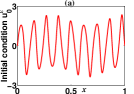
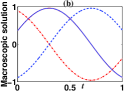
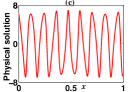
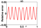
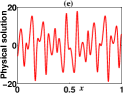
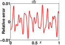
Figure 1: Numerical results

References

[1]G. Allaire, Homogenization and two-scale convergence, SIAM Journal
on Mathematical Analysis 23:6 (1992), 1482–1518.
[2]S. Brahim-Otsmane, G. Francfort, and F. Murat, Correctors for the
homogenization of the wave and heat equations, Journal de mathématiques
pures et appliquées 71:3 (1992), 197–231.
[3]M. Brassart and M. Lenczner, A two-scale model for the wave equation
with oscillating coefficients and data, Comptes Rendus Mathematique 347:23 (2009), 1439–1442.
[4]G. A. Francfort and F. Murat, Oscillations and energy densities in
the wave equation, Communications in partial differential equations 17:11-12 (1992), 1785–1865.
[5]M. Kader, Contributions à la modélisation et contrôle
des systèmes intelligents distribués: Application au contrôle de
vibrations d’une poutre, Ph.D. thesis, Université de Franche-Comté,
France, 2000.
[6]T. T. Nguyen, M. Lenczner, and M. Brassart, Homogenization of the
spectral equation in one-dimension, arXiv preprint arXiv:1310.4064 (2013).