Efficient coordinate-descent for orthogonal matrices through Givens rotations

Abstract

Optimizing over the set of orthogonal matrices is a central component in problems like sparse-PCA or tensor decomposition. Unfortunately, such optimization is hard since simple operations on orthogonal matrices easily break orthogonality, and correcting orthogonality usually costs a large amount of computation. Here we propose a framework for optimizing orthogonal matrices, that is the parallel of coordinate-descent in Euclidean spaces. It is based on Givens-rotations, a fast-to-compute operation that affects a small number of entries in the learned matrix, and preserves orthogonality. We show two applications of this approach: an algorithm for tensor decomposition that is used in learning mixture models, and an algorithm for sparse-PCA. We study the parameter regime where a Givens rotation approach converges faster and achieves a superior model on a genome-wide brain-wide mRNA expression dataset.

1 Introduction

Optimization over orthogonal matrices – matrices whose rows and columns form an orthonormal basis of $\mathbb{R}^{d}$ – is central to many machine learning optimization problems. Prominent examples include Principal Component Analysis (PCA), Sparse PCA, and Independent Component Analysis (ICA). In addition, many new applications of tensor orthogonal decompositions were introduced recently, including Gaussian Mixture Models, Multi-view Models and Latent Dirichlet Allocation (e.g., Anandkumar et al. (2012a); Hsu & Kakade (2013)).

A major challenge when optimizing over the set of orthogonal matrices is that simple updates such as matrix addition usually break orthonormality. Correcting by orthonormalizing a matrix $V\in\mathbb{R}^{d\times d}$ is typically a costly procedure: even a change to a single element of the matrix, may require $O(d^{3})$ operations in the general case for re-orthogonalization.

In this paper, we present a new approach for optimization over the manifold of orthogonal matrices, that is based on a series of sparse and efficient-to-compute updates that operate within the set of orthonormal matrices, thus saving the need for costly orthonormalization. The approach can be seen as the equivalent of coordinate descent in the manifold of orthonormal matrices. Coordinate descent methods are particularly relevant for problems that are too big to fit in memory, for problems where one might be satisfied with a partial answer, or in problems where not all the data is available at one time (Richtárik & Takáč, 2012).

We start by showing that the orthogonal-matrix equivalent of a single coordinate update is applying a single Givens rotation to the matrix. In section 3 we prove that for a differentiable objective the procedure converges to a local optimum under minimal conditions, and prove an $O(1/T)$ convergence rate for the norm of the gradient. Sections 4 and 5 describe two applications: (1) sparse PCA, including a variant for streaming data; (2) a new method for orthogonal tensor decomposition. We study how the performance of the method depends on the problems hyperparameters using synthetic data, and demonstrate that it achieves superior accuracy on an application of sparse-PCA for analyzing gene expression data.

2 Coordinate descent on the orthogonal matrix manifold

Coordinate descent (CD) is an efficient alternative to gradient descent when the cost of computing and applying a gradient step at a single coordinate is small relative to computing the full gradient. In these cases, convergence can be achieved with a smaller number of computing operations, although using a larger number of (faster) steps.

Applying coordinate descent to optimize a function involves choosing a coordinate basis, usually the standard basis. Then calculating a directional derivative in the direction of one of the coordinates. And finally, updating the iterate in the direction of the chosen coordinate.

To generalize CD to operate over the set of orthogonal matrices, we need to generalize these ideas of directional derivatives and updating the orthogonal matrix in a “straight direction”.

In the remaining of this section, we introduce the set of orthogonal matrices, $\mathcal{O}_{d}$, as a Riemannian manifold. We then show that applying coordinate descent to the Riemannian gradient amounts to multiplying by Givens rotations. Throughout this section and the next, the objective function is assumed to be a differentiable function $f:\mathcal{O}_{d}\rightarrow\mathbb{R}$.

2.1 The orthogonal manifold and Riemannian gradient

The orthogonal matrix manifold $\mathcal{O}_{d}$ is the set of $d\times d$ matrices $U$ such that $UU^{T}=U^{T}U=I_{d}$. It is a dimensional smooth manifold, and is an embedded submanifold of the Euclidean space $R^{d\times d}$ (Absil et al., 2009).

Each point $U\in\mathcal{O}_{d}$ has a tangent space associated with it, a $\frac{d(d-1)}{2}$ dimensional vector space, that we will use below in order to capture the notion of ’direction’ on the manifold. The tangent space is denoted $T_{U}\mathcal{O}_{d}$, and defined by $T_{U}\mathcal{O}_{d}=\{Z\in\mathbb{R}^{d\times d},Z=U\Omega:\Omega=-\Omega^{T}\}=USkew(d),$ where $Skew(d)$ is the set of skew-symmetric $d\times d$ matrices.

2.1.1 Geodesic directions

The natural generalization of straight lines to manifolds are geodesic curves. A geodesic curve is locally the “shortest” curve between two points on the manifold, or equivalently, a curve with no acceleration tangent to the manifold (Absil et al., 2009). For a point $U\in\mathcal{O}_{d}$ and a “direction” $U\Omega\in T_{U}\mathcal{O}_{d}$ there exists a single geodesic line that passes through $U$ in direction $\Omega$. Fortunately, while computing a geodesic curve in the general case might be hard, computing it for the orthogonal matrix manifold has a closed form expression: $\gamma:(-1,1)\rightarrow\mathcal{O}_{d}$, $\gamma(\theta)=U\textrm{Expm}(\theta\Omega)$, where $\gamma(\theta)$ with $\theta\in(-1,1)$ is the parameterization of the curve, and Expm is the matrix exponential function.

In the special case where the operator $Expm(\Omega)$ is applied to a skew-symmetric matrix $\Omega$, it maps $\Omega$ into an orthogonal matrix . As a result, $\gamma(\theta)=U\textrm{Expm}(\theta\Omega)$ is also an orthogonal matrix for all $-1<\theta<1$. This provides a useful parametrization for orthogonal matrices.

2.1.2 The directional derivative

In analogy to the Euclidean case, the Riemannian directional derivative of $f$ in the direction of a vector $U\Omega\in T_{U}\mathcal{O}_{d}$ is defined as the derivative of a single variable function which involves looking at $f$ along a single curve (Absil et al., 2009):

$$\nabla_{\Omega}f(U)\equiv\frac{\textrm{d}}{\textrm{d}\theta}f(\gamma(\theta))\Big{|}_{\theta=0}=\frac{\textrm{d}}{\textrm{d}\theta}f(U\textrm{Expm}(\theta\Omega))\Big{|}_{\theta=0}.$$ (1)

Note that $\nabla_{\Omega}f(U)$ is a scalar. The definition means that the directional derivative is the limit of $f$ along the geodesic curve going through $U$ in the direction $U\Omega$.

2.1.3 The directional update

Since the Riemannian equivalent of walking in a straight line is walking along the geodesic curve, taking a step of size $\eta>0$ from a point $U\in\mathcal{O}_{d}$ in direction $U\Omega\in T_{U}\mathcal{O}_{d}$ amounts to:

$$U_{next}=U{\textrm{Expm}}\left(\eta\Omega\right),$$ (2)

We also have to define the orthogonal basis for $Skew(d)$. Here we use $\{e_{i}e_{j}^{T}-e_{j}e_{i}^{T}:1\leq i<j\leq d\}$. We denote each basis vector as $H_{ij}=e_{i}e_{j}^{T}-e_{j}e_{i}^{T}$, $1\leq i<j\leq d$.

2.2 Givens rotations as coordinate descent

Coordinate descent is a popular method of optimization in Euclidean spaces. It can be more efficient than computing full gradient steps when it is possible to (1) compute efficiently the coordinate directional derivative, and (2) apply the update efficiently. We will now show that in the case of the orthogonal manifold, applying the update (step 2) can be achieved efficiently. The cost of computing the coordinate derivative (step 1) depends on the specific nature of the objective function $f$, and we we show below several cases where that can be achieved efficiently.

Let $H_{ij}$ be a coordinate direction, let $\nabla_{H_{ij}}f(U)$ be the corresponding directional derivative, and choose step size $\eta>0$. A straightforward calculation based on Eq. 2 shows that the update $U_{next}=U{\textrm{Expm}}(-\eta H_{ij})$ obeys

$${\textrm{Expm}}(-\eta H_{ij})=\quad\quad\quad\quad\quad$$

$$\begin{bmatrix}1&\cdots&0&\cdots&0&\cdots&0\\ \vdots&\ddots&\vdots&&\vdots&&\vdots\\ 0&\cdots&cos(\eta)&\cdots&-sin(\eta)&\cdots&0\\ \vdots&&\vdots&\ddots&\vdots&&\vdots\\ 0&\cdots&sin(\eta)&\cdots&cos(\eta)&\cdots&0\\ \vdots&&\vdots&&\vdots&\ddots&\vdots\\ 0&\cdots&0&\cdots&0&\cdots&1\end{bmatrix}$$

This matrix is known as a Givens rotation (Golub & Van Loan, 2012) and is denoted $G(i,j,-\eta)$. It has $cos(\eta)$ at the $(i,i)$ and $(j,j)$ entries, and $\pm sin(\eta)$ at the $(j,i)$ and $(i,j)$ entries. It is a simple and sparse orthogonal matrix. For a dense matrix $A\in\mathbb{R}^{d\times d}$, the linear operation $A\mapsto AG(i,j,\eta)$ rotates the $i^{th}$ and $j^{th}$ columns of $A$ by an angle $\eta$ in the plane they span. Computing this operation costs $6d$ multiplications and additions. As a result, computing Givens rotations successively for all $\frac{d(d-1)}{2}$ coordinates $H_{ij}$ takes $O(d^{3})$ operations, the same order as ordinary matrix multiplication. Therefore the relation between the cost of a single Givens relative to a full gradient update is the same as the relation between the cost of a single coordinate update and a full update is in Euclidean space. We note that any determinant-1 orthogonal matrix can be decomposed into at most $\frac{d(d-1)}{2}$ Givens rotations.

2.3 The givens rotation coordinate descent algorithm

Based on the definition of givens rotation, a natural algorithm for optimizing over orthogonal matrices is to perform a sequence of rotations, where each rotation is equivalent to a coordinate-step in CD.

To fully specify the algorithm we need two more ingredients: (1) Selecting a schedule for going over the coordinates and (2) Selecting a step size. For scheduling, we chose here to use a random order of coordinates, following many recent coordinate descent papers (Richtárik & Takáč, 2012; Nesterov, 2012; Patrascu & Necoara, 2013).

For choosing the step size $\eta$ we use exact minimization, since we found that for the problems we attempted to solve, using exact minimization was usually the same order of complexity as performing approximate minimization (like using an Armijo step rule Bertsekas (1999); Absil et al. (2009)).

Based on these two decisions, Algorithm (1) is a random coordinate minimization technique.

Algorithm 1 Riemannian coordinate minimization on $\mathcal{O}_{d}$

0:  Differentiable objective function $f$, initial matrix $U_{0}\in\mathcal{O}_{d}$

  $t=0$

  while not converged do

     1. Sample uniformly at random a pair $(i(t),j(t))$ such that $1\leq i(t)<j(t)\leq d$.

     2. $\theta_{t+1}=\underset{\theta}{\operatorname{argmin}}\;f\left(U_{t}\cdot G(i,j,\theta)\right)$.

     3. $U_{t+1}=U_{t}\cdot G(i,j,\theta_{t+1})$.

     4. $t=t+1$.

  end while

  $U_{final}$.

3 Convergence rate for Givens coordinate minimization

In this section, we show that under the assumption that the objective function $f$ is differentiable Algorithm 1 converges to critical point of the function $f$, and the only stable convergence points are local minima. We further show that the expectation w.r.t. the random choice of coordinates of the squared $l_{2}$-norm of the Riemannian gradient converges to $0$ with a rate of $O(\frac{1}{T})$ where $T$ is the number of iterations. The proofs, including some auxiliary lemmas, are provided in the supplemental material. Overall we provide the same convergence guarantees as provided in standard non-convex optimization (e.g., Nemirovski (1999); Bertsekas (1999)).

Definition 1.

Riemannian gradient
The Riemannian gradient $\nabla f(U)$ of $f$ at point $U\in\mathcal{O}_{d}$ is the matrix $U\Omega$, where $\Omega\in Skew(d)$, $\Omega_{ji}=-\Omega_{ij}=\nabla_{ij}f(U),1\leq i<j\leq d$ is defined to be the directional derivative as given in Eq. 1, and $\Omega_{ii}=0$. The norm of the Riemannian gradient $||\nabla f(U)||^{2}=Tr(\nabla f(U)\nabla f(U)^{T})=||\Omega||_{fro}^{2}$.

Definition 2.

A point $U_{*}\in\mathcal{O}_{d}$ is asymptotically stable with respect to Algorithm (1) if it has a neighborhood $\mathcal{V}$ of $U_{*}$ such that all sequences generated by Algorithm (1) with starting point $U_{0}\in\mathcal{V}$ converge to $U_{*}$.

Theorem 1.

Convergence to local optimum
(1) The sequence of iterates $U_{t}$ of Algorithm (1) satisfies: $\lim_{t\to\infty}||\nabla f(U_{t})||=0$. This means that the accumulation points of the sequence $\{U_{t}\}_{t=1}^{\infty}$ are critical points of $f$.
(2) Assume the critical points of $f$ are isolated. Let $U_{*}$ be a critical point of $f$. Then $U_{*}$ is a local minimum of $f$ if and only if it is asymptotically stable with regard to the sequence generated by Algorithm (1).

Definition 3.

For an iterate $t$ of Algorithm (1), and a set of indices $(i(t),j(t))$, we define the auxiliary single variable function $g_{t}^{ij}$ :

$$g_{t}^{ij}(\theta)=f\left(U_{t}\cdot G(i,j,\theta)\right),$$ (3)

Note that $g_{t}^{ij}$ are differentiable and periodic with a period of $2\pi$. Since $\mathcal{O}_{d}$ is compact and $f$ is differentiable there exists a single Lipschitz constant $L(f)>0$ for all $g_{t}^{ij}$.

Theorem 2.

Rate of convergence
Let $f$ be a continuous function with $L$-Lipschitz directional derivatives . Let $U_{t}$ be the sequence generated by Algorithm 1. For the sequence of Riemannian gradients $\nabla f(U_{t})\in T_{U_{t}}\mathcal{O}_{d}$ we have:

$$\underset{0\leq t\leq T}{\operatorname{max}}E\left[||\nabla f(U_{t})||_{2}^{2}\right]\leq\frac{L\cdot d^{2}\left(f(U_{0})-f_{min}\right)}{T+1}\quad.$$ (4)

The proof is a Riemannian version of the proof for the rate of convergence of Euclidean random coordinate descent for non-convex functions (Patrascu & Necoara, 2013) and is provided as supplemental material.

4 Sparse PCA

Principal component analysis (PCA) is a basic dimensionality reducing technique used throughout the sciences. Given a data set $A\in\mathbb{R}^{d\times n}$ of $n$ observations in $d$ dimensions, the principal components are a set of orthogonal vectors $z_{1},z_{2},\ldots,z_{m}\in\mathbb{R}^{d}$, such that the variance $\sum_{i=1}^{m}z_{i}^{T}AA^{T}z_{i}$ is maximized. The data is then represented in a new coordinate system $\hat{A}=Z^{T}A$ where $Z=[z_{1},z_{2},\ldots,z_{m}]\in\mathbb{R}^{d\times m}$.

One drawback of ordinary PCA is lack of interpretability. In the original data $A$, each dimension usually has an understandable meaning, such as the level of expression of a certain gene. The dimensions of $\hat{A}$ however are typically linear combinations of all gene expression levels, and as such are much more difficult to interpret. A common approach to the problem of finding interpretable principal components is Sparse PCA (Zou et al., 2006; Journée et al., 2010; d’Aspremont et al., 2007; Zhang et al., 2012; Zhang & Ghaoui, 2012). SPCA aims to find vectors $z_{i}$ as in PCA, but which are also sparse. In the gene-expression example, the non-zero components of $z_{i}$ might correspond to a few genes that explain well the structure of the data $A$.

One of the most popular approaches for solving the problem of finding sparse principal components is the work by Journée et al. (2010). In their paper, they formalize the problem as finding the optimum of the following constrained optimization problem to find the sparse basis vectors $Z$:

$$\underset{U\in\mathbb{R}^{n\times m},Z\in\mathbb{R}^{d\times m}}{\operatorname{argmax}}Tr(Z^{T}AU)-\gamma\sum_{ij}|Z_{ij}|$$ (5)

$$s.t.\;\;U^{T}U=I_{m},\sum_{i=1}^{d}Z_{ij}^{2}=1\;\forall j=1\ldots m\quad.$$

Journée et al. provide an algorithm to solve Eq. 5 that has two parts: The first and more time consuming part finds an optimal $U$, from which optimal $Z$ is then found. We focus here on the problem of finding the matrix $U$. Note that when $m=n$, the constraint $U^{T}U=I_{m}$ implies that $U$ is an orthogonal matrix.

We use a second formulation of the optimization problem, also given by Journée et al. in section 2.5.1 of their paper:

$$\underset{U\in\mathbb{R}^{n\times m}}{\operatorname{argmax}} \sum_{j=1}^{m}\sum_{i=1}^{d}[|(A\cdot U)_{ij}|-\gamma]_{+}^{2}$$

$$s.t.\;\;U^{T}U=I_{m},$$

where $n$ is the number of samples, $d$ is the input dimensionality and $m$ is output dimension (the number of PCA component computed). This objective is once-differentiable and the objective matrix $U$ grows with the number of samples $n$.

4.1 Givens rotation algorithm for the full case $m=n$

If we choose the number of principal components $m$ to be equal to the number of samples $n$ we can apply Algorithm ((1)) directly to solve the optimization problem of Eq. 4. Explicitly, at each round $t$, for choice of coordinates $(i,j)$ and a matrix $U_{t}\in\mathcal{O}_{d}$, the resulting coordinate minimization problem is:

$$\underset{\theta}{\operatorname{argmin}}-\sum_{j=1}^{m}\sum_{i=1}^{d}[|(AU_{t}G(i,j,\theta))_{ij}|-\gamma]_{+}^{2}=$$ (6)

$$\underset{\theta}{\operatorname{argmin}}-\sum_{k=1}^{d}[|cos(\theta)(AU_{t})_{ki}+sin(\theta)(AU_{t})_{kj}|-\gamma]_{+}^{2}+$$

$$\quad\quad\quad\quad\quad[|-sin(\theta)(AU_{t})_{ki}+cos(\theta)(AU_{t})_{kj}|-\gamma]_{+}^{2}$$

Algorithm 2 Riemannian coordinate minimization for sparse PCA

0:  Data matrix $A\in\mathbb{R}^{d\times n}$, initial matrix $U_{0}\in\mathcal{O}_{n}$, sparsity parameter $\gamma\geq 0$

  $t=0$

  $AU=A\cdot U_{0}$ .

  while not converged do

     1. Sample uniformly at random a pair $(i(t),j(t))$ such that $1\leq i(t)<j(t)\leq n$.

     2. $\theta_{t+1}=\underset{\theta}{\operatorname{argmax}}$ $\sum_{k=1}^{d}([|cos(\theta)(AU)_{ki(t)}+sin(\theta)(AU)_{kj(t)}|-\gamma]_{+}^{2}$ $+[|-sin(\theta)(AU)_{ki(t)}+cos(\theta)(AU)_{kj(t)}|-\gamma]_{+}^{2})$.

     3.$AU=AU\cdot G(i(t),j(t)),\theta_{t+1})$.

     4. $t=t+1$.

  end while

  5. $Z=solveForZ(AU,\gamma)$ // Algorithm 6 of  Journée et al. (2010).

  $Z\in\mathbb{R}^{d\times n}$

See Algorithm (2) for the full procedure. In practice, there is no need to store the matrices $U_{t}$ in memory, and one can work directly with the matrix $AU_{t}$. Evaluating the above expression LABEL:eq:spcatheta for a given $\theta$ requires $O(d)$ operations, where $d$ is the dimension of the data instances. We found in practice that optimizing Eq. LABEL:eq:spcatheta required an order of 5-10 evaluations. Overall each iteration of Algorithm (2) requires $O(d)$ operations.

4.2 Givens rotation algorithm for the case $m<n$

The major drawback of Algorithm (2) is that it requires the number of principal components $m$ to be equal to the number of samples $n$. This kind of “full dimensional sparse PCA” may not be necessary when researchers are interested to obtain a small number of components. We therefore develop a streaming version of Algorithm (2). For a small given $m$, we treat the data as if only $m$ samples exist at any time, giving an intermediate model $AU\in\mathbb{R}^{d\times m}$. After a few rounds of optimizing over this subset of samples, we use a heuristic to drop one of the previous samples and incorporate a new sample. This gives us a streaming version of the algorithm because in every phase we need only $m$ samples of the data in memory. The full details of the algorithm are given in the supplemental material.

4.3 Experiments

Sparse PCA attempts to trade-off two variables: the fraction of data variance that is explained by the model’s components, and the level of sparsity of the components. In our experiment, we monitor a third important parameter, the number of floating point operations (FLOPS) performed to achieve a certain solution. To compute the number of FLOPS we counted the number of additions and multiplications computed on each iteration. This does not include pointer arithmetic.

We first examined Algorithm 2 for the case where $m=n$. We used the prostate cancer gene expression data by Singh et al. (2002). This dataset consists of the gene expression levels for 52 tumor and 50 normal samples over 12,600 genes, resulting in a $12,600\times 102$ data matrix.

We compared the performance of our approach with that of the Generalized Power Method of Journée et al. (2010). We focus on this method for comparisons because both methods optimize the same objective function, which allows to characterize the relative strengths and weaknesses of the two approaches.

As can be seen in Figure 1, the Givens coordinate minimization method finds a sparser solution with better explained variance, and does so faster than the generalized power method.

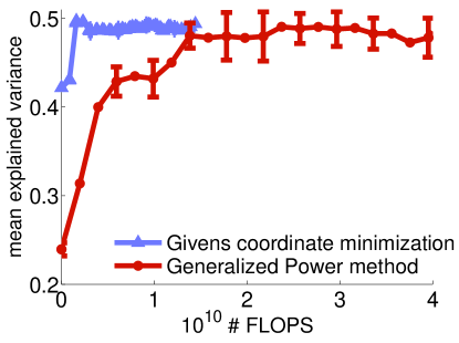
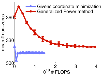
(a) explained variance         (b) number of non-zeros

Figure 1: (a) The explained variance as function of FLOPS of the coordinate minimization method from Algorithm 2 and of the generalized power method by Journée et al. (2010), on a prostate cancer gene expression dataset. (b) The number of non-zeros in the sparse PCA matrix as function of FLOPS of the coordinate minimization method from Algorithm 2 and of the generalized power method by Journée et al. (2010), on a prostate cancer gene expression dataset. The size of the sparse PCA matrix is $12,600\times 102$.

We tested the streaming version of the coordinate descent algorithm for sparse PCA (Algorithm 5, supp. material) on a recent large gene expression data set collected from of six human brains (Hawrylycz et al., 2012). Overall, each of the 20K human genes was measured at 3702 different brain locations, and this data can be used to study the spatial patterns of mRNA expression across the human brain.

We again compared the performance of our approach with that of the Generalized Power Method of Journée et al. (2010).

We split the data into 5 train/test partitions, with each train set including 2962 examples and each test set including 740 examples. We evaluated the amount of variance explained by the model on the test set. We use the adjusted variance procedure suggested in this case by Zou et al. (2006), which takes into account the fact that the sparse principal components are not orthogonal.

For the Generalized Power Method we use the greedy $l_{1}$ version of Journée et al. (2010), with the parameter $\mu$ set to 1. We found the greedy version to be more stable and to be able to produce sparse solutions when the number of components was $m>1$. We used values of $\gamma$ ranging from $0.01$ to $0.2$, and two stopping conditions: “convergence”, where the algorithm was run until its objective converged within a relative tolerance level of $10^{-4}$, and “early stop” where we stopped the algorithm after 14% of the iterations required for convergence.

For our algorithm we used the same range of $\gamma$ values, and used an “early stop” condition where the algorithm was stopped after using 14% of the samples.

Figure 2 demonstrates the tradeoff between floating point operations and explained variance for sparse PCA with 3, 5 and 10 components and with 3 sparsity levels: 5%, 10% and 20%. Using low dimensions is often useful for visual exploration of the data. Each dot represents one instance of the algorithm that was run with a certain value of $\gamma$ and stopping criterion. To avoid clutter we only show instances which performed best in terms of explained variance or few FLOPS.

When strong sparsity is required (5% or 10% sparsity), the givens-rotation coordinate descent algorithm finds solutions faster (blue rectangles are more to the left in Figure 2), and these solutions are similar or better in terms of explained variance.

For low-dimensional less sparse solutions (20% sparsity) we find that the generalized power method finds comparable or better solutions using the same computational cost, but only when the number of components is small, as seen in Figure 2.c,f,i.

(a) max. sparsity 5%          (d) max. sparsity 5%          (g) max. sparsity 5%

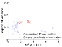
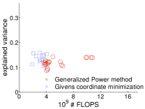
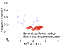
(b) max. sparsity 10%          (e) max. sparsity 10%          (h) max. sparsity 10%

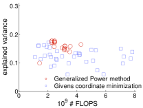
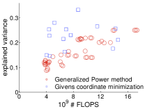
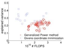
(c) max. sparsity 20%          (f) max. sparsity 20%          (i) max. sparsity 20%

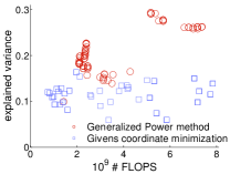
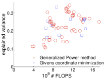
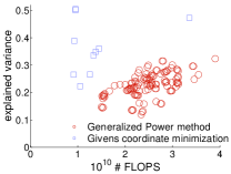
3 components                    5 components                    10 components

Figure 2: The tradeoff between explained variance and computational cost for 3, 5 and 10-component sparse-PCA models applied to Human gene expression data. The models are constrained for maximum sparsity of 5% (a), (d) & (f), 10% (b), (e) & (h) and 20% (c), (f) & (i). Red circles are instances of the Generalized Power method Journée et al. (2010); Blue squares represent the Givens coordinate descent procedure. Both algorithms were run with $\gamma$ in the range [0.01,…,0.2] and two stopping criteria (’early-stop’ and ’convergence’). The points presented are chosen for best performance in terms of computational cost or explained variance. Explained variance was adjusted following Zou et al. (2006)

5 Orthogonal tensor decomposition

Recently it has been shown that many classic machine learning problem such as Gaussian Mixture Models and Latent Dirichlet Allocation can be solved efficiently by using 3rd order moments (Anandkumar et al., 2012a; Hsu & Kakade, 2013; Anandkumar et al., 2012b, c; Chaganty & Liang, 2013). These methods ultimately rely on finding an orthogonal decomposition of 3-way tensors $T\in\mathbb{R}^{d\times d\times d}$, and reconstructing the solution from the decomposition. In this section, we show that the problem of finding an orthogonal decomposition for a tensor $T\in\mathbb{R}^{d\times d\times d}$ can be naturally cast as a problem of optimization over the orthogonal matrix manifold. We then apply Algorithm (1) to this problem, and compare its performance on a task of finding a Gaussian Mixture Model with a state-of-the-art tensor decomposition method, namely the robust Tensor Power Method (Anandkumar et al., 2012a). We find that the Givens coordinate minimization method consistently finds better solutions when the number of mixture components is large.

5.1 Orthogonal tensor decomposition

The problem of tensor decomposition is very hard in general (Kolda & Bader, 2009). However, a certain class of tensors known as “orthogonally decomposable” tensors are easier to decompose, as has been demonstrated recently by Anandkumar et al. (2012a); Hsu & Kakade (2013) and others. In this section, we introduce the problem of orthogonal tensor decomposition, and provide a new characterization of the solution to the tensor-decomposition problem as the solution of an optimization problem on the orthogonal matrix manifold.

The resulting algorithm is similar to one recently proposed by Ishteva et al. (2013). However, we aim for full diagonalization, while they focus on finding a good low-rank approximation. This results in different objective functions: ours involves third-order polynomials on $\mathcal{O}_{d}$, while Ishteva et al.’s results in sixth-order polynomials on the low-rank compact Stiefel manifold. Diagonalizing the tensor $T$ is attainable in our case thanks to the strong assumption that it is orthogonally decomposable. Nonetheless, both methods are extensions of Jacobi’s eigenvalue algorithm to the tensor case, in different setups.

We start with preliminary notations and definitions. We focus here on symmetric tensors $T\in\mathds{R}^{d\times d\times d}$. A third-order tensor is symmetric if its values are identical for any permutation $\sigma$ of the indices: with $T_{i_{1}i_{2}i_{3}}=T_{i_{\sigma(1)}i_{\sigma(2)}i_{\sigma(3)}}$.

We also view a tensor $T$ as a trilinear map.
$T:\mathbb{R}^{d}\times\mathbb{R}^{d}\times\mathbb{R}^{d}\rightarrow\mathbb{R}$: $T(v_{1},v_{2},v_{3})=\sum_{a,b,c=1}^{d}T_{abc}v_{1a}v_{2b}v_{3c}$.

Finally, we also use the three-form tensor product of a vector $u\in\mathbb{R}^{d}$ with itself: $u\otimes u\otimes u\in\mathbb{R}^{d\times d\times d}$, $(u\otimes u\otimes u)_{abc}=u_{a}\cdot u_{b}\cdot u_{c}$. Such a tensor is called a rank-one tensor.

Let $T\in\mathbb{R}^{d\times d\times d}$ be a symmetric tensor.

Definition 4.

A tensor $T$ is orthogonally decomposable if there exists an orthonormal set of vectors $v_{1},\ldots v_{d}\in\mathbb{R}^{d}$, and positive scalars $\lambda_{1},\ldots\lambda_{d}>0$ such that:

$$T=\sum_{i=1}^{d}\lambda_{i}(v_{i}\otimes v_{i}\otimes v_{i}).$$ (7)

Unlike matrices, most symmetric tensors are not orthogonally decomposable. However, as shown by Anandkumar et al. (2012a); Hsu & Kakade (2013); Anandkumar et al. (2013), several problems of interest, notably Gaussian Mixture Models and Latent Dirichlet Allocation do give rise to third-order moments which are orthogonally decomposable in the limit of infinite data.

The goal of orthogonal tensor decomposition is, given an orthogonally decomposable tensor $T$, to find the orthogonal vector set $v_{1},\ldots v_{d}\in\mathbb{R}^{d}$ and the scalars $\lambda_{1},\ldots\lambda_{d}>0$.

We now show that finding an orthogonal decomposition can be stated as an optimization problem over $\mathcal{O}_{d}$:

Theorem 3.

Let $T\in R^{d\times d\times d}$ have an orthogonal decomposition as in Definition 4, and consider the optimization problem

$$\underset{U\in\mathcal{O}_{d}}{\operatorname{max}}f(U)=\sum_{i=1}^{d}T(u_{i},u_{i},u_{i}),$$ (8)

where $U=[u_{1}\,u_{2}\,\ldots\,u_{d}]$. The stable stationary points of the problem are exactly orthogonal matrices $U$ such that $u_{i}=v_{\pi(i)}$ for a permutation $\pi$ on $[d]$. The maximum value they attain is $\sum_{i=1}^{d}\lambda_{i}$.

The proof is given in the supplemental material.

5.2 Coordinate minimization algorithm for orthogonal tensor decomposition

We now adapt Algorithm (1) for solving the problem of orthogonal tensor decomposition of a tensor $T$, by minimizing the objective function 8, $f(U)=-\sum_{i=1}^{d}T(u_{i},u_{i},u_{i})$. For this we need to calculate the form of the function $f\left(U\cdot G(i,j,\theta)\right)$. Define $\tilde{u}_{i}=cos(\theta)u_{i}+sin(\theta)u_{j}$ and $\tilde{u}_{j}=cos(\theta)u_{j}-sin(\theta)u_{i}$.

$$f\left(U\cdot G(i,j,\theta)\right)=\sum_{k\neq i,j}^{d}T(u_{k},u_{k},u_{k})+$$

$$T\left(\tilde{u}_{i},\;\tilde{u}_{i},\;\tilde{u}_{i}\right)+T\left(\tilde{u}_{j},\;\tilde{u}_{j},\;\tilde{u}_{j}\right).$$

Define:

$$g_{t}^{ij}(\theta)=f\left(U\cdot G(i,j,\theta)\right),$$ (9)

and denote by $\tilde{T}$ the tensor such that:

$$\tilde{T}_{ijk}=T(u_{i},u_{j},u_{k}).$$ (10)

Collecting terms, using the symmetry of $T$ and some basic trigonometric identities, we then have:

$$g_{t}^{ij}(\theta)= cos^{3}(\theta)\left(\tilde{T}_{iii}+\tilde{T}_{jjj}-3\tilde{T}_{ijj}-3\tilde{T}_{jii}\right)$$ (11)

$$+ sin^{3}(\theta)\left(\tilde{T}_{iii}-\tilde{T}_{jjj}-3\tilde{T}_{ijj}+3\tilde{T}_{jii}\right)$$

$$+ cos(\theta)\left(3\tilde{T}_{ijj}+3\tilde{T}_{jii}\right)$$

$$+ sin(\theta)\left(3\tilde{T}_{ijj}-3\tilde{T}_{jii}\right).$$

In each step of the algorithm, we maximize $g_{t}^{ij}(\theta)$ over $-\pi\leq\theta<\pi$. The function $g_{t}^{ij}$ has at most 3 maxima that can be obtained in closed form solution, and thus $g_{t}^{ij}$ can be maximized in constant time.

Algorithm 3 Riemannian coordinate maximization for orthogonal tensor decomposition

0:  Symmetric tensor $T\in\mathds{R}^{d\times d\times d}$, initial matrix $U_{0}\in\mathcal{O}_{d}$

  $t=0$

  while not converged do

     1. Sample uniformly at random a pair $(i(t),j(t))$ such that $1\leq i(t)<j(t)\leq d$.

     2. Calculate $\tilde{T}_{iii}$, $\tilde{T}_{jjj}$, $\tilde{T}_{ijj}$, $\tilde{T}_{jii}$ as in 10.

     3. $\theta_{t}=\underset{\theta}{\operatorname{argmax}}\;g_{t}^{ij}(\theta)$, where $g_{t}^{ij}$ is defined as in 11.

     4. $U_{t+1}=U_{t}G(i,j,\theta_{t})$.

     5. $t=t+1$.

  end while

The most computationally intensive part of Algorithm 3 is line 2, naively requiring $O(d^{3})$ operations. This can be improved to $O(d^{2})$ per iteration, with a one-time precomputation of $O(d^{4})$ operations, by maintaining an auxiliary tensor in memory. The more efficient algorithm is not described due to space constraints. We will make the code available online.

5.3 Experiments

Hsu & Kakade (2013) and Anandkumar et al. (2012a) have recently shown how the task of fitting a Gaussian Mixture Model (GMM) with common spherical covariance can be reduced to the task of orthogonally decomposing a third moment tensor. We evaluate the Givens coordinate minimization algorithm using this task. We compare with a state of the art tensor decomposition method, the robust tensor power method, as given in Anandkumar et al. (2012a).

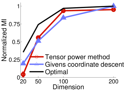
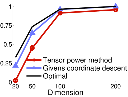
(a) 10,000 samples            (b) 200,000 samples

Figure 3: Clustering performance in terms of normalized MI of the Givens coordinate algorithm vs. the tensor power method of Anandkumar et al. (2012a). Clustering by fitting a GMM from samples drawn from a 20-component GMM with varying dimension, using 3rd order moments. The reconstruction is performed from (a) 10K samples and (b) 200K samples. Blue line with circles marks the Givens coordinate minimization method. Red line with triangles marks the tensor power method, and the black line is the optimal performance if all the GMM parameters are known.

We generated GMMs with the following parameters: number of dimensions in $\{10,\,20,\,50,\,100,\,200\}$, number of samples sampled from the model in $\{10K,30K,50K,100K,200K\}$. We used $20$ components, each with a spherical variance of $2$. The centers were sampled from a Gaussian distribution with an inverse-Wishart distributed covariance matrix. Given the samples, we then constructed the third order moment, decomposed it, and reconstructed the model following the procedure outlined in Anandkumar et al. (2012a). We then clustered the samples according to the reconstructed model, and measured the normalized mutual information (NMI) (Manning et al., 2008) between the learned clustering and the true clusters.

Figure 3 compares the performance of the two methods with the optimal NMI across dimensions. The coordinate minimization method outperforms the tensor power method for the large sample size (200K), whereas for small sample size (10K) the tensor power method performs better for the intermediate dimensions. In Figure 4 we see the performance of both algorithms across all sample sizes for dimension $=100$. We see that the coordinate minimization method again performs better for larger sample sizes. We observed this phenomenon for 50 components as well, and for mixture models with larger variance.

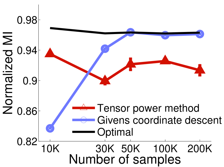
Figure 4: Same task as Figure 3, but for fixed dimension $d=100$ and varying number of samples.

6 Conclusion

We described a framework to efficiently optimize differentiable functions over the manifold of orthogonal matrices. The approach is based on Givens rotations, which we show can be viewed as the parallel of coordinate updates in Euclidean spaces. We prove the procedure’s convergence to a local optimum.

Using this framework, we developed algorithms for two unsupervised learning problems. First, finding sparse principal components; and second, learning a Gaussian mixture model through orthogonal tensor decomposition.

We expect that the framework can be further extended to other problems requiring learning over orthogonal matrices including ICA. Moreover, coordinate descent approaches have some inherent advantages and are sometimes better amenable to parallelization. Developing distributed Givens-rotation algorithms would be an interesting future research direction.

Appendix A Proofs of theorems of section 3

Below we use a slightly modified definition of Algorithm 1. The difference lies only in the sampling procedure, and is essentially a technical difference to ensure that each coordinate step indeed improves the objective or lies at an optimum, so that the proofs could be stated more succinctly.

0:  Differentiable objective function $f$, initial matrix $U_{0}\in\mathcal{O}_{d}$

  $t=0$

  while not converged do

     1. Sample coordinate pairs $(i(t),j(t))$ such that $1\leq i(t)<j(t)\leq d$ uniformly at random without replacement, until the objective function can improve

     2. $U_{t+1}=\underset{\theta}{\operatorname{argmin}}\;f\left(U_{t}\cdot G(i,j,\theta)\right)$.

     3. $t=t+1$.

  end while

Algorithm 4 Riemannian coordinate minimization on $\mathcal{O}_{d}$, sampling variant

Definition 5.

A point $U_{*}\in\mathcal{O}_{d}$ is asymptotically stable with respect to Algorithm 4 if it has a neighborhood $\mathcal{V}$ of $U_{*}$ such that all sequences generated by Algorithm 4 with starting point $U_{0}\in\mathcal{V}$ converge to $U_{*}$.

• Convergence to local optimum
  (1) The sequence of iterates $U_{t}$ of Algorithm 4 satisfies: $\lim_{t\to\infty}||\nabla f(U_{t})||=0$. This means that the accumulation points of the sequence $\{U_{t}\}_{t=1}^{\infty}$ are critical points of $f$.
  (2) Assume the critical points of $f$ are isolated. Let $U_{*}$ be a critical point of $f$. Then $U_{*}$ is a local minimum of $f$ if and only if it is asymptotically stable with regard to the sequence generated by Algorithm 4.

Proof.

(1) Algorithm 4 is obtained by taking a step in each iteration $t$ in the direction of the tangent vector $Z_{t}$, such that for the coordinates $(i(t),j(t))$ we have $(Z_{t})_{ij}=-(\nabla f(U_{t}))_{ij}$, $(Z_{t})_{ji}=-(\nabla f(U_{t}))_{ji}$ , and $(Z_{t})_{kl}=0$ for all other coordinates $(k,l)$.

The sequence of tangent vectors $Z_{t}\in T_{U_{t}}\mathcal{O}_{d}$ is easily seen to be gradient related: $\limsup{k\rightarrow\infty}\langle\nabla f(U_{t}),Z_{t}\rangle<0$ . This follows from $Z_{t}$ being equal to exactly two coordinates of $\nabla f(U_{t})$, with all other coordinates being 0.

Using the optimal step size as we do assures at least as large an increase $f(U_{t})-f(U_{t+1})$ as using the Armijo step size rule (Armijo, 1966; Bertsekas, 1999). Using the fact that the manifold $\mathcal{O}_{d}$ is compact, we obtain by theorem 4.3.1 and corrolary 4.3.2 of Absil et al. (2009) that $\lim_{t\to\infty}||\nabla f(U_{t})||=0$

(2) Since Algorithm 4 produces a monotonically decreasing sequence $f(U_{t})$, and since the manifold $\mathcal{O}_{d}$ is compact, we are in the conditions of Theorems 4.4.1 and 4.4.2 of Absil et al. (2009). These imply that the only critical points which are local minima are asymptotically stable.

∎

We now provide a rate of convergence proof. This proof is a Riemannian version of the proof for the rate of convergence of Euclidean random coordinate descent for non-convex functions given by Patrascu & Necoara (2013).

Definition 6.

For an iterate $t$ of Algorithm 4, and a set of indices $(i(t),j(t))$, we define the auxiliary single variable function $g_{t}^{ij}$ :

$$g_{t}^{ij}(\theta)=f\left(U_{t}\cdot G(i,j,\theta)\right),$$ (12)

Note that $g_{t}^{ij}$ are differentiable and periodic with a period of $2\pi$. Since $\mathcal{O}_{d}$ is compact and $f$ is differentiable there exists a single Lipschitz constant $L(f)>0$ for all $g_{t}^{ij}$.

• Rate of convergence
  Let $f$ be a continuous function with $L$-Lipschitz directional derivatives . Let $U_{t}$ be the sequence generated by Algorithm 4. For the sequence of Riemannian gradients $\nabla f(U_{t})\in T_{U_{t}}\mathcal{O}_{d}$ we have:

  $$\underset{0\leq t\leq T}{\operatorname{max}}E\left[||\nabla f(U_{t})||_{2}^{2}\right]\leq\frac{L\cdot d^{2}\left(f(U_{0})-f_{min}\right)}{T+1}\quad.$$ (13)

Lemma 1.

Let $g:\mathbb{R}\rightarrow\mathbb{R}$ be a periodic differentiable function, with period $2\pi$, and $L-$Lipschitz derivative $g^{\prime}$. Then there for all $\theta\in[-\pi\;\pi]$: $g(\theta)\leq g(0)+\theta g^{\prime}(0)+\frac{L}{2}\theta^{2}$.

Proof.

We have for all $\theta$,
$|g^{\prime}(\theta)-g^{\prime}(0)|\leq L|\theta|$. We now have: $g(\theta)-g(0)-\theta g^{\prime}(0)=\int_{0}^{\theta}g^{\prime}(\tau)-g^{\prime}(0)d\tau\leq\int_{0}^{\theta}|g^{\prime}(\tau)-g^{\prime}(0)|d\tau\leq\int_{0}^{\theta}L|\tau|d\tau=\frac{L}{2}\theta^{2}$. ∎

Corollary 1.

Let $g=g_{i(t+1)j(t+1)}^{t+1}$. Under the conditions of Algorithm 4, we have:
$f(U_{t})-f(U_{t+1})\geq\frac{1}{2L}\nabla_{ij}f(U_{t})^{2}$ for the same constant $L$ defined in 1.

Proof.

By the definition of $g$ we have $f(U_{t+1})=\underset{\theta}{\operatorname{min}}\;g(\theta)$, and we also have $g(0)=f(U_{t})$. Finally, by Eq. 1 of the main paper we have $\nabla_{ij}f(U_{t})=g^{\prime}(0)$. From Lemma 1, we have $g(\theta)-g(0)\leq\theta g^{\prime}(0)+\frac{L}{2}\theta^{2}$. Minimizing the right-hand side with respect to $\theta$, we see that $\underset{\theta}{\operatorname{min}}\;\{g(0)-g(\theta)\}\geq\frac{1}{2L}(g^{\prime}(0))^{2}$. Substituting $f(U_{t+1})=\underset{\theta}{\operatorname{min}}\;g(\theta)$ ,$f(U_{t})=g(0)$, and $\frac{1}{2L}\nabla_{ij}f(U_{t})=g^{\prime}(0)$ completes the result. ∎

Proof of Theorem A.

By Corollary 1, we have $f(U_{t})-f(U_{t+1})\geq\frac{1}{2L}\nabla_{ij}f(U_{t})^{2}$. Recall that $\pm\nabla_{ij}f(U_{t})$ is the $(i,j)$ and $(j,i)$ entry of $\nabla f(U_{t})$. If we take the expectation of both sides with respect to a uniform random choice of indices $i,j$ such that $1\leq i<j\leq d$, we have:

$$E\left[f(U_{t})-f(U_{t+1})\right]\geq\frac{1}{L\cdot d^{2})}||\nabla f(U_{t})||^{2},$$ (14)

Summing the left-hand side gives a telescopic sum which can be bounded by $f(U_{0})-\underset{U\in\mathcal{O}_{d}}{\operatorname{min}}f(U)=f(U_{0})-f_{min}$. Summing the right-hand side and using this bound, we obtain

$$\sum_{t=0}^{T}E\left[||\nabla f(U_{t})||_{2}^{2}\right]\leq L\cdot d^{2}(f(U_{0})-f_{min})$$ (15)

This means that $\underset{0\leq t\leq T}{\operatorname{min}}E\left[||\nabla f(U_{t})||_{2}^{2}\right]\leq\frac{L\cdot d^{2}(f(U_{0})-f_{min})}{T+1}$. ∎

Appendix B Proofs of theorems of section 5

• A tensor $T$ is orthogonally decomposable if there exists an orthonormal set of vectors $v_{1},\ldots v_{d}\in\mathbb{R}^{d}$, and positive scalars $\lambda_{1},\ldots\lambda_{d}>0$ such that:

  $$T=\sum_{i=1}^{d}\lambda_{i}(v_{i}\otimes v_{i}\otimes v_{i}).$$ (16)

• Let $T\in R^{d\times d\times d}$ have an orthogonal decomposition as in Definition 4, and consider the optimization problem

  $$\underset{U\in\mathcal{O}_{d}}{\operatorname{max}}f(U)=\sum_{i=1}^{d}T(u_{i},u_{i},u_{i}),$$ (17)

  where $U=[u_{1}\,u_{2}\,\ldots\,u_{d}]$. The stable stationary points of the problem are exactly orthogonal matrices $U$ such that $u_{i}=v_{\pi(i)}$ for a permutation $\pi$ on $[d]$. The maximum value they attain is $\sum_{i=1}^{d}\lambda_{i}$.

Proof.

For a tensor $T^{\prime}$ denote $\textrm{vec}(T^{\prime})\in\mathbb{R}^{d^{3}}$ the vectorization of $T^{\prime}$ using some fixed order of indices. Set $\hat{T}(U)=\sum_{i=1}^{d}(u_{i}\otimes u_{i}\otimes u_{i})$, with $\hat{T}(U)_{abc}=\sum_{i=1}^{d}u_{ia}u_{ib}u_{ic}$. The sum of trilinear forms in Eq. 17 is equivalent to the inner product in $\mathbb{R}^{d^{3}}$ between $\hat{T}(U)$ and $T$: $\sum_{i=1}^{d}T(u_{i},u_{i},u_{i})=\sum_{i=1}^{d}\sum_{abc}T_{abc}u_{ia}u_{ib}u_{ic}=\sum_{abc}T_{abc}\left(\sum_{i=1}^{d}u_{ia}u_{ib}u_{ic}\right)=\sum_{abc}T_{abc}\hat{T}(U)_{abc}=\textrm{vec}(T)\bm{\cdot}\textrm{vec}(\hat{T}(U))$. Consider the following two facts:
(1)  $\hat{T}(U)_{abc}\leq 1\;\forall a,b,c=1\ldots d$: since the vectors $u_{i}$ are orthogonal, all their components $u_{ia}\leq 1$. Thus $\hat{T}(U)_{abc}=\sum_{i=1}^{d}u_{ia}u_{ib}u_{ic}\leq\sum_{i=1}^{d}u_{ia}u_{ib}=\leq 1$, where the last inequality is because the sum is the inner product of two rows of an orthogonal matrix.
(2)  $||\textrm{vec}(\hat{T}(U))||_{2}^{2}=d$. This is easily checked by forming out the sum of squares explicitly, using the orthonormality of the rows and columns of the matrix $U$.
Assume without loss of generality that $V=I_{d}$. This is because we may replace the terms $T(u_{i},u_{i},u_{i})$ in the objective with $T(V^{T}u_{i},V^{T}u_{i},V^{T}u_{i})$, and because the manifold $V^{T}\mathcal{O}_{d}$ is identical to $\mathcal{O}_{d}$. Thus we have that $T$ is a diagonal tensor, with $T_{aaa}=\lambda_{a}>0$, $a=1\ldots d$. Considering facts (1) and (2) above, we have the following inequality:

$$\underset{U\in\mathcal{O}_{d}}{\operatorname{max}}\sum_{i=1}^{d}T(u_{i},u_{i},u_{i})=\underset{U\in\mathcal{O}_{d}}{\operatorname{max}}\textrm{vec}(\hat{T}(U))\bm{\cdot}T\leq$$ (18)

$$\underset{\hat{T}}{\operatorname{max}}\;\textrm{vec}(\hat{T})\bm{\cdot}T\quad s.t.\quad||\textrm{vec}(\hat{T})||_{\infty}\leq 1\,\wedge\,||\textrm{vec}(\hat{T})||_{2}^{2}=d.$$ (19)

$T$ is diagonal by assumption, with exactly $d$ non-zero entires. Thus the maximum of (16) is attained if and only if $\hat{T}_{aaa}=1$, $a=1\ldots d$, and all other entries of $\hat{T}$ are $0$. The value at the maximum is then $\sum_{i=1}^{d}\lambda_{i}$.

The diagonal ones tensor $\hat{T}$ can be decomposed into $\sum_{i=1}^{d}e_{i}\otimes e_{i}\otimes e_{i}$. Interestingly, in the tensor case, unlike in the matrix case, the decomposition of orthogonal tensors is unique upto permutation of the factors (Kruskal, 1977; Kolda & Bader, 2009). Thus, the only solutions which attain the maximum of 18 are those where $u_{i}=e_{\pi(i)}$, $i=1,\ldots d$. ∎

Appendix C Algorithm for streaming sparse PCA

Following are the details for the streaming sparse PCA version of our algorithm used in the experiments of section 4. The algorithm starts with running the original coordinate minimization procedure on the first $m$ samples. It then chooses the column with the least $l_{2}$ and replaces it with a new data sample, and then reoptimizes on the new set of samples. There is no need for it to converge in the inner iterations, and in practice we found that order $m$ steps after each new sample are enough for good results.

0:  Data stream $a_{i}\in\mathbb{R}^{d}$, number of sparse principal components $m$, initial matrix $U_{0}\in\mathcal{O}_{m}$, sparsity parameter $\gamma\geq 0$, number of inner iterations $L$.

  $AU=[a_{1}a_{2}\ldots a_{m}]\cdot U_{0}$ . //$AU$ is of size $d\times m$

  while not stopped do

     for $t=1\ldots L$ do

        1. Sample uniformly at random a pair $(i(t),j(t))$ such that $1\leq i(t)<j(t)\leq m$.

        2. $\theta_{t+1}=\underset{\theta}{\operatorname{argmax}}$ $\sum_{k=1}^{d}([|cos(\theta)(AU)_{ki(t)}+sin(\theta)(AU)_{kj(t)}|-\gamma]_{+}^{2}$ $+[|-sin(\theta)(AU)_{ki(t)}+cos(\theta)(AU)_{kj(t)}|-\gamma]_{+}^{2})$.

        3.$AU=AU\cdot G(i(t),j(t)),\theta_{t+1})$.

     end for

     4. $i_{min}=\underset{i=1\dots m}{\operatorname{argmin}}||(AU)_{:,i}||_{2}$.

     5. Sample new data point $a_{new}$.

     6. $(AU)_{:,i_{min}}=a_{new}$.

  end while

  $Z=solveForZ(AU,\gamma)$ // Algorithm 6 of  Journée et al. (2010).

  $Z\in\mathbb{R}^{d\times m}$

Algorithm 5 Riemannian coordinate minimization for streaming sparse PCA

References

- Absil et al. (2009) Absil, P-A, Mahony, Robert, and Sepulchre, Rodolphe. Optimization algorithms on matrix manifolds. Princeton University Press, 2009.
- Anandkumar et al. (2012a) Anandkumar, Anima, Ge, Rong, Hsu, Daniel, Kakade, Sham M, and Telgarsky, Matus. Tensor decompositions for learning latent variable models. arXiv preprint arXiv:1210.7559, 2012a.
- Anandkumar et al. (2013) Anandkumar, Anima, Ge, Rong, Hsu, Daniel, and Kakade, Sham M. A tensor spectral approach to learning mixed membership community models. arXiv preprint arXiv:1302.2684, 2013.
- Anandkumar et al. (2012b) Anandkumar, Animashree, Foster, Dean P, Hsu, Daniel, Kakade, Sham M, and Liu, Yi-Kai. A spectral algorithm for latent dirichlet allocation. arXiv preprint arXiv:1204.6703, 2012b.
- Anandkumar et al. (2012c) Anandkumar, Animashree, Hsu, Daniel, and Kakade, Sham M. A method of moments for mixture models and hidden markov models. arXiv preprint arXiv:1203.0683, 2012c.
- Armijo (1966) Armijo, Larry. Minimization of functions having lipschitz continuous first partial derivatives. Pacific Journal of mathematics, 16(1):1–3, 1966.
- Bertsekas (1999) Bertsekas, Dimitri P. Nonlinear programming. Athena Scientific, 1999.
- Chaganty & Liang (2013) Chaganty, Arun Tejasvi and Liang, Percy. Spectral experts for estimating mixtures of linear regressions. arXiv preprint arXiv:1306.3729, 2013.
- d’Aspremont et al. (2007) d’Aspremont, Alexandre, El Ghaoui, Laurent, Jordan, Michael I, and Lanckriet, Gert RG. A direct formulation for sparse pca using semidefinite programming. SIAM review, 49(3):434–448, 2007.
- Golub & Van Loan (2012) Golub, Gene H and Van Loan, Charles F. Matrix computations, volume 3. JHUP, 2012.
- Hawrylycz et al. (2012) Hawrylycz, Michael J, Lein, S, Guillozet-Bongaarts, Angela L, Shen, Elaine H, Ng, Lydia, Miller, Jeremy A, van de Lagemaat, Louie N, Smith, Kimberly A, Ebbert, Amanda, Riley, Zackery L, et al. An anatomically comprehensive atlas of the adult human brain transcriptome. Nature, 489(7416):391–399, 2012.
- Hsu & Kakade (2013) Hsu, Daniel and Kakade, Sham M. Learning mixtures of spherical gaussians: moment methods and spectral decompositions. In Proceedings of the 4th conference on Innovations in Theoretical Computer Science, pp. 11–20. ACM, 2013.
- Ishteva et al. (2013) Ishteva, Mariya, Absil, P-A, and Van Dooren, Paul. Jacobi algorithm for the best low multilinear rank approximation of symmetric tensors. SIAM Journal on Matrix Analysis and Applications, 34(2):651–672, 2013.
- Journée et al. (2010) Journée, Michel, Nesterov, Yurii, Richtárik, Peter, and Sepulchre, Rodolphe. Generalized power method for sparse principal component analysis. The Journal of Machine Learning Research, 11:517–553, 2010.
- Kolda & Bader (2009) Kolda, Tamara G and Bader, Brett W. Tensor decompositions and applications. SIAM review, 51(3):455–500, 2009.
- Kruskal (1977) Kruskal, Joseph B. Three-way arrays: rank and uniqueness of trilinear decompositions, with application to arithmetic complexity and statistics. Linear Algebra and its Applications, 18(2):95 – 138, 1977. ISSN 0024-3795. doi: 10.1016/0024-3795(77)90069-6.
- Manning et al. (2008) Manning, Christopher D, Raghavan, Prabhakar, and Schütze, Hinrich. Introduction to information retrieval, volume 1. Cambridge University Press Cambridge, 2008.
- Nemirovski (1999) Nemirovski, A. Optmization II Numerical Methods for Nonlinear Continuous Optimization. 1999.
- Nesterov (2012) Nesterov, Yu. Efficiency of coordinate descent methods on huge-scale optimization problems. SIAM Journal on Optimization, 22(2):341–362, 2012.
- Patrascu & Necoara (2013) Patrascu, Andrei and Necoara, Ion. Efficient random coordinate descent algorithms for large-scale structured nonconvex optimization. arXiv preprint arXiv:1305.4027, 2013.
- Richtárik & Takáč (2012) Richtárik, Peter and Takáč, Martin. Iteration complexity of randomized block-coordinate descent methods for minimizing a composite function. Mathematical Programming, pp. 1–38, 2012.
- Singh et al. (2002) Singh, Dinesh, Febbo, Phillip G, Ross, Kenneth, Jackson, Donald G, Manola, Judith, Ladd, Christine, Tamayo, Pablo, Renshaw, Andrew A, D’Amico, Anthony V, Richie, Jerome P, et al. Gene expression correlates of clinical prostate cancer behavior. Cancer cell, 1(2):203–209, 2002.
- Zhang & Ghaoui (2012) Zhang, Youwei and Ghaoui, Laurent El. Large-scale sparse principal component analysis with application to text data. arXiv preprint arXiv:1210.7054, 2012.
- Zhang et al. (2012) Zhang, Youwei, d Aspremont, Alexandre, and El Ghaoui, Laurent. Sparse pca: Convex relaxations, algorithms and applications. In Handbook on Semidefinite, Conic and Polynomial Optimization, pp. 915–940. Springer, 2012.
- Zou et al. (2006) Zou, Hui, Hastie, Trevor, and Tibshirani, Robert. Sparse principal component analysis. Journal of computational and graphical statistics, 15(2):265–286, 2006.