Prospects for GeV-TeV detection of
short gamma-ray bursts with extended emission

Abstract

We discuss the GeV to TeV photon emission of gamma-ray bursts (GRBs) within the refreshed shock and the continuous injection scenarios, motivated by the observation of extended emission in a substantial fraction of short GRBs. In the first model we assume that the central engine emits promptly material with a range of Lorentz factors. When the fastest shell starts to decelerate, it drives a forward shock into the ambient medium and a reverse shock in the ejecta. These shocks are reenergized by the slower and later arriving material. In the second model we assume that there is a continued ejection of material over an extended time, and the continuously arriving new material keeps reenergizing the shocks formed by the preceding shells of ejecta. We calculate the synchrotron and synchrotron self-Compton radiation components for the forward and reverse shocks and find that prospective and current GeV to TeV range instruments such as CTA, HAWC, VERITAS , MAGIC and HESS have a good chance to detect afterglows of short bursts with extended emission, assuming a reasonable response time.

1. Introduction

Lightcurves of GRBs at GeV energies are becoming more numerous (Ackermann et al., 2013) thanks to the observations of the Large Area Telescope aboard the Fermi satellite (Atwood et al., 2009). While most of the lightcurves at GeV are for long GRBs, a fraction of short bursts also have a GeV component (e.g. GRB 081024B Abdo et al. (2010) and GRB 090510 De Pasquale et al. (2009)).

The highest energy LAT photons associated with GRBs have $\sim 100\hbox{~{}GeV}$ energy in the comoving frame (Atwood et al., 2013). VERITAS observed the location of 16 Swift detected bursts above $\sim 200\hbox{~{}GeV}$ and found no associated emission (Acciari et al., 2011).

One of the important results of the Swift era (Gehrels et al., 2004) is the discovery of extended emission following some of the short bursts (Gehrels et al., 2006; Norris & Bonnell, 2006). Bostancı et al. (2013) found extended emission following short GRBs in the BATSE data. An extended tail of the prompt emission may be one of the tell-tale signs of a merger event (Zhang et al., 2009). The detection of such extended prompt emission in a high fraction of short bursts prompts us to discuss the effects of a continued energy injection into the afterglow external shock, and to discuss its effects on the high energy lightcurves. The effects of such late-arriving ejecta into the external shocks, whether due to early ejection of a range of Lorentz factors or a continued outflow, are especially important for the detectability with future TeV range observatories, as it flattens the lightcurves providing a higher flux at late times than in the standard impulsive, single Lorentz factor case.

Compact binary merger events are the most promising candidates for gravitational wave detection with the LIGO and VIRGO instruments (e.g. Abadie et al., 2012). The working hypothesis for the short GRB origin is currently the binary merger scenario (e.g. Lee & Ramirez-Ruiz, 2007; Nakar, 2007; Littenberg et al., 2013). Electromagnetic counterpart observations are very important for localization of the gravitational wave source (LIGO Scientific Collaboration et al., 2013), for additional follow up (e.g. Evans et al., 2012) and for constraining the physical nature of the gravitational wave signals. Furthermore, short bursts by themselves are of significant interest for TeV range detections, since their spectra are generally harder then those of long bursts.

Previous theoretical analyses typically considered synchrotron or synchrotron self-Compton (SSC) emission components from top-hat like energy injection episodes when addressing the high energy lightcurves (Dermer et al., 2000; Granot & Sari, 2002; Panaitescu, 2005; Fan & Piran, 2006; Fan et al., 2008; Kumar & Barniol Duran, 2009, 2010; He et al., 2009).

In this paper we discuss the physical processes associated with the refreshed shock and continued ejection scenarios in short GRBs, and we calculate the expected lightcurves in different energy bands. We present illustrative cases, and discuss the observational prospects for GeV and TeV range observatories already in operation or in preparation.

2. Model for GeV and higher energy radiation from refreshed shocks

The basic idea of refreshed shocks is that the central engine ejects material with a distribution of Lorentz factors (LFs) (Rees & Mészáros, 1998). This happens on a short timescale and it can be considered instantaneous. The blob with the highest LF starts decelerating first by accumulating interstellar matter. Forward and reverse shocks form. The trailing part of the emitted blobs will catch up with the decelerated material reenergizing the shocks. This will result in a longer lasting emission by the reverse shock than the usual crossing time (the latter being valid in the case without these refreshed shocks).

The effect of the refreshed shocks is a flattening of the afterglow lightcurve (Sari & Mészáros, 2000). This mechanism is considered a leading candidate for the X-ray plateau (or shallow decay) phase (Nousek et al., 2006; Grupe et al., 2013).

We consider the adiabatic evolution of the blast wave (Mészáros & Rees, 1997) and derive the relation between the LF and radius from energy conservation. At early times the afterglow may be in the radiative regime (Mészáros et al., 1998). In this case the conservation of momentum will yield the correct relation between $R$ or $\Gamma$ and $t$. $R$ and $\Gamma$ are linked by the $R\propto t\Gamma^{2}$ relation (e.g. Mészáros & Rees, 1997; Waxman, 1997).

In our model of refreshed shocks, we assume that a total energy $E_{\rm t}=10^{53}\hbox{~{}erg}~{}E_{\rm t,53}$ is released on a short timescale in a flow, having a power law energy distribution with LF: $E(>\Gamma)=E_{M}(\Gamma/\Gamma_{M})^{-s+1}$, from a minimum ($\Gamma_{m}$) up to a maximum LF ($\Gamma_{M}$). The relation between the total injected energy and the energy imparted to the material with the highest LF ($E_{M}$) is

$$E_{\rm t}=E(>\Gamma_{m})=E_{M}(\Gamma_{m}/\Gamma_{M})^{-s+1}.$$ (1)

Once we set the total energy injected by the central engine and the two limiting LFs, the initial energy ($E_{M}$) can be calculated for a given $s$. It is also possible to fix the extremal LFs and the initial energy (e.g. from observations) and consequently the total injected energy can be determined. A reasonable lower limit of injection LF ($\Gamma_{m}$) is a few tens (Panaitescu et al., 1998) and reasonable values for $\Gamma_{M}$ are a few hundreds.

We introduce the $g$ parameter to describe the density profile of the circumburst environment, $n(R)\propto R^{-g}$ (Mészáros et al., 1998). The usual cases of homogeneous interstellar medium and wind density profile are $g=0$ and $g=2$. The bulk of our illustrative examples are for $g=0$.

The characteristic energy corresponding to material with $\Gamma_{M}$ is $E_{M}$. We will determine physical parameters based on the these quantities at the deceleration radius as reference values for the time evolving quantities. As an example, for $s=2$, the deceleration radius in an interstellar medium of $n=1~{}n_{0}\hbox{~{}cm}^{-3}$ number density is: $R_{M}=(3E_{M}/8\pi nm_{p}c^{2}\Gamma_{M}^{2})^{1/3}=4.6\times 10^{16}\hbox{~{}cm}~{}E_{t,54}^{1/3}n_{0}^{-1/3}\Gamma_{M,2.5}^{-1}(\Gamma_{m}/40)^{1/3}$ and the corresponding timescale $t_{M}=R_{M}/2\Gamma_{M}^{2}c=15{\hbox{~{}s}}~{}E_{t,54}^{1/3}n_{0}^{-1/3}\Gamma_{M,2.5}^{-3}(\Gamma_{m}/40)^{1/3}$. Here we have used Equation 1 to derive the $E_{t}$ dependencies.

The evolution of the physical quantities results from energy conservation (Sari & Mészáros, 2000) in the adiabatic case:

$$R = R_{M}(t/t_{M})^{(s+1)/(7+s-2g)}$$ (2)

$$\Gamma = \Gamma_{M}(t/t_{M})^{-(3-g)/(7+s-2g)}$$ (3)

We do not address the radiative case here, but mention, that it can be accounted for by introducing an additional term in the power law index in the above expressions (Mészáros et al., 1998). The number density of the ejecta, when the reverse shock has crossed (which is approximately at the deceleration radius) is: $n_{b}=E_{M}/4\pi R_{M}^{2}m_{p}c^{3}\Gamma_{M}^{2}T=1.1\times 10^{6}\hbox{~{}cm}^{-3}~{}E_{t,54}^{1/3}\Gamma_{M,2/5}^{-1}(\Gamma_{m}/40)^{1/3}n_{0}^{2/3}T_{0}$, evaluated also for $s=2$, where $T$ is the duration of the burst. The magnetic field will be, as usually assumed, some fraction $\epsilon_{B}$ of the total energy: $B=(32\pi nm_{p}c^{2}\epsilon_{B}\Gamma_{M}^{2})^{1/2}\approx 12.3~{}{\rm G}~{}n_{0}^{1/2}\Gamma_{M,2.5}\epsilon_{B,-2}^{1/2}$. For simplicity, we use the same value for $\epsilon_{B}$ across the forward and reverse shock.

The magnetic field will vary in time as: $B\propto t^{-(6+sg-g)/2(7+s-2g)}$. The reverse shock optical scattering depth at the reference time is: $\tau_{\rm RS}=(\sigma_{T}N)/(4\pi R_{M}^{2})=(\sigma_{T}E_{M})/(4\pi R_{M}^{2}m_{p}c^{2}\Gamma_{M})$. The time dependence results from the change of individual components: $\tau_{\rm RS}\propto t^{-(2-s+sg)/(7-2g+s)}$. The optical depth of the forward shock region is $\tau_{\rm FS}=\sigma_{T}N_{e}/4\pi R^{2}\propto R^{3}R^{-g}/R^{2}\propto t^{(1+s)(1-g)/(7-2g+s)}$. The cooling random LF is defined by an electron whose synchrotron loss timescale is of the order of the dynamical timescale: $\gamma_{c,f}\propto(\Gamma B^{2}t)^{-1}\propto t^{(2-s+gs)/(7-2g+s)}$. The forward shock electrons’ injection LF is: $\gamma_{m,f}\propto\Gamma\propto t^{(2-s+gs)/(7-2g+s)}$. The corresponding synchrotron frequencies: $\varepsilon_{m,f}\propto\Gamma\gamma^{2}_{m,f}B\propto t^{-(24-7g+gs)/(2(7-2g+s))}$.

Synchrotron component - Initially the forward shock will be in the fast cooling regime. The injection electron LF is: $\gamma_{m}=\Gamma\epsilon_{e}m_{p}(p-2)/(p-1)m_{e}$, while the cooling LF is $\gamma_{c}=6\pi m_{e}c/{(1+Y)}\sigma_{T}\Gamma_{M}B^{2}t$, where Y is the Compton parameter (Sari & Esin, 2001). The corresponding synchrotron energies will be $\varepsilon_{m,c}^{\rm syn}=\Gamma\gamma_{m,c}^{2}hq_{e}B/2\pi m_{e}c$, where the $m$ and $c$ indices mark the injection and cooling cases respectively. The spectral shape will be broken power law segments with breaks at these energies. The peak flux of the synchrotron results from considering the individual synchrotron power of the shocked electrons: $F_{\varepsilon,{\rm peak}}^{\rm syn}=({4\pi nR^{3}/3})(m_{e}c^{2}\sigma_{T}\Gamma B/3q_{e})/(4\pi D_{L}^{2})$. The maximum synchrotron energy is derived from the condition that the electron acceleration time is the same order as the radiation timescale, $\varepsilon_{\rm MAX,syn}\approx 2.5\hbox{~{}GeV}(\Gamma_{M}/100)$ (de Jager et al., 1996).

The reverse shock electrons cool at the same rate as the forward shock electrons and their cooling LF ($\gamma_{c}$) will be the same. Their injection LF however is lower by a factor of $\Gamma$, due to the larger density in the ejecta. The reverse shock cooling frequency will be the same as the forward shock, while the injection frequency is lower by $\Gamma^{2}$. The peak of the reverse shock flux is larger by a factor of $\Gamma$.

Synchrotron self-Compton component - Synchrotron photons emitted by the forward and reverse shock electrons will act as seed photons for inverse Compton scattering on their parent electrons. Inverse Compton radiation is expected to occur both in the forward and in the reverse shock (Sari & Esin, 2001). For the SSC spectral shape we consider a simplified approximation, neglecting the logarithmic terms which induce a curvature in the spectrum (Sari & Esin, 2001; Gao et al., 2012). The SSC components will have breaks at $\varepsilon_{m,c}^{\rm SSC}\approx 2\gamma_{m,c}^{2}\varepsilon_{m,c}^{\rm syn}$. The SSC peak flux $F_{F,R}^{\rm SSC}\approx\tau_{F,R}F_{F,R}^{\rm syn}$ for the forward (F) and the reverse (R) shocks respectively.

Other components - There can be an inverse Compton upscattering between the RS electrons and the FS photons, FS electrons and RS photons. We estimated the peaks of these components and found them to be subdominant for the parameters presented here.

Effects suppressing the  TeV radiation -

• Klein-Nishina suppression - At high energies the inverse Compton component can be affected by Klein-Nishina effects. These occur above $\varepsilon\approx\Gamma\gamma m_{e}c^{2}$ and cause a steepening in the spectrum (Guetta & Granot, 2003; Nakar et al., 2009; Wang et al., 2011).

• Pair absorption effects in the source- In the external shock region, the optical depth to $\gamma\gamma\rightarrow e^{\pm}$ process is negligible for most of the parameter space. This is mostly due to the low flux at TeV energies and large radiating volumes resulting in low compactness parameters (Panaitescu et al., 2013).

• Pair suppression on the extragalactic background light (EBL) - To account for the effects of the pair creation with UV to infrared photons of the extragalactic background light we use the model of Finke et al. (2010). This suppression is relevant generally above $100\hbox{~{}GeV}$, but depends significantly on the source redshift. As an example, the lightcurve at $1\hbox{~{}TeV}$ is suppressed by a factor of $\sim 1/3$ for a source at $z=0.1$.

Regarding the last point: the pairs created by TeV range source photons can upscatter the cosmic microwave background (CMB) photons to GeV energies (Plaga, 1995). This would result in a GeV range excess in the spectrum. To account for this component, detailed numerical treatment is needed (see e.g. Dermer et al., 2011) which is not the scope of this work. By neglecting this component, we assume the intergalactic magnetic field (IGMF) is strong enough to change the direction of the pairs by roughly the beam size of the observing instrument (e.g. few $\times 0.1^{\circ}$ for Fermi around $1\hbox{~{}GeV}$). The deflection angle is $\Delta\theta\approx(R_{\rm cool}/R_{\rm Larmor})(\lambda_{\gamma}/D)$ where the expression consists of the cooling length of pairs on the CMB photons, the Larmor radius of the pairs, the mean free path of TeV photons on the EBL, and the source distance in this order. For a source at $z=0.2$ the mean free path of a TeV photon is of the order of a few $\times 100$ Mpc, with uncertainties depending on the EBL model. Assuming the coherence length of the IGMF larger than the cooling length of the pairs, for the magnetic field we get $B>6\times 10^{-16}\hbox{~{}G}(\varepsilon_{\rm source}/{\hbox{~{}TeV}})^{2}$.

On the other hand, such a magnetic field will result in an exceedingly long time delay for the arrival of the GeV photons. Any magnetic field value in excess of $\sim 8\times 10^{-20}\hbox{~{}G}$ will give a delay longer than $10^{5}{\hbox{~{}s}}$, making the association of the excess GeV flux with the GRB difficult.

3. Continued Injection Models

Late energy injection in the forward shock can also occur if there is a prolonged central engine activity following the energy injection episode responsible for the prompt emission (Blandford & McKee, 1976; Dai & Lu, 1998; Zhang & Mészáros, 2001). While in the case of short bursts, in a binary neutron star coalescence scenario the disrupted material is accreted on timescales of $10{\rm ms}$ (Lee & Ramirez-Ruiz, 2007), it is possible that the merger results in the formation of a magnetar, which injects energy on a longer scale. The magnetar injects energy as it spins down, but it can occur also for a black hole central engine. An initial instantaneous energy injection can also be incorporated, which dominates the initial behavior. At sufficiently late times (of the order of one to a few times the deceleration time), the effect of the continuous injection dominates over the initial injection episode. Using the energy conservation and setting an power law injection profile, we can derive dynamic quantities in a similar fashion to Sari & Mészáros (2000), Zhang & Mészáros (2001) or Section 2.

The conservation of the total energy $E_{t}$ at sufficiently late times (Zhang & Mészáros, 2001) reads

$$E_{t}=\frac{L_{0}t}{\kappa+q+1}\left(\frac{t}{t_{0}}\right)^{q}+E_{\rm inst.}\left(\frac{t}{t_{0}}\right)^{-\kappa},$$ (4)

where $q$ is power law temporal index for the injected luminosity and $\kappa$ governs the impulsive energy input ($E_{\rm inst.}$) at early times. $t_{0}$ marks the start of the self similar phase and $\kappa+q+1>0$ has to be fulfilled.

4. Lightcurve Calculations

4.1. Refreshed shock model lightcurves

For the refreshed shocks we adopt a set of realistic nominal parameters, which are: $\Gamma_{m}/40=\Gamma_{M}/300=E_{t,53}=s/3=n_{-1}=\epsilon_{e,-0.5}=\epsilon_{B,-2}=p/2.5=z/0.2=1$, and $g=0$. Unless stated otherwise, we use these parameters in the rest of the article. Here, $\epsilon_{e}$ is the fraction of the energy carried by electrons, $p$ is the exponent in the power law distribution of the shocked electrons, and $z$ is the source redshift. The lightcurves are initially dominated by the forward shock synchrotron emission. Generally, characteristic break frequencies will decrease in time. Initially, the GeV range is above the injection synchrotron frequency and the electrons are in the fast cooling regime. The slope is expected to be $-(-4-4s+g+sg+p/2(24-7g+sg))/2(7+s-2g)=-0.7$ (see Sari & Mészáros (2000) and Figure 1 (bottom) at early times). After $\sim 10^{2}{\hbox{~{}s}}$, or the order of the deceleration time, the forward shock SSC emission starts to dominate the flux. The GeV range is initially (while $t<10^{3}{\hbox{~{}s}}$) below the cooling and characteristic SSC frequencies. The SSC lightcurve has a break when $\varepsilon_{\rm c,SSC}$ passes from above and reaches its peak after $\varepsilon_{\rm m,SSC}$ passes. By this time this is the dominating component by one order of magnitude. The emergence of the SSC component results in a plateau, then a decay with $(-4+8s-36(p-1)/2+(4-8s)/2)/(14+2s)=-0.85$ temporal index, calculated for the $\varepsilon_{\rm obs}>\varepsilon_{\rm m,SSC},\varepsilon_{\rm c,SSC}$ case. The illustrative cases in the figures show a sharp break when some characteristic frequency sweeps through the observing window. In reality we expect a more gradual transition (Granot & Sari, 2002).

Temporal indices for a given ordering of $\varepsilon_{\rm obs},\varepsilon_{\rm m,SSC}$ and $\varepsilon_{\rm c,SSC}$ for one of the components can be found by considering the instantaneous synchrotron (or SSC) spectrum with spectral indices of $\{1/3,-1/2$ or $-(p-1)/2,-p/2\}$ with increasing energy for fast or slow cooling respectively. Thus, for example, the reverse shock SSC with $\varepsilon_{m}^{\rm RSSSC}<\varepsilon_{\rm obs}<\varepsilon_{m}^{\rm RSSSC}$ will have a flux: $F_{\varepsilon}(t)=F^{\rm RSSSC}_{\varepsilon,{\rm peak}}(\varepsilon_{\rm obs}/\varepsilon_{m}^{\rm RSSSC})^{-(p-1)/2}\propto t^{-(18-3g-12s+7gs+p(30-6g-12s+8gs))/6(7+s-2g)}=t^{0.55}$.

The temporal slope of the overall lightcurve will depend on the slope of the dominating component(s). Similarly to Wang et al. (2001), we also find that with certain parameters, the RSSSC can dominate the lightcurve at early times.

Figure 1.— Lightcurves showing individual components for $s=1$ and $s=3$ cases above $1\hbox{~{}GeV}$. The horizontal arrow marks the duration of the fast cooling in the forward shock, the vertical arrow marks the deceleration time of the fastest shell. The lighter shades of the curves indicate flux values prior to the deceleration time, where the Lorentz factor is constant. The shaded region marks an optimistic observation window with Cherenkov telescopes. The notation: FS is short for forward shock, RS for reverse shock, and SSC is synchrotron self-Compton.

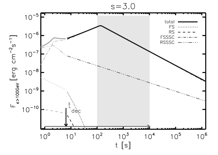
Figure 2.— Lightcurve at $100\hbox{~{}GeV}$. Notations are the same as on figure 1.

4.2. Effect of changing microphysical parameters

Cases with density from $10^{-2}$ to $10\hbox{~{}cm}^{-3}$ have essentially the same lightcurves at late times in both presented cases (see Figure 4 presenting the flux above $100\hbox{~{}GeV}$). Lower values of the density results in fainter fluxes. There is no significant effect on the peak time of the lightcurve (or the end of the plateau phase in the no injection case) happening around $\sim 100{\hbox{~{}s}}$ after the burst.

The effect of changing magnetic parameter $\epsilon_{B}$ has a more accentuated effect. When other parameters remain unchanged the $\epsilon_{B}\approx 10^{-3}$ gives the largest flux both in the injection and the no-injection cases (see Figure 5 Both lower and higher values generally give a lower flux. The peak time of the lightcurve correlates with the value of $\epsilon_{B}$: for lower $\epsilon_{B}$ the peak is earlier.

The lightcurves of afterglows arising from the refreshed shock scenario are shown for three different energy ranges. The first plot is for the range above $1\hbox{~{}GeV}$, since there is abundant data from LAT in this range, allowing a straightforward comparison to past observations (Figure 1). The next plot shows the lightcurves above $100\hbox{~{}GeV}$, which represent a transition between the Fermi and Cherenkov telescope sensitivities for GRBs (Figure 2). The third plot shows the lightcurves above $1\hbox{~{}TeV}$, a so far observationally fallow energy range, but one where the sensitivity of TeV range telescopes is currently being significantly increased, and where CTA and HAWC may bring breakthroughs in the near future (Figure 3).

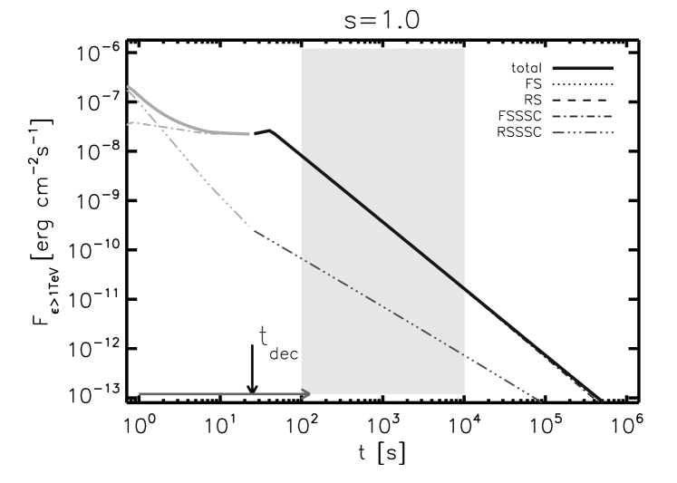
Figure 3.— Lightcurve at $1\hbox{~{}TeV}$. Notations are the same as on figure 1. Note that the synchrotron components are insignificant due to the cutoff at the maximum attainable synchrotron frequency.

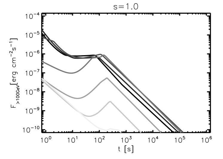
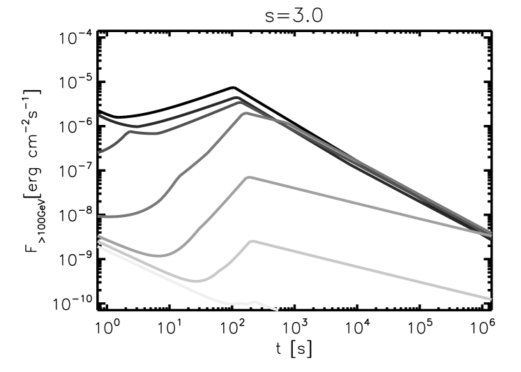
Figure 4.— Lightcurves at $100\hbox{~{}GeV}$ showing the effect of a changing interstellar density. The lightest curve is for $n_{\rm ext}=10^{-5}\hbox{~{}cm}^{-3}$, the darkening shades represent a 10 fold increase, ending at $n_{\rm ext}=10\hbox{~{}cm}^{-3}$. The top figure is for $s=1$, while the bottom figure is for $s=3$.

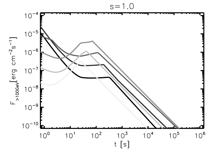
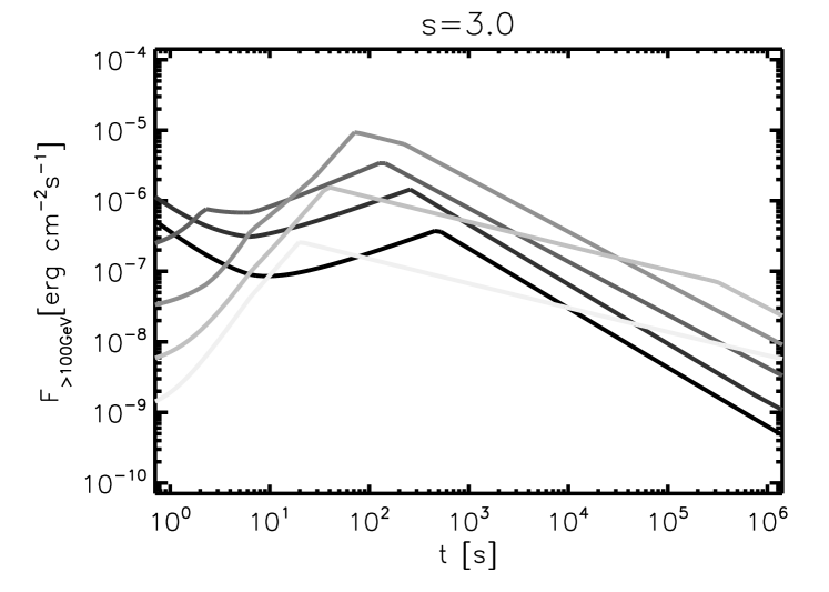
Figure 5.— Lightcurves at $100\hbox{~{}GeV}$ showing the effect of a changing magnetic parameter ($\epsilon_{B}$). The lightest curve is for $\epsilon_{B}=10^{-5}$, the darkening shades represent a tenfold increase, ending at $\epsilon_{B}=1$.

	$\varepsilon_{m}^{\rm SSC}$	$\varepsilon_{c}^{\rm SSC}$	$F^{\rm SSC}_{\varepsilon_{\rm peak}}$
F	$-\frac{36-11g+gs}{2(7+s-2g)}$	$-\frac{-4+8s-3g-7gs}{2(7+s-2g)}$	$-\frac{4-8s+g+5gs}{2(7+s-2g)}$
R	$-\frac{12-3g+gs}{2(7+s-2g)}$	$-\frac{-4+8s-3g-7gs}{2(7+s-2g)}$	$-\frac{16-8s-3g+5sg}{2(7+s-2g)}$

Table 1Temporal indices for calculating the self-Compton radiation behavior.

4.3. Flattening and peak of SSC component

Previous studies predicted that an SSC component provides a flattening of the lightcurve (Sari & Esin, 2001; Dermer et al., 2000). The injection scenario makes this flattening more pronounced or even results in an increase of flux. The peak of the SSC components can be found from: $\varepsilon_{\rm obs}=\max\{\varepsilon_{m}^{\rm FSSSC},\varepsilon_{c}^{\rm FSSSC}\}$ for fast cooling of the forward shock.

As an example, at $100\hbox{~{}GeV}$, the peak occurs in the fast cooling regime, thus we can calculate the peak time from $\varepsilon_{\rm obs}=\varepsilon_{m}^{\rm FSSSC}$. Expressing the SSC injection frequency, we get $\varepsilon_{\rm obs}\propto\Gamma^{6}\epsilon_{e}^{4}\epsilon_{B}^{1/2}g(p)^{4}n_{\rm ext}^{1/2}$, where $g(p)=(p-2)/(p-1)$. Taking the observing energy as a constant and keeping in mind that the time dependence is carried by $\Gamma$ from Equation 3 we find the peak time varies as:

$$t_{\rm peak}\propto\epsilon_{e}^{2(7+s)/9}\epsilon_{B}^{(7+s)/36}g(p)^{2(7+s)/9}n_{\rm ext}^{(s-5)/36}.$$ (5)

This is in agreement with the change of the peak with $n_{\rm ext}$ and $\epsilon_{B}$ presented in the previous subsection (figures 4 and 5): $t_{\rm peak}$ has a very weak dependence on $n_{\rm ext}$ while a change of $10^{5}$ in $\epsilon_{B}$ results in a change of $\approx 13$ and $\approx 25$ in the peak time in Figure 5 (for $s=1$ and $s=3$ respectively).

4.4. Continued injection model lightcurves

Figure 6.— Lightcurves in the continued energy injection case at $100\hbox{~{}GeV}$. The $q$ parameter is $q=-1$ (top) and $q=-0.4$ (bottom). Here $t_{c}$ marks the time when the initial injection term is equal to the continuously injected energy. Other notation is similar to Figure 1.

The continuous injection model lightcurves, based on the discussion in §3, are qualitatively similar to those for the refreshed shock cases. For comparison with the refreshed shock scenario, we use the same parameters as in Section 4.1. The parameter $t_{0}$ is the start of the self similar phase. The value of $t_{c}$ in figure 6 is defined as either the time when the two terms are equal on the right hand side of equation 4, or the time $t_{0}$, whichever is larger. This ensures that the lightcurve is in the self-similar phase and dominated by the continuous injection.

The continuous late injection phase can yield reverse shock and SSC components similarly to the case of refreshed shocks. For simple cases we find a one-to-one correspondence between $s$ and $q$, e.g. in the homogeneous ($g=0$) ISM case, $q=2(s-5)/(s+7)$. To illustrate the similarity, we calculated sample lightcurves based on Zhang & Mészáros (2001) (see Figure 6).

5. Prospects for Observational Detection

The next generation Cherenkov telescopes may be advantageous for detecting the electromagnetic counterpart of a gravitational wave event (Bartos et al., 2014). We concentrate on the afterglow detection. Pointing instruments generally require a time delay from the satellite trigger time to the start of the GeV-TeV observations. Observatories with extended sky coverage can in principle detect both the prompt and the afterglow emission, though with a lower sensitivity.

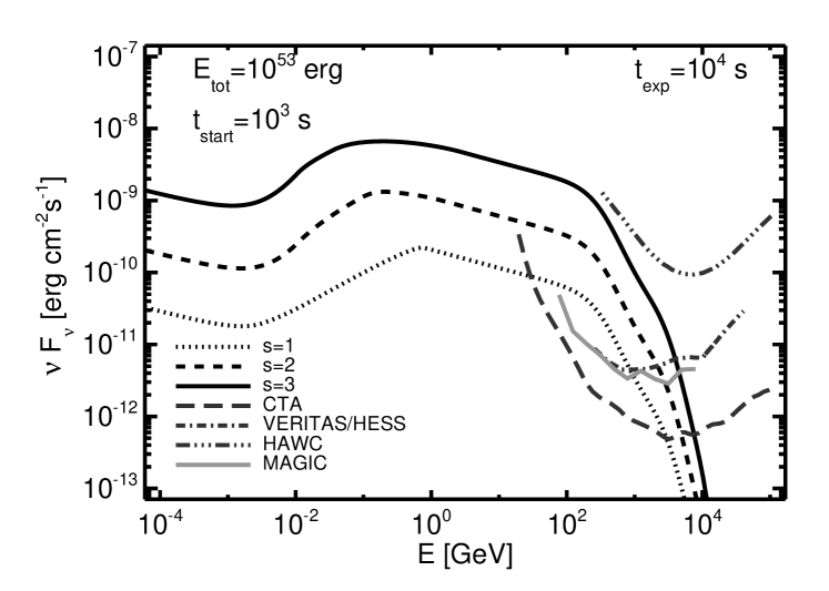
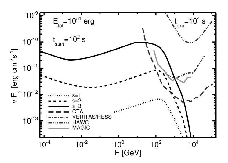
Figure 7.— Average spectrum for the $s=\{1,2,3\}$ cases. The upper panel shows the example case presented in Section 4 for observations starting at $t_{\rm start}=10^{3}{\hbox{~{}s}}$ and lasting for $dt=10^{4}{\hbox{~{}s}}$. The lower figure is a model with total energy of $E_{\rm t}=10^{51}\hbox{~{}erg}$ and $t_{\rm start}=10^{2}{\hbox{~{}s}}$, $dt=10^{4}{\hbox{~{}s}}$. Overlaid are the differential sensitivity curves of CTA, VERITAS/HESS, MAGIC and HAWC.

5.1. Detectability with current and future telescopes

CTA - We calculate the sensitivity of CTA following the treatment of Actis et al. (2011), based on their Fig. 24. The detection capabilities of the future CTA telescope in the context of GRBs was discussed at length by Inoue et al. (2013).

VERITAS and HESS - These instruments have similar sensitivities for our purposes. VERITAS can slew on the order of $100{\hbox{~{}s}}$ to a source with favorable sky position. For a compilation of sensitivity curves see Abeysekara et al. (2013) and references therein, for HESS see Aharonian et al. (2004).

MAGIC - This instrument has the best sensitivity at $\sim 100\hbox{~{}GeV}$ (Aleksić et al., 2012). It has comparable sensitivity to VERITAS/HESS up to $\sim 100\hbox{~{}TeV}$ (see Figure 7). Furthermore, the average slewing time for MAGIC is $\sim 20{\hbox{~{}s}}$ after the alert, which makes it well suited for early follow-up (Garczarczyk et al., 2009).

HAWC - The HAWC instrument is a water Cherenkov observatory with large field of view and duty cycle. It can potentially detect both the prompt and the afterglow emission. Here we take the HAWC sensitivity for steady sources, which is a crude approximation for the long-lasting lightcurves of our models, assuming an observation lasting $10^{4}{\hbox{~{}s}}$ (Abeysekara et al., 2013).

Detection - In general terms, models with energy injection due to either refreshed shocks or continued outflow result in a larger radiation flux at late times than the conventional models. This is evident from Figure 7. The interplay of the brightness and distance of the burst and the slew time of the telescope determines the detection. We assume an average time delay after the satellite trigger time of $t_{start}=10^{3}$ s. In the upper panel the total energy is $E_{t}=10^{53}$ erg and the exposure time is $10^{4}{\hbox{~{}s}}$, while in the lower panel of the figure, we reduced the total energy budget of the GRB to $E_{t}=10^{51}\hbox{~{}erg}$ for the same exposure time. Except for the no-injection (no LF spread, $s=1$) model in the $E_{\rm t}=10^{51}\hbox{~{}erg}$ case, all of the models can be detected at least marginally with CTA and some with VERITAS , MAGIC and HESS. The HAWC instrument can only marginally detect afterglow lightcurves in the most optimistic cases presented here. HAWC is better suited for observing the prompt phase, for which there is a more sensitive data analysis in place, but may be able to detect the very early afterglow.

These figures show that for standard afterglow parameters and average response time, observing GeV-TeV range range radiation from short GRB afterglows is promising with current instruments.

5.2. High energy temporal indices

Both cooling and injection SSC energies are a decreasing functions of time. At $\sim 100\hbox{~{}GeV}$, observations will occur above the highest break frequency and the temporal slope can be calculated from (all SSC parameters):

$$F_{\varepsilon} = F_{\rm peak}(\varepsilon_{c}/\varepsilon_{m})^{-(p-1)/2}(\varepsilon_{\rm obs}/\varepsilon_{c})^{-p/2}$$ (6)

$$\propto t^{-(-32-8s+10g+2gs+p(36-11g+gs))/4(7+s-2g)}.$$ (7)

The slope will be the same irrespective of the cooling regime. This can be compared with measurements, in order to constrain the values of $s$. For example if $g$ and $p$ are known from lower energy observations, the measured high energy slope is very sensitive to the value of $s$. Figure 8 shows an example of slopes for the forward shock SSC at late times for $p=2.5$.

Figure 8.— Contour map of the temporal index as a function of the injection ($s$)- and circumstellar density ($g$) profile (see Equation 7). These are the temporal slopes expected at late times for observing energies $\varepsilon_{\rm obs}>\max\{\varepsilon_{m}^{\rm FSSSC},\varepsilon_{c}^{\rm FSSSC}\}$. Here, $p=2.5$ and possible Klein-Nishina or EBL effects are not taken into account. These would result in a higher $\alpha$.

5.3. X-ray counterparts

As mentioned in the introduction, in the case of gravitational waves, electromagnetic follow-up observations are crucial. That is also the case in the event of a detection of a GRB at TeV energies. Currently the Swift XRT (Burrows et al., 2005) is most likely to provide X-ray follow-up on timescales of $100s$ after the trigger (Evans et al., 2012). Similarly to the GeV-TeV range, we have calculated the lightcurves at $10\hbox{~{}keV}$ (see Figure 9). The X-ray afterglow is dominated by synchrotron radiation. The temporal slope for $s>1$ is visibly shallower than the $s=1$ case, and that is the reason this model is favored for the interpretation of the X-ray plateau. At late times ($10^{5}-10^{6}{\hbox{~{}s}}$), the FSSSC provides a bump in the lightcurve. This late after the trigger only the brighter bursts are detected with XRT, and typically no unambiguous bump is observed (Zhang, 2014).

In contrast to the X-rays, the GeV-TeV range lightcurves are dominated by the SSC from the FS. In the framework of the refreshed shock model, the difference between the temporal slopes can be expressed as (from Sari & Mészáros (2000) and Equation 7): $\Delta\alpha=\alpha_{X}-\alpha_{\rm TeV}=(3-g)(p-2)/(7-g+s)$, where the X-ray has the shallower decay. For e.g. in case of $p=2.5$ the X-ray slope is flatter at most by $\sim 0.2$, where the expression for $\Delta\alpha$ has its maximum, for $s=1$ and $g=0$ (no injection and constant ISM case). In general, $\Delta\alpha\lesssim 3(p-2)/8$.

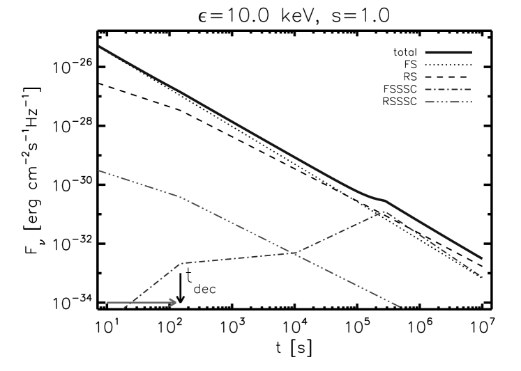
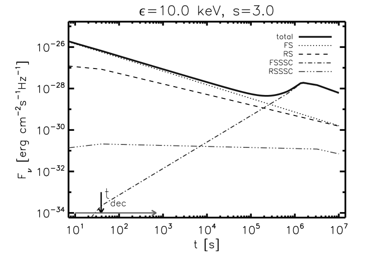
Figure 9.— X-ray lightcurve for an afterglow with standard parameters.

5.4. The case of GRB 090510

The high-energy lightcurve of the archetypical short GRB 090510 is consistent with a single power law. Certainly, up to now there is no definite proof of an SSC component at high energies. The GeV range lightcurves can be explained by one component (see e.g. De Pasquale et al. (2009) or Kouveliotou et al. (2013) for GRB 130427A). As shown in Figure 1, the SSC component starts to dominate at a later time and there is a pronounced ”bump” feature in the lightcurve. This feature becomes more prominent with increasing $s$. There are two possibilities how the SSC could be dominant in the GRB afterglows. In the first case, the whole GeV-range flux is attributed to SSC. This needs fine tuned parameters as the SSC peak needs to be very early. The second option is to have a very smooth transition in time between synchrotron dominated and SSC dominated times. This requires less fine tuning because e.g. the temporal slopes of the two components will not be too different (see section 5.3) but the fluxes have to match within errors. Thus we speculate that a bump feature is present in the lightcurve (see Fig 1. in De Pasquale et al. (2009)), but not significant. This points to a low value of $s$, close to $1$

6. Discussion and Conclusions

Thus far there is a dearth of short GRB afterglow lightcurves observed above  GeV energies, compared to long GRBs. Nonetheless, future and current observatories offer realistic prospects for detecting GeV-TeV range emission from these sources, which are also the prime targets for gravitational wave detectors.

We have calculated the TeV range radiation for the refreshed shock and the continued injection afterglow models of short GRBs. The refreshed shock model involves a range of injected LFs, the slower material catching up at later times, reenergizing the shocks, and qualitatively similar results are obtained in continuous injection models.

Our aim was to show that even though many GeV lightcurves decline rapidly, the sensitivity of current and future TeV range instruments is sufficient to detect short GRB afterglows in the framework of the refreshed shock model, where the decline of the flux can be slower. In the relevant GeV-TeV range we found that the afterglow SSC components are the main contributors to the flux. The usual time dependences for the non-injection cases are recovered by setting $s=1$ and $g=0$ or $g=2$.

We also showed that in the simple case of an ISM environment and adiabatic afterglow, there is a one-to-one correspondence between the continuous injection model and the instantaneous injection refreshed shock model with a range of LFs. A possible distinction between these scenarios can be made by following the X-ray lightcurve. In the continuous injection model the plateau is expected to end abruptly (Zhang, 2013).

We have calculated the dependence of the peak time (peak or plateau in the lightcurve) on the microphysical parameters and found that it correlates positively with the $\epsilon_{e}$, $\epsilon_{e}$ and $g(p)$ parameters, while it anticorrelates with the external density $n_{\rm ext}$. For late times and high energies we have calculated the expected temporal slope. These can be used, when the first TeV range measurements are carried out, to constrain the $s$ index of the LF distribution.

The general behavior of a model with a Lorentz factor spread or late injection is that for the same total energy output it starts out dimmer and has a flatter decline at later times. It has a more pronounced plateau phase for higher $s$ parameter, ending at $\sim 1000{\hbox{~{}s}}$. The importance of the refreshed shock and continuous injection models lie in supplying energy to the external shock complex at late times, flattening the afterglow decay, and thus making it more favorable for detection at TeV energies. The flattening in the lightcurve is most notable at $10^{2}-10^{3}{\hbox{~{}s}}$ after the burst trigger. Our calculations show that current and next generation ground-based instruments will be well suited to detect the GeV-TeV emission of short bursts with extended emission. In the event of a gravitational wave trigger, even if Swift or Fermi are in Earth occultation, the ground-based GeV-TeV detections could provide a good counterpart localization.

We thank NASA NNX13AH50G and OTKA K077795 for partial support, and David Burrows, Charles Dermer, Abe Falcone and Dmitry Zaborov for discussions. We further thank Stefano Covino and Markus Garczarczyk for providing the MAGIC sensitivity curve and the referee for a thorough report.

References

- Abadie et al. (2012) Abadie, J. et al. 2012, ApJ, 760, 12, 1205.2216
- Abdo et al. (2010) Abdo, A. A. et al. 2010, ApJ, 712, 558
- Abeysekara et al. (2013) Abeysekara, A. U. et al. 2013, ArXiv e-prints, 1306.5800
- Acciari et al. (2011) Acciari, V. A. et al. 2011, ApJ, 743, 62, 1109.0050
- Ackermann et al. (2013) Ackermann, M. et al. 2013, ApJS, 209, 11, 1309.4899
- Actis et al. (2011) Actis, M. et al. 2011, Experimental Astronomy, 32, 193, 1008.3703
- Aharonian et al. (2004) Aharonian, F. et al. 2004, ApJ, 614, 897, arXiv:astro-ph/0407118
- Aleksić et al. (2012) Aleksić, J. et al. 2012, Astroparticle Physics, 35, 435, 1108.1477
- Atwood et al. (2009) Atwood, W. B. et al. 2009, ApJ, 697, 1071, 0902.1089
- Atwood et al. (2013) ——. 2013, ApJ, 774, 76, 1307.3037
- Bartos et al. (2014) Bartos, I. et al. 2014, ArXiv e-prints, 1403.6119
- Blandford & McKee (1976) Blandford, R. D., & McKee, C. F. 1976, Physics of Fluids, 19, 1130
- Bostancı et al. (2013) Bostancı, Z. F., Kaneko, Y., & Göğüş, E. 2013, MNRAS, 428, 1623, 1210.2399
- Burrows et al. (2005) Burrows, D. N. et al. 2005, Space Science Reviews, 120, 165, arXiv:astro-ph/0508071
- Dai & Lu (1998) Dai, Z. G., & Lu, T. 1998, A&A, 333, L87, arXiv:astro-ph/9810402
- de Jager et al. (1996) de Jager, O. C., Harding, A. K., Michelson, P. F., Nel, H. I., Nolan, P. L., Sreekumar, P., & Thompson, D. J. 1996, ApJ, 457, 253
- De Pasquale et al. (2009) De Pasquale, M. et al. 2009, ArXiv e-prints, 0910.1629
- Dermer et al. (2011) Dermer, C. D., Cavadini, M., Razzaque, S., Finke, J. D., Chiang, J., & Lott, B. 2011, ApJ, 733, L21, 1011.6660
- Dermer et al. (2000) Dermer, C. D., Chiang, J., & Mitman, K. E. 2000, ApJ, 537, 785
- Evans et al. (2012) Evans, P. A. et al. 2012, ApJS, 203, 28, 1205.1124
- Fan & Piran (2006) Fan, Y., & Piran, T. 2006, MNRAS, 370, L24, arXiv:astro-ph/0601619
- Fan et al. (2008) Fan, Y.-Z., Piran, T., Narayan, R., & Wei, D.-M. 2008, MNRAS, 384, 1483, 0704.2063
- Finke et al. (2010) Finke, J. D., Razzaque, S., & Dermer, C. D. 2010, ApJ, 712, 238, 0905.1115
- Gao et al. (2012) Gao, H., Lei, W.-H., Wu, X.-F., & Zhang, B. 2012, ArXiv e-prints, 1204.1386
- Garczarczyk et al. (2009) Garczarczyk, M. et al. 2009, ArXiv e-prints, 0907.1001
- Gehrels et al. (2004) Gehrels, N. et al. 2004, ApJ, 611, 1005, arXiv:astro-ph/0405233
- Gehrels et al. (2006) ——. 2006, Nature, 444, 1044
- Granot & Sari (2002) Granot, J., & Sari, R. 2002, ApJ, 568, 820, arXiv:astro-ph/0108027
- Grupe et al. (2013) Grupe, D., Nousek, J. A., Veres, P., Zhang, B., & Gehrels, N. 2013, ArXiv e-prints, 1305.3236
- Guetta & Granot (2003) Guetta, D., & Granot, J. 2003, MNRAS, 340, 115, arXiv:astro-ph/0208156
- He et al. (2009) He, H.-N., Wang, X.-Y., Yu, Y.-W., & Mészáros, P. 2009, ApJ, 706, 1152, 0911.4217
- Inoue et al. (2013) Inoue, S. et al. 2013, Astroparticle Physics, 43, 252, 1301.3014
- Kouveliotou et al. (2013) Kouveliotou, C. et al. 2013, ApJ, 779, L1, 1311.5245
- Kumar & Barniol Duran (2009) Kumar, P., & Barniol Duran, R. 2009, MNRAS, 400, L75, 0905.2417
- Kumar & Barniol Duran (2010) ——. 2010, MNRAS, 409, 226, 0910.5726
- Lee & Ramirez-Ruiz (2007) Lee, W. H., & Ramirez-Ruiz, E. 2007, New Journal of Physics, 9, 17, astro-ph/0701874
- LIGO Scientific Collaboration et al. (2013) LIGO Scientific Collaboration et al. 2013, ArXiv e-prints, 1304.0670
- Littenberg et al. (2013) Littenberg, T. B., Coughlin, M., Farr, B., & Farr, W. M. 2013, Phys. Rev. D, 88, 084044, 1307.8195
- Mészáros & Rees (1997) Mészáros, P., & Rees, M. J. 1997, ApJ, 476, 232, arXiv:astro-ph/9606043
- Mészáros et al. (1998) Mészáros, P., Rees, M. J., & Wijers, R. A. M. J. 1998, ApJ, 499, 301, arXiv:astro-ph/9709273
- Nakar (2007) Nakar, E. 2007, Phys. Rep., 442, 166, arXiv:astro-ph/0701748
- Nakar et al. (2009) Nakar, E., Ando, S., & Sari, R. 2009, ApJ, 703, 675, 0903.2557
- Norris & Bonnell (2006) Norris, J. P., & Bonnell, J. T. 2006, ApJ, 643, 266, arXiv:astro-ph/0601190
- Nousek et al. (2006) Nousek, J. A. et al. 2006, ApJ, 642, 389, arXiv:astro-ph/0508332
- Panaitescu (2005) Panaitescu, A. 2005, MNRAS, 363, 1409, arXiv:astro-ph/0508426
- Panaitescu et al. (1998) Panaitescu, A., Meszaros, P., & Rees, M. J. 1998, ApJ, 503, 314, arXiv:astro-ph/9801258
- Panaitescu et al. (2013) Panaitescu, A., Vestrand, W. T., & Wozniak, P. 2013, ArXiv e-prints, 1308.3197
- Plaga (1995) Plaga, R. 1995, Nature, 374, 430
- Rees & Mészáros (1998) Rees, M. J., & Mészáros, P. 1998, ApJ, 496, L1+, arXiv:astro-ph/9712252
- Sari & Esin (2001) Sari, R., & Esin, A. A. 2001, ApJ, 548, 787, arXiv:astro-ph/0005253
- Sari & Mészáros (2000) Sari, R., & Mészáros, P. 2000, ApJ, 535, L33, arXiv:astro-ph/0003406
- Wang et al. (2001) Wang, X. Y., Dai, Z. G., & Lu, T. 2001, ApJ, 546, L33, arXiv:astro-ph/0010320
- Wang et al. (2011) Wang, X.-Y., He, H.-N., & Li, Z. 2011, International Journal of Modern Physics D, 20, 2023
- Waxman (1997) Waxman, E. 1997, ApJ, 491, L19, arXiv:astro-ph/9709190
- Zhang (2013) Zhang, B. 2013, ArXiv e-prints, 1310.4893
- Zhang & Mészáros (2001) Zhang, B., & Mészáros, P. 2001, ApJ, 552, L35, arXiv:astro-ph/0011133
- Zhang et al. (2009) Zhang, B. et al. 2009, ApJ, 703, 1696, 0902.2419
- Zhang (2014) Zhang, B.-B. 2014, in preparation