Explicit estimates for solutions of mixed elliptic problems

Abstract.

We deal with the existence of quantitative estimates for solutions of mixed problems to an elliptic second order equation in divergence form with discontinuous coefficient. Our concern is to estimate the solutions with explicit constants, for domains in $\mathbb{R}^{n}$ ($n\geq 2$) of class $C^{0,1}$. The existence of $L^{\infty}$ and $W^{1,q}$-estimates is assured for $q=2$ and any $q<n/(n-1)$ (depending on the data), whenever the coefficient is only measurable and bounded. The proof method of the quantitative $L^{\infty}$-estimates is based on the DeGiorgi technique developed by Stampacchia. By using the potential theory, we derive $W^{1,p}$-estimates for different ranges of the exponent $p$ depending on that the coefficient is either Dini-continuous or only measurable and bounded. In this process, we establish new existences of Green functions on such domains. The last but not least concern is to unify (whenever possible) the proofs of the estimates to the extreme Dirichlet and Neumann cases of the mixed problem.

1. Introduction

The knowledge of the data makes all the difference on the real world applications of boundary value problems. Quantitative estimates are of extremely importance in any other area of science such as engineering, biology, geology, even physics, to mention a few. In the existence theory to the nonlinear elliptic equations, fixed point arguments play a crucial role. The solution may exist such that belongs to a bounded set of a functional space, where the boundedness constant is frequently given in an abstract way. Their derivation is so complicated that it is difficult to express them, or they include unknown ones that are achieved by a contradiction proof, as for instance the Poincaré constant for nonconvex domains. The majority of works consider the same symbol for any constant that varies from line to line along the whole paper (also known as universal constant). In conclusion, the final constant of the boundedness appears completely unknown from the physical point of view. In presence of this, our first concern is to explicit the dependence on the data of the boundedness constant. To this end, first (Section 3.1) we solve in $H^{1}$ the Dirichlet, mixed and Neumann problems to an elliptic second order equation in divergence form with discontinuous coefficient, and simultaneously we establish the quantitative estimates with explicit constants. Besides in Section 3.2 we derive $W^{1,q}$ ($q<n/(n-1)$) estimative constants involving $L^{1}$ and measure data, via the technique of solutions obtained by limit approximation (SOLA) (cf. [4, 13, 10, 35]).

Dirichlet, Neumann, and mixed problems with respect to uniformly elliptic equation in divergence form is widely investigated in the literature (see [1, 3, 14, 20, 21, 22, 28, 33, 38] and the references therein) when the leading coefficient is a function on the spatial variable, and the boundary values are given by assigned Lebesgue functions. Meanwhile, many results on the regularity for elliptic PDE are appearing [2, 6, 7, 15, 16, 17, 19, 23, 24, 26, 29, 32, 34, 36, 39] (see Section 6 for details). Notwithstanding their estimates seem to be inadequate for physical and technological applications. For this reason, the explicit description of the estimative constants needs to carry out. Since the smoothness of the solution is invalidated by the nonsmoothness of the coefficient and the domain, Section 4 is devoted to the direct derivation of global and local $L^{\infty}$-estimates.

It is known that the information ’The gradient of a quantity belongs to a $L^{p}$ space with $p$ larger than the space dimension’ is extremely useful for the analysis of boundary value problems to nonlinear elliptic equations in divergence form with leading coefficient $a(x,T)=a(x,T(x))\in L^{\infty}(\Omega)$, where $T$ is a known function, usually the temperature function, such as the electrical conductivity in the thermoelectric [9, 8] and thermoelectrochemical [11] problems. It is also known that one cannot expect in general that the integrability exponent for the gradient of the solution of an elliptic equation exceeds a prescribed number $p>2$, as long as arbitrary elliptic $L^{\infty}$-coefficients are admissable [17]. Having this in mind, in Section 6 we derive $W^{1,p}$-estimates of weak solutions, which verify the representation formula, of the Dirichlet, Neumann, and mixed problems to an elliptic second order equation in divergence form. The proof is based on the existence of Green kernels, which are described in Section 5, whenever the coefficients are whether continuous or only measurable and bounded (inspired in some techniques from [25, 31, 27]).

2. Statement of the problem

Let $\Omega$ be a domain (that is, connected open set) in $\mathbb{R}^{n}$ ($n\geq 2$) of class $C^{0,1}$, and bounded. Its boundary $\partial\Omega$ is constituted by two disjoint open $(n-1)$-dimensional sets, $\Gamma_{D}$ and $\Gamma$, such that $\partial\Omega=\bar{\Gamma}_{D}\cup\bar{\Gamma}$. The Dirichlet situation $\Gamma_{D}=\partial\Omega$ (or equivalently $\Gamma=\emptyset$), and the Neumann situation $\Gamma=\partial\Omega$ (or equivalently $\Gamma_{D}=\emptyset$) are available.

Let us consider the following boundary value problem, in the sense of distributions,

(1) $$-\nabla\cdot(a\nabla u)=f-\nabla\cdot{\bf f} \Omega;$$ in

(2) $$(a\nabla u-{\bf f})\cdot{\bf n}=h \Gamma;$$ on

(3) $$u=g \Gamma_{D},$$ on

where $\bf n$ is the unit outward normal to the boundary $\partial\Omega$.

Set for any $q\geq 1$

$$V_{q}=\left\{\begin{array}[]{ll}W^{1,q}_{\Gamma_{D}}(\Omega)=\{v\in W^{1,q}(\Omega):\ v=0\mbox{ on }\Gamma_{D}\}&\mbox{ if }|\Gamma_{D}|>0\\ \left.\begin{array}[]{l}V_{q}(\partial\Omega)=\{v\in W^{1,q}(\Omega):\ \int_{\partial\Omega}v(x)\mathrm{ds}=0\}\\ V_{q}(\Omega)=\{v\in W^{1,q}(\Omega):\ \int_{\Omega}v(x)\mathrm{dx}=0\}\end{array}\right\}&\mbox{ otherwise}\end{array}\right.$$

the Banach space endowed with the seminorm of $W^{1,q}(\Omega)$, taking the Poincaré inequalities (4)-(5) into account, since any bounded Lipschitz domain has the cone property. Here $|\cdot|$ stands for the $(n-1)$-Lebesgue measure. Also $|A|$ stands for the Lebesgue measure of a set $A$ of $\mathbb{R}^{n}$. The significance of $|\cdot|$ depends on the kind of the set.

Defining the $W^{1,q}$-norm by

$$\|v\|_{1,q,\Omega}:={1\over C_{*}+1}(\|v\|_{q,\Omega}+\|\nabla v\|_{q,\Omega}),$$

with $C_{*}$ being anyone of the Poincaré constants

(4) $$\|v--\int_{\Sigma}v\mathrm{ds}\|_{q,\Omega}\leq C_{*}\|\nabla v\|_{q,\Omega}, \forall v\in W^{1,q}(\Omega);$$

(5) $$\|v--\int_{\Omega}v\mathrm{dx}\|_{q,\Omega}\leq C_{*}\|\nabla v\|_{q,\Omega}, \forall v\in W^{1,q}(\Omega),$$

where $\Sigma\subset\partial\Omega$, and $-\int_{A}$ means the integral average over the set $A$ of positive measure, the Sobolev and trace inequalities read

(6) $$\|v\|_{q^{*},\Omega}\leq S_{q}\|\nabla v\|_{q,\Omega};$$

(7) $$\|v\|_{q_{*},\partial\Omega}\leq K_{q}\|\nabla v\|_{q,\Omega}, \quad\forall v\in V_{q}.$$

Hence further we call (6) the Sobolev inequality, and for the general situation the $W^{1,q}$-Sobolev inequality. Analogously, the trace inequality may be stated. For $1\leq q<n$, $q^{*}=qn/(n-q)$ and $q_{*}=q(n-1)/(n-q)$ are the critical Sobolev and trace exponents such that correspond, respectively, to ${W}^{1,q}(\Omega)\hookrightarrow{L}^{q^{*}}(\Omega)$ and $W^{1,q}(\Omega)\hookrightarrow L^{q_{*}}(\partial\Omega)$. For $1<q<n$, the best constants of the Sobolev and trace inequalities are, respectively, (for smooth functions that decay at infinity, see [40] and [5])

$$S_{q} = \pi^{-1/2}n^{-1/q}\left({q-1\over n-q}\right)^{1-1/q}\left[{\Gamma(1+n/2)\Gamma(n)\over\Gamma(n/q)\Gamma(1+n-n/q)}\right]^{1/n};$$

$$K_{q} = \pi^{1-q\over 2}\left({q-1\over n-q}\right)^{q-1}\left[{\Gamma\left({q(n-1)\over 2(q-1)}\right)\Big{/}\Gamma\left({n-1\over 2(q-1)}\right)}\right]^{q-1\over n-1}.$$

We observe that $q^{*}>1$ is arbitrary if $q=n$. Here $\Gamma$ stands for the gamma function. Set by $\omega_{n}$ the volume of the unit ball $B_{1}(0)$ of $\mathbb{R}^{n}$, that is, $\omega_{n}=\pi^{n/2}/\Gamma(n/2+1)$ and $\Gamma(n/2+1)=(n/2)!$ if $n$ is even, and $\Gamma(n/2+1)=\pi^{1/2}2^{-(n+1)/2}n(n-2)(n-4)\cdots 1$ if $n$ is odd. Moreover, the relationship $\sigma_{n-1}=n\omega_{n}$ holds true, where $\sigma_{n-1}=2\pi^{n/2}/\Gamma(n/2)$ denotes the area of the unit sphere $\partial B_{1}(0)$.

For $n>1$, from the fundamental theorem of calculus applied to each of the $n$ variables separately, it follows that

(8) $$\|u\|_{n/(n-1),\Omega}\leq n^{-1/2}\|\nabla u\|_{1,\Omega}.$$

We emphasize that the above explicit constant is not sharp, since there exists the limit constant $S_{1}=\pi^{-1/2}n^{-1}[\Gamma(1+n/2)]^{1/n}$ [40].

Definition 2.1.

We say that $u$ is weak solution to (1)-(3), if it verifies $u=g$ a.e. on $\Gamma_{D}$, and

(9) $$\int_{\Omega}a\nabla u\cdot\nabla v\mathrm{dx}=\int_{\Omega}{\bf f}\cdot\nabla v\mathrm{dx}+\int_{\Omega}fv\mathrm{dx}+\int_{\Gamma}hv\mathrm{ds},\quad\forall v\in V_{2},$$

where $g\in L^{2}(\Gamma_{D})$, ${\bf f}\in{\bf L}^{2}(\Omega)$, $f\in L^{t}(\Omega)$, with $t=(2^{*})^{\prime}$, i.e. $t=2n/(n+2)$ if $n>2$ and any $t>1$ if $n=2$, $h\in L^{s}(\Gamma)$, with $s=2(n-1)/n$ if $n>2$ and any $s>1$ if $n=2$, and $a\in L^{\infty}(\Omega)$ satisfies $0<a_{\#}\leq a\leq a^{\#}$ a.e. in $\Omega$.

Since $\Omega$ is bounded, we have that $\Omega\subset B_{\partial(\Omega)}(x)$, where $\delta(\Omega):={\rm diam}(\Omega)$, for every $x\in\Omega$. We emphasize that the existence of equivalence between the strong (1)-(3) and weak (9) formulations is only available under sufficiently data. For instance, the Green formula may be applied if $a\nabla u\in{\bf L}^{2}(\Omega)$ and $\nabla\cdot(a\nabla u)\in L^{2}(\Omega)$.

3. Some $W^{1,q}$-constants ($q\leq 2$)

The presented results in this Section are valid whether $a$ is a matrix or a function such that obeys the measurable and boundedness properties. We emphasize that in the matrix situation $a\nabla u\cdot\nabla v=a_{ij}\partial_{i}u\partial_{j}v$, under the Einstein summation convention. Here we restrict to the function situation for the sake of simplicity.

3.1. $H^{1}$-solvability

We recall the existence result in the Hilbert space $H^{1}$ in order to express its explicit constants in the following propositions, namely Propositions 3.1 and 3.2 corresponding to the mixed and the Neumann problems, respectively.

Proposition 3.1.

If $|\Gamma_{D}|>0$, then there exists $u\in H^{1}(\Omega)$ being a weak solution to (1)-(3). If $g=0$, then $u$ is unique. Letting $\widetilde{g}\in H^{1}(\Omega)$ as an extension of $g\in L^{2}(\Gamma_{D})$, i.e. it is such that $\widetilde{g}=g$ a.e. on $\Gamma_{D}$, the following estimate holds

$$\|\nabla u\|_{2,\Omega} \leq (a^{\#}/a_{\#}+1)\|\nabla\widetilde{g}\|_{2,\Omega}+$$

$$+ {1\over a_{\#}}\left(\|{\bf f}\|_{2,\Omega}+C_{n}(\|f\|_{t,\Omega},\|h\|_{s,\Gamma})\right),$$

where $C_{n}(A,B)=S_{2}A+K_{2}B$ if $n>2$, $C_{2}(A,B)=|\Omega|^{1/t^{\prime}}S_{2t/(3t-2)}A+|\Omega|^{1/(2s^{\prime})}K_{2s/(2s-1)}B$ if $t<2$, and $C_{2}(A,B)=|\Omega|^{1/t^{\prime}}A/\sqrt{2}+|\Omega|^{1/(2s^{\prime})}\\ K_{2s/(2s-1)}B$ if $t\geq 2$. In particular, $u-\widetilde{g}\in H^{1}_{\Gamma_{D}}(\Omega)$ is unique.

Proof.

For $g\in L^{2}(\Gamma_{D})$ there exists an extension $\widetilde{g}\in H^{1}(\Omega)$ such that $\widetilde{g}=g$ a.e. on $\Gamma_{D}$. The existence and uniqueness of a weak solution $w\in H^{1}_{\Gamma_{D}}(\Omega)$ is well-known via the Lax-Milgram Lemma, to the variational problem

(11) $$\int_{\Omega}a\nabla w\cdot\nabla v\mathrm{dx}=\int_{\Omega}({\bf f}-a\nabla\widetilde{g})\cdot\nabla v\mathrm{dx}+\int_{\Omega}fv\mathrm{dx}+\int_{\Gamma}hv\mathrm{ds},$$

for all $v\in H^{1}_{\Gamma_{D}}(\Omega)$. Therefore, the required solution is given by $u=w+\widetilde{g}$.

If $g=0$, $\widetilde{g}=0$ and then $u\equiv w$.

Taking $v=w\in H^{1}_{\Gamma_{D}}(\Omega)$ as a test function in (11), applying the Hölder inequality, and using the lower and upper bounds of $a$, we obtain

$$a_{\#}\|\nabla w\|_{2,\Omega}^{2}\leq\left(\|{\bf f}\|_{2,\Omega}+a^{\#}\|\nabla\widetilde{g}\|_{2,\Omega}\right)\|\nabla w\|_{2,\Omega}+\|f\|_{t,\Omega}\|w\|_{t^{\prime},\Omega}+\|h\|_{s,\Gamma}\|w\|_{s^{\prime},\Gamma}.$$

For $n>2$, this inequality reads

$$a_{\#}\|\nabla w\|_{2,\Omega}\leq\|{\bf f}\|_{2,\Omega}+a^{\#}\|\nabla\widetilde{g}\|_{2,\Omega}+S_{2}\|f\|_{2n/(2+n),\Omega}+K_{2}\|h\|_{2(n-1)/n,\Gamma},$$

implying (3.1).

Consider the case of dimension $n=2$. For $t,s>1$, using the Hölder inequality in (8) if $t^{\prime}\leq 2$, in (6) if $t^{\prime}>2$, and in (7) for any $s>1$, we have

$$\|w\|_{t^{\prime},\Omega}\leq|\Omega|^{1/t^{\prime}-1/2}\|w\|_{2,\Omega}\leq{1\over\sqrt{2}}|\Omega|^{1/t^{\prime}-1/2}\|\nabla w\|_{1,\Omega}\leq{1\over\sqrt{2}}|\Omega|^{1/t^{\prime}}\|\nabla w\|_{2,\Omega},\quad(t\geq 2);$$

$$\|w\|_{t^{\prime},\Omega}\leq S_{2t/(3t-2)}\|\nabla w\|_{2t/(3t-2),\Omega}\leq S_{2t/(3t-2)}|\Omega|^{1/t^{\prime}}\|\nabla w\|_{2,\Omega},\quad(t<2);$$

$$\|w\|_{s^{\prime},\Gamma}\leq K_{2s/(2s-1)}\|\nabla w\|_{2s/(2s-1),\Omega}\leq K_{2s/(2s-1)}|\Omega|^{1/(2s^{\prime})}\|\nabla w\|_{2,\Omega}.$$

This concludes the proof of Proposition 3.1. ∎

Proposition 3.2 (Neumann).

If $|\Gamma_{D}|=0$, then there exists a unique $u\in V_{2}$ being a weak solution to (1)-(3). Moreover, the following estimate holds

(12) $$\|\nabla u\|_{2,\Omega}\leq{1\over a_{\#}}\left(\|{\bf f}\|_{2,\Omega}+C_{n}(\|f\|_{t,\Omega},\|h\|_{s,\Gamma})\right),$$

where $C_{n}(A,B)$ is given as in Proposition 3.1.

Proof.

The existence and uniqueness of a weak solution $u\in V_{2}$ is consequence of the Lax-Milgram Lemma (see Remark 3.1). The estimate (12) follows the same argument used to prove (3.1). ∎

Remark 3.1.

The meaning of the Neumann solution $u\in V_{2}$ in Proposition 3.2 should be understood as $u\in V_{2}(\partial\Omega)$ solving (9) for all $v\in V_{2}(\partial\Omega)$, or $u\in V_{2}(\Omega)$ solving (9) for all $v\in V_{2}(\Omega)$.

3.2. $W^{1,q}$-solvability ($q\leq n/(n-1)$)

The existence of a solution is recalled in the following proposition in accordance to $L^{1}$-theory, that is via solutions obtained by limit approximation (SOLA) (cf. [4, 13, 10, 35]), in order to determine the explicit constants.

Proposition 3.3.

Let $g=0$ on $\Gamma_{D}$ (possibly empty), ${\bf f}\in{\bf L}^{2}(\Omega)$, $f\in L^{1}(\Omega)$, $h\in L^{1}(\Gamma)$, and $a\in L^{\infty}(\Omega)$ satisfy $0<a_{\#}\leq a\leq a^{\#}$ a.e. in $\Omega$. For any $1\leq q<n/(n-1)$ there exists $u\in V_{q}$ solving (9) for every $v\in V_{q^{\prime}}$. Moreover, we have the following estimate

$$\|\nabla u\|_{q,\Omega} \leq C_{1}(\Omega,n,q)\left({\|{\bf f}\|_{2,\Omega}\over a_{\#}}+\sqrt{\varkappa(\|f\|_{1,\Omega}+\|h\|_{1,\Gamma})\over a_{\#}}\right)$$

$$+C_{2}\left(n,q,{\|{\bf f}\|_{2,\Omega}\over a_{\#}}+\sqrt{\varkappa(\|f\|_{1,\Omega}+\|h\|_{1,\Gamma})\over a_{\#}}\right),$$

with $\varkappa=2$ if $|\Gamma_{D}|>0$, $\varkappa=4$ if $|\Gamma_{D}|=0$, and

$$C_{1}(\Omega,n,q)=|\Omega|^{1/q-1/2}\left\{\begin{array}[]{ll}{(n-q)^{3/2}\over q(n-2)(n+q-nq)^{1/2}}2^{\frac{1}{q}+\frac{3n-q(n+1)}{2(n-q)}}&\mbox{ if }n>2\\ (2-q)^{-1/2}2^{\frac{(6-q)q-2}{2q}}&\mbox{ if }n=2\end{array}\right.$$

$$C_{2}(n,q,A)=\left\{\begin{array}[]{ll}A^{\frac{2(n-q)}{q(n-2)}}\left({n-q\over n+q-nq}\right)^{\frac{n-q}{q(n-2)}}2^{\frac{(2-q)(nq-n+q)}{q^{2}(n-2)}}S_{q}^{\frac{n(2-q)}{q(n-2)}}&\mbox{ if }n>2\\ A^{\frac{2}{q-1}}|\Omega|^{1/q-1/2}{\left[(q-1)(3-q)^{\frac{3-q}{q-1}}\right]^{\frac{2-q}{2q}}\over(2-q)^{1/(q-1)}}2^{\ell}S_{q}^{\frac{3-q}{q-1}}&\mbox{ if }n=2\end{array}\right.$$

where $\ell\in]2,+\infty[$ is explicitly given in (18).

Proof.

For each $m\in\mathbb{N}$, take

$$f_{m}={mf\over m+|f|}\in L^{\infty}(\Omega),\quad h_{m}={mh\over m+|h|}\in L^{\infty}(\Gamma).$$

Applying Propositions 3.1 and 3.2, there exists a unique solution $u_{m}\in V_{2}$ to the following variational problem

(16) $$\int_{\Omega}a\nabla u_{m}\cdot\nabla v\mathrm{dx}=\int_{\Omega}{\bf f}\cdot\nabla v\mathrm{dx}+\int_{\Omega}f_{m}v\mathrm{dx}+\int_{\Gamma}h_{m}v\mathrm{ds},\quad\forall v\in V_{2}.$$

In particular, (16) holds for all $v\in V_{q^{\prime}}$ ($q^{\prime}>n$).

In order to pass to the limit (16) on $m$ $(m\rightarrow\infty)$ let us establish the estimate (3.3) for $\nabla u_{m}$.

Case $|\Gamma_{D}|>0$. From $L^{1}$-data theory (see, for instance, [35]), let us choose

$$v={{\rm sign}(u_{m})}[1-1/(1+|u_{m}|)^{s}]\in W^{1,2}_{\Gamma_{D}}(\Omega)\cap L^{\infty}(\Omega),\quad\mbox{for }s>0,$$

as a test function in (16). Hence it follows that

$$a_{\#}\int_{\Omega}{s|\nabla u_{m}|^{2}\over(1+|u_{m}|)^{s+1}}\mathrm{dx}\leq s\|{\bf f}\|_{2,\Omega}\|{\nabla u_{m}\over(1+|u_{m}|)^{s+1\over 2}}\|_{2,\Omega}+\|f\|_{1,\Omega}+\|h\|_{1,\Gamma},$$

and consequently

$$\int_{\Omega}{|\nabla u_{m}|^{2}\over(1+|u_{m}|)^{s+1}}\mathrm{dx}\leq{1\over(a_{\#})^{2}}\|{\bf f}\|_{2,\Omega}^{2}+{2\over sa_{\#}}(\|f\|_{1,\Omega}+\|h\|_{1,\Gamma}).$$

By the Hölder inequality with exponents $2/q$ and $2/(2-q)>1$, we have

(17) $$\int_{\Omega}|\nabla u_{m}|^{q}\mathrm{dx}\leq\left(\int_{\Omega}\frac{|\nabla u_{m}|^{2}}{(1+|u_{m}|)^{s+1}}\mathrm{dx}\right)^{\frac{q}{2}}\left(\int_{\Omega}(1+|u_{m}|)^{\frac{(s+1)q}{2-q}}\mathrm{dx}\right)^{\frac{2-q}{2}}.$$

Set

$$M(s):={\|{\bf f}\|_{2,\Omega}\over a_{\#}}+\left({2(\|f\|_{1,\Omega}+\|h\|_{1,\Gamma})\over a_{\#}s}\right)^{1/2}.$$

Let us choose $s>0$ such that $(s+1)q/(2-q)=q^{*}=nq/(n-q)$ which is possible since $1\leq q<n/(n-1)$, that is $s=(n+q-nq)/(n-q)$. Then, gathering the above two inequalities, and inserting (6) for $u_{m}\in V_{2}\hookrightarrow V_{q}$ with $(q\leq 2)$, we deduce

$$\|\nabla u_{m}\|_{q,\Omega}\leq M(s)2^{\frac{2-q}{2q}(\frac{nq}{n-q}-1)}\left(|\Omega|^{1/q-1/2}+(S_{q}\|\nabla u_{m}\|_{q,\Omega})^{\frac{n(2-q)}{2(n-q)}}\right)$$

$$\leq M({n+q-nq\over n-q})2^{\frac{2-q}{2q}(\frac{nq}{n-q}-1)}|\Omega|^{1/q-1/2}+{\frac{n(2-q)}{2(n-q)}}\|\nabla u_{m}\|_{q,\Omega}+$$

$$+{\frac{q(n-2)}{2(n-q)}}[M({n+q-nq\over n-q})]^{\frac{2(n-q)}{q(n-2)}}2^{\frac{(2-q)(nq-n+q)}{q^{2}(n-2)}}S_{q}^{\frac{n(2-q)}{q(n-2)}},$$

using the Young inequality $AB\leq\epsilon A^{a}/a+B^{b}/(b\epsilon^{b/a})$, for $A,B\geq 0$, $\epsilon>0$, and $a,b>1$ such that $1/a+1/b=1$, with $\epsilon=1$, and $a=2(n-q)/[n(2-q)]$ if $n>2$.

For $n=2$, $s>0$ is chosen such that $(s+1)q/(2-q)<q^{*}=2q/(2-q)$ which is possible since $1\leq q<2$, that is $s<1$. Using the above Young inequality with $a=2/(s+1)$, we find

$$(1+|u_{m}|)^{(s+1)q/(2-q)}\leq 2^{\frac{(s+1)q}{2-q}-1}(1+|u_{m}|^{(s+1)q/(2-q)})\leq$$

$$\leq 2^{\frac{(s+2)q-2}{2-q}}+{1-s\over 2}\left({s+1\over 2\epsilon}\right)^{(s+1)/(1-s)}2^{\frac{2[(s+2)q-2]}{(2-q)(1-s)}}+\epsilon|u_{m}|^{q^{*}}.$$

Let us choose, for instance, $s=2-q<1$, and $\epsilon=[2S_{q}M(s)]^{-2q/(2-q)}$. Then, we obtain

$$\|\nabla u_{m}\|_{q,\Omega}\leq M(s)\left(\epsilon^{(2-q)/(2q)}S_{q}\|\nabla u_{m}\|_{q,\Omega}+\right.$$

$$\left.+|\Omega|^{1/q-1/2}\left[2^{\frac{(s+2)q-2}{2-q}}+{1-s\over 2}\left({s+1\over 2\epsilon}\right)^{(s+1)/(1-s)}2^{\frac{2[(s+2)q-2]}{(2-q)(1-s)}}\right]^{\frac{2-q}{2q}}\right)$$

$$\leq{\frac{1}{2}}\|\nabla u_{m}\|_{q,\Omega}+M(2-q)|\Omega|^{1/q-1/2}\times\left[2^{\frac{(4-q)q-2}{2q}}+\right.$$

$$\left.+{1\over 2}\left[(q-1)(3-q)^{\frac{3-q}{q-1}}\right]^{\frac{2-q}{2q}}2^{\ell}[M(2-q)]^{\frac{3-q}{q-1}}S_{q}^{\frac{3-q}{q-1}}\right],$$

where $\ell$ is given by

(18) $$\ell=\frac{2[(s+2)q-2]-(2-3q)(s+1)}{2q(1-s)}=\frac{-5q^{2}+19q-10}{2q(q-1)}\rightarrow 2^{+},$$

as $q\rightarrow 2^{-}$. Hence, we find (3.3) with $\varkappa=2$.

Case $|\Gamma_{D}|=0$. We choose, for $s>0$,

$$v=-{{\rm sign}(u_{m})\over(1+|u_{m}|)^{s}}+-\int_{\partial\Omega}{{\rm sign}(u_{m})\over(1+|u_{m}|)^{s}}\mathrm{ds}\in V_{2}(\partial\Omega);$$

$$v=-{{\rm sign}(u_{m})\over(1+|u_{m}|)^{s}}+-\int_{\Omega}{{\rm sign}(u_{m})\over(1+|u_{m}|)^{s}}\mathrm{dx}\in V_{2}(\Omega),$$

as a test function in (16). Since $|v|\leq 2$ a.e. in $\Omega$, it follows that

$$\int_{\Omega}{|\nabla u_{m}|^{2}\over(1+|u_{m}|)^{s+1}}\mathrm{dx}\leq{1\over(a_{\#})^{2}}\|{\bf f}\|_{2,\Omega}^{2}+{4\over sa_{\#}}(\|f\|_{1,\Omega}+\|h\|_{1,\Gamma}).$$

Then, we argue as in the above case, concluding (3.3) with $\varkappa=4$.

For both cases, we can extract a subsequence of $u_{m},$ still denoted by $u_{m},$ such that it weakly converges to $u$ in $W^{1,q}(\Omega)$, where $u\in V_{q}$ solves the limit problem (9) for all $v\in V_{q^{\prime}}$. ∎

Remark 3.2.

In terms of Proposition 3.3, the terms on the right hand side of (9) have sense, since $v\in W^{1,q^{\prime}}(\Omega)\hookrightarrow C(\bar{\Omega})$ for $q^{\prime}>n,$ that is, $q<n/(n-1)$.

Remark 3.3.

The existence of a solution, which is given at Proposition 3.3, is in fact unique for the class of SOLA solutions (cf. [4, 13, 10]). By the uniqueness of solution in the Hilbert space, this unique SOLA solution is the weak solution of $V_{2}$, if the data belong to the convenient $L^{2}$ Hilbert spaces.

Finally, we state the following version of Proposition 3.3, which will be required in Section 5, with datum belonging to the space of all signed measures with finite total variation $\mathcal{M}(\Omega)=\left({C}_{0}(\Omega)\right)^{\prime}$.

Proposition 3.4.

Let $g=0$ on $\Gamma_{D}$ (possibly empty), $a\in L^{\infty}(\Omega)$ satisfy $0<a_{\#}\leq a\leq a^{\#}$ a.e. in $\Omega$, and for each $x\in\Omega$, $\delta_{x}\in\mathcal{M}(\Omega)$ be the Dirac delta function. For any $1\leq q<n/(n-1)$ there exists $u\in V_{q}$ solving

$$\int_{\Omega}a\nabla u\cdot\nabla v\mathrm{dx}=\langle\delta_{x},v\rangle_{\mathcal{M}(\Omega)\times{C}_{0}(\Omega)},\quad\forall v\in C_{0}(\Omega)\cap V_{1},$$

for every $i=1,\cdots,n$. Moreover, we have the following estimate

(19) $$\|\nabla u\|_{q,\Omega}\leq C_{1}(\Omega,n,q)\sqrt{\varkappa/a_{\#}}+C_{2}(n,q,\sqrt{\varkappa/a_{\#}}),$$

where the constants $C_{1}(\Omega,n,q)$, $C_{2}(n,q,A)$, and $\varkappa$ are determined in Proposition 3.3.

Proof.

Since the Dirac delta function $\delta_{x}\in\mathcal{M}(\Omega)$ can be approximated by a sequence $\{f_{m}\}_{m\in\mathbb{N}}\subset L^{\infty}(\Omega)$ such that

$$\|f_{m}\|_{1,\Omega}=1,\quad\mbox{and}\quad\lim_{m\rightarrow\infty}\int_{\Omega}f_{m}\varphi\mathrm{dx}=\langle\delta_{x},\varphi\rangle_{\mathcal{M}(\Omega)\times{C}_{0}(\Omega)},\ \forall\varphi\in{C}_{0}(\Omega),$$

the identity (16) holds, with $f$ replaced by $f_{m}$, ${\bf f}=0$ in $\Omega$, and $h=0$ on $\Gamma$, for all $v\in V_{2}$ and in particular for all $v\in C_{0}(\Omega)\cap V_{1}$. Then, we may proceed by using the argument already used in the proof of Proposition 3.3, with $\|f\|_{1,\Omega}=1$, and $\|{\bf f}\|_{1,\Omega}=\|h\|_{1,\Gamma}=0$, to conclude (19). ∎

4. $L^{\infty}$-constants

In this Section, we establish some maximum principles, by recourse to the De Giorgi technique [38], via the analysis of the decay of the level sets of the solution. We begin by deriving the explicit estimates in the mixed case $|\Gamma_{D}|>0$.

Proposition 4.1.

Let $p>n\geq 2$, $|\Gamma_{D}|>0$, and $u\in H^{1}(\Omega)$ be any weak solution to (1)-(3) in accordance with Definition 2.1. If $g\in L^{\infty}(\Gamma_{D})$, ${\bf f}\in{\bf L}^{p}(\Omega)$, $f\in L^{np/(p+n)}(\Omega)$, and $h\in L^{(n-1)p/n}(\Gamma)$, then we have

(20) $${\rm ess}\sup_{\Omega}|u|\leq{\rm ess}\sup_{\Gamma_{D}}|g|+$$

$$+{C_{n}\over a_{\#}}|\Omega|^{1/n-1/p}\left(\|{\bf f}\|_{p,\Omega}+S_{p^{\prime}}\|f\|_{np/(p+n),\Omega}+K_{p^{\prime}}\|h\|_{(n-1)p/n,\Gamma}\right),$$

where $C_{n}=2^{n(p-2)/[2(p-n)]}S_{2}$ if $n>2$, and $C_{2}=2^{(3p-2)/[2(p-2)]}$.

Proof.

Let $k\geq k_{0}={\rm ess}\sup\{|g(x)|:\ x\in\Gamma_{D}\}$. Choosing $v={\rm sign}(u)(|u|-k)^{+}={\rm sign}(u)\max\{|u|-k,0\}\in H^{1}_{\Gamma_{D}}(\Omega)$ as a test function in (9), then $\nabla v=\nabla u\in{\bf L}^{2}(A(k))$, and we deduce

(21) $$a_{\#}\int_{A(k)}|\nabla u|^{2}\mathrm{dx}\leq\|{\bf f}\|_{2,A(k)}\|\nabla u\|_{2,A(k)}+$$

$$+\|f\|_{{np\over p+n},\Omega}\|(|u|-k)^{+}\|_{{np\over np-n-p},\Omega}+\|h\|_{(n-1)p/n,\Gamma}\|(|u|-k)^{+}\|_{{(n-1)p\over np-n-p},\Gamma},$$

where $A(k)=\{x\in\Omega:\ |u(x)|>k\}$. Using the Hölder inequality, it follows that

$$\|{\bf f}\|_{2,A(k)}\leq\|{\bf f}\|_{p,\Omega}|A(k)|^{1/2-1/p}\qquad(p>2).$$

Making use of (6)-(7) and $(|u|-k)^{+}\in W^{1,q}_{\Gamma_{D}}(\Omega)$ with $q=p^{\prime}<n$, and the Hölder inequality, we get

$$\|(|u|-k)^{+}\|_{np/(n(p-1)-p),\Omega} \leq S_{p^{\prime}}\|\nabla u\|_{2,A(k)}|A(k)|^{1/p^{\prime}-1/2};$$

$$\|(|u|-k)^{+}\|_{(n-1)p/(n(p-1)-p),\Gamma} \leq K_{p^{\prime}}\|\nabla u\|_{2,A(k)}|A(k)|^{1/p^{\prime}-1/2},$$

if provided by $p^{\prime}<2\leq n$. Inserting last three inequalities into (21) we obtain

(22) $$\|\nabla u\|_{2,A(k)}\leq C_{n,p}|A(k)|^{1/2-1/p},$$

where the positive constant $C_{n,p}$ is

$$C_{n,p}=\left(\|{\bf f}\|_{p,\Omega}+S_{p^{\prime}}\|f\|_{np/(p+n),\Omega}+K_{p^{\prime}}\|h\|_{(n-1)p/n,\Gamma}\right)/a_{\#},\quad\forall n\geq 2.$$

Taking into account that $A(h)\subset A(k)$ when $h>k>k_{0}$, we find

(23) $$(h-k)|A(h)|^{1/\alpha}\leq\|(|u|-k)^{+}\|_{\alpha,A(h)}\leq\|(|u|-k)^{+}\|_{\alpha,A(k)}:=I,\quad\forall\alpha\geq 1.$$

Case $n>2$. Take $\alpha=2^{*}=2n/(n-2)$ in (23). Making use of (6) and $(|u|-k)^{+}\in W^{1,q}_{\Gamma_{D}}(\Omega)$ with $q=2$, and inserting (22), we deduce

$$I\leq S_{2}\|\nabla u\|_{2,A(k)}\leq S_{2}C_{n,p}|A(k)|^{1/2-1/p}.$$

Therefore, we conclude

$$|A(h)|\leq\left(S_{2}C_{n,p}\over h-k\right)^{2^{*}}|A(k)|^{\beta},\qquad\beta=2^{*}(1/2-1/p),$$

where $\beta>1$ if and only if $p>n$. By appealing to [38, Lemma 4.1] we obtain

$$|A(k_{0}+S_{2}C_{n,p}|\Omega|^{(\beta-1)/\alpha}2^{\beta/(\beta-1)})|=0.$$

This means that the essential supremmum does not exceed the well determined constant $M:=k_{0}+S_{2}C_{n,p}|\Omega|^{(\beta-1)/\alpha}2^{\beta/(\beta-1)}$.

Case $n=2$. Choose $\alpha=2$ in (23). Using (8) for $(|u|-k)^{+}\in W^{1,2}_{\Gamma_{D}}(\Omega)$ followed by the Hölder inequality, and inserting (22), we obtain

$$I\leq{1\over\sqrt{2}}\|\nabla u\|_{2,A(k)}|A(k)|^{1/2}\leq{C_{2,p}\over\sqrt{2}}|A(k)|^{1-1/p}.$$

Therefore, we find

$$|A(h)|\leq\left(C_{2,p}/\sqrt{2}\over h-k\right)^{2}|A(k)|^{\beta},\qquad\beta=2(1-1/p),$$

where $\beta>1$ if and only if $p>2$. Then, (20) holds by appealing to [38, Lemma 4.1] as in the anterior case ($n>2$).

This completes the proof of Proposition 4.1. ∎

Remark 4.1.

The Dirichlet problem studied by Stampacchia in [38] coincides with (1)-(3), with $\Gamma=\emptyset$, $f=g=0$, and $n>2$.

Let us extend Proposition 4.1 up to the boundary.

Proposition 4.2.

Under the conditions of Proposition 4.1, any weak solution $u\in H^{1}_{\Gamma_{D}}(\Omega)$ to (1)-(3) satisfies, for $p>2(n-1)$ if $n>2$,

(24) $$\qquad{\rm ess}\sup_{\Omega\cup\Gamma}|u|\leq{\rm ess}\sup_{\Gamma_{D}}|g|+{2^{(n-1)(p-2)/[p-2(n-1)]}\over a_{\#}}|\Omega|^{1/[2(n-1)]-1/p}\times$$

$$\times\left[\left(|\Omega|^{(n-2)/[2n(n-1)]}S_{2}+K_{2}\right)\|{\bf f}\|_{p,\Omega}+\right.$$

$$\left.+\left(|\Omega|^{(n-2)/[2n(n-1)]}S_{2}S_{b^{\prime}}+K_{2}S_{p^{\prime}}\right)\|f\|_{np/(p+n),\Omega}+\right.$$

$$\left.+\left(|\Omega|^{(n-2)/[2(n-1)^{2}]}S_{2}K_{b^{\prime}}+K_{2}K_{p^{\prime}}\right)\|h\|_{(n-1)p/n,\Gamma}\right],$$

with $1/b=1/p+(n-2)/[2n(n-1)]$. For $n=2$, $p>2\alpha/(\alpha-1)$, and $\alpha>1$, then any weak solution $u\in H^{1}_{\Gamma_{D}}(\Omega)$ to (1)-(3) satisfies

(25) $${\rm ess}\sup_{\Omega\cup\Gamma}|u|\leq{\rm ess}\sup_{\Gamma_{D}}|g|+{2^{\frac{p(\alpha+1)-2\alpha}{p(\alpha-1)-2\alpha}}\over a_{\#}}|\Omega|^{{\alpha-1\over 2\alpha}-{1\over p}}\times$$

$$\times\left[\left(|\Omega|^{1/(2\alpha)}S_{2\alpha/(\alpha+2)}+K_{2\alpha/(\alpha+2)}\right)\|{\bf f}\|_{p,\Omega}+\right.$$

$$+\left(|\Omega|^{1/2+1/\alpha}S_{2\alpha/(\alpha+2)}S_{2\alpha p/[p(2\alpha-1)-2\alpha]}+K_{2\alpha/(\alpha+2)}S_{p^{\prime}}\right)\|f\|_{2p/(p+2),\Omega}$$

$$\left.+\left(|\Omega|^{1/\alpha}S_{2\alpha/(\alpha+2)}K_{2\alpha p/[p(2\alpha-1)-2\alpha]}+K_{2\alpha/(\alpha+2)}K_{p^{\prime}}\right)\|h\|_{p/2,\Gamma}\right].$$

Proof.

Let $k\geq k_{0}={\rm ess}\sup\{|g(x)|:\ x\in\Gamma_{D}\}$. For each $b>2$, ${\bf f}\in{\bf L}^{b}(\Omega)$, $f\in L^{nb/(b+n)}(\Omega)$, and $h\in L^{(n-1)b/n}(\Gamma)$, (22) reads

(26) $$\|\nabla u\|_{2,A(k)\cap\Omega}\leq C_{n,b}|A(k)|^{1/2-1/b},$$

where $A(k)=\{x\in\bar{\Omega}:\ |u(x)|>k\}$. With this definition, the integral $I$ from the proof of Proposition 4.1 reads

$$I=\|(|u|-k)^{+}\|_{\alpha,A(k)\cap\Omega}+\|(|u|-k)^{+}\|_{\alpha,A(k)\cap\Gamma},$$

and for $h>k>k_{0}$, we have

$$(h-k)|A(h)|^{1/\alpha}\leq I,\quad\forall\alpha\geq 1.$$

Case $n>2$. Take $\alpha=2(n-1)/(n-2)<2^{*}=2n/(n-2)$. Making use of (6)-(7) and $(|u|-k)^{+}\in W^{1,q}_{\Gamma_{D}}(\Omega)$ with $q=2$, we deduce

(27) $$I\leq S_{2}|A(k)|^{1/\alpha-1/2^{*}}\|\nabla u\|_{2,A(k)\cap\Omega}+K_{2}\|\nabla u\|_{2,A(k)\cap\Omega}.$$

Since there exist different exponents, and our objective is to find one $\beta>1$, we apply (26) twice ($1/b=1/p+1/\alpha-1/2^{*}<1/n$ and $b=p>2(n-1)>n>2$), obtaining

$$I\leq\left(S_{2}C_{n,b}+K_{2}C_{n,p}\right)|A(k)|^{1/2-1/p},\qquad 1/b=1/p+(n-2)/[2n(n-1)].$$

Therefore, we conclude

$$|A(h)|\leq\left(S_{2}C_{n,b}+K_{2}C_{n,p}\over h-k\right)^{\alpha}|A(k)|^{\beta},\qquad\beta=\alpha(1/2-1/p),$$

where $\beta>1$ if and only if $p>2(n-1)$. Notice that

$$C_{n,b}\leq|\Omega|^{(n-2)/[2n(n-1)]}\left(\|{\bf f}\|_{p,\Omega}+S_{b^{\prime}}\|f\|_{np/(p+n),\Omega}\right)+$$

$$+|\Omega|^{(n-2)/[2(n-1)^{2}]}K_{b^{\prime}}\|h\|_{(n-1)p/n,\Gamma}.$$

Case $n=2$. Using (6) with $q=2\alpha/(\alpha+2)<2$, (7) with $q=2\alpha/(\alpha+1)<2$ and the Hölder inequality, we have

$$\|(|u|-k)^{+}\|_{\alpha,A(k)\cap\Omega} \leq S_{2\alpha/(\alpha+2)}\|\nabla u\|_{2,A(k)\cap\Omega}|A(k)|^{1/\alpha};$$

$$\|(|u|-k)^{+}\|_{\alpha,A(k)\cap\Gamma} \leq K_{2\alpha/(\alpha+1)}\|\nabla u\|_{2,A(k)\cap\Omega}|A(k)|^{1/(2\alpha)}.$$

Thus, we deduce

$$I\leq S_{2\alpha/(\alpha+2)}|A(k)|^{1/\alpha}\|\nabla u\|_{2,A(k)\cap\Omega}+K_{2\alpha/(\alpha+2)}|A(k)|^{1/(2\alpha)}\|\nabla u\|_{2,A(k)\cap\Omega}.$$

Applying (26) twice ($b=2\alpha p/(p+2\alpha)>2$ and $b=p>2\alpha/(\alpha-1)>2$), we conclude

$$|A(h)|\leq\left(S_{2\alpha/(\alpha+2)}C_{2,2\alpha p/(p+2\alpha)}+K_{2\alpha/(\alpha+2)}C_{2,p}\over h-k\right)^{\alpha}|A(k)|^{\beta},$$

where $\beta=\alpha(1/(2\alpha)+1/2-1/p)>1$ if and only if $p>2\alpha/(\alpha-1)$.

Finally, we find (24)-(25) by appealing to [38, Lemma 4.1] similarly as to obtain (20). ∎

Next, let us state the explicit local estimates. The Caccioppoli inequality (28) coincides with the interior Caccioppoli inequality whenever $B_{R}(x)\subset\subset\Omega$ and $\eta\in W^{1,\infty}_{0}(B_{R}(x))$ denotes a cut-off function, and it corresponds to [38, Lemma 5.2] if the lower bound of $a$ is related with its upper bound by $a_{\#}=1/a^{\#}$.

Proposition 4.3.

Let $n\geq 2$, $|\Gamma_{D}|>0$, ${\bf f}={\bf 0}$ in $\Omega$, $f,g,h=0$, respectively, in $\Omega$, on $\Gamma_{D}$, and on $\Gamma$, and $u$ be the unique weak solution $u$ to (1)-(3) in accordance with Proposition 3.1. Then we have

1. the Caccioppoli inequality

(28) $$\int_{\Omega}\eta^{2}|\nabla u|^{2}\mathrm{dz}\leq 4{a^{\#}\over a_{\#}}\int_{\Omega}u^{2}|\nabla\eta|^{2}\mathrm{dz},$$

for any $\eta\in W^{1,\infty}(\mathbb{R}^{n})$.

2. For arbitrary $x\in\Omega$, $R>0$, and $k_{0}\geq 0$,

(29) $$\mathrel{\mathop{\kern 0.0pt{\rm ess}\sup}\limits_{\Omega(x,R/2)}}|u|\leq k_{0}+2^{3n+2+{(3n)^{2}\over 4}}{c^{3n/2}\omega_{n}}\left(R^{-n}\int_{\Omega(x,R)}(|u|-k_{0})^{2}\mathrm{dz}\right)^{1\over 2},$$

where $c=S_{2n/(n+2)}\left(1+2\sqrt{a^{\#}/a_{\#}}\right)$, and $\Omega(x,r)=\Omega\cap B_{r}(x)$ for any $r>0$.

Proof.

1. Let us choose $v=u\eta^{2}\in H^{1}_{\Gamma_{D}}(\Omega)$ as a test function in (9). Thus, applying the Hölder inequality we deduce

$$\int_{\Omega}a\eta^{2}|\nabla u|^{2}\mathrm{dz}=-2\int_{\Omega}a\eta\nabla u\cdot\nabla\eta u\mathrm{dz}\leq{1\over 2}\int_{\Omega}a\eta^{2}|\nabla u|^{2}\mathrm{dz}+2\int_{\Omega}au^{2}|\nabla\eta|^{2}\mathrm{dz}.$$

Then, using the upper and lower bounds of $a$, we conclude (28).

2. Let $x\in\Omega$ be fixed but arbitrary. Arguing as in Proposition 4.1, let $k\geq k_{0}$, and with the definition of the set $A(k,r)=\{z\in\Omega(x,r):\ |u(z)|>k\}$, the property (23) is still valid. In particular, we have, for $h>k>k_{0}$,

(30) $$(h-k)|A(h,r)|^{1/2}\leq\||u|-k\|_{2,A(h,r)}\leq\||u|-k\|_{2,A(k,r)},\quad\forall r>0.$$

Fix $0<r<R\leq R_{0}$, and let us take $v={\rm sign}(u)(|u|-k)^{+}\eta^{2}\in H^{1}_{\Gamma_{D}}(\Omega)$ as a test function in (9), where $\eta\in W^{1,\infty}(\mathbb{R}^{n})$ is the cut-off function defined by $\eta\equiv 1$ in $B_{r}(x)$, $\eta\equiv 0$ in $\mathbb{R}^{n}\setminus B_{R}(x)$, and $\eta(y)=(R-|y-x|)/(R-r)$ for all $y\in B_{R}(x)\setminus B_{r}(x)$. Thus, we have $0\leq\eta\leq 1$ in $\mathbb{R}^{n}$, and $|\nabla\eta|\leq 1/(R-r)$ a.e. in $B_{R}(x)$, and that (28) reads

(31) $$\int_{A(k,R)}\eta^{2}|\nabla u|^{2}\mathrm{dz}\leq 4{a^{\#}\over a_{\#}}\int_{A(k,R)}|\nabla\eta|^{2}(|u|-k)^{2}\mathrm{dz}.$$

Making use of (6) and $\eta(|u|-k)^{+}\in W^{1,q}_{\Gamma_{D}}(\Omega)$ with exponent $q=2n/(n+2)<2\leq n$, and the Hölder inequality, we have

(32) $$\||u|-k\|_{2,A(k,r)}\leq\|\eta(|u|-k)^{+}\|_{2,\Omega}\leq$$

$$\leq S_{2n/(n+2)}\|\nabla(\eta(|u|-k)^{+})\|_{2n/(n+2),\Omega}\leq$$

$$\leq S_{2n/(n+2)}\|(|u|-k)^{+}\nabla\eta+\eta\nabla u\|_{2,A(k,R)}|A(k,R)|^{1/n}.$$

Applying the properties of $\eta$, inserting (31) into (32), and gathering the second inequality from (30), we get

$$\||u|-k\|_{2,A(h,r)}\leq|A(k,R)|^{1/n}{c\over R-r}\||u|-k\|_{2,A(k,R)}.$$

In order to apply [38, Lemma 5.1] that leads

$$\phi(k_{0}+2^{{(\alpha+\beta)\beta\over\alpha(\beta-1)}}{c^{1/\alpha}\over(\sigma R_{0})^{\gamma/\alpha}}[\phi(k_{0},R_{0})]^{(\beta-1)/\alpha},R_{0}-\sigma R_{0})=0,\quad\forall\sigma\in]0,1[$$

with $\gamma=1$, $\alpha=2/(3n)$, $\beta=1+2/(3n)>1$, we use the above inequality, and the inequality (30) with $r$ replaced by $R$, obtaining

$$\phi(h,r):=|A(h,r)|\||u|-h\|_{2,A(h,r)}\leq$$

$$\leq|A(k,R)|^{1+{1\over n}-{\alpha\over 2}}{c\over R-r}{1\over(h-k)^{\alpha}}\||u|-k\|_{2,A(k,R)}^{1+\alpha}$$

$$={c\over(R-r)(h-k)^{2/(3n)}}\phi(k,R)^{1+2/(3n)}.$$

Then, taking $R=R_{0}$ and $\sigma=1/2$, (29) holds.

Therefore, the proof of Proposition 4.3 is finished. ∎

Remark 4.2.

The cut-off function explicitly given in Proposition 4.3 does not belong to $C^{1}(B_{R}(x))$.

Let us prove the corresponding Neumann version of Proposition 4.3.

Proposition 4.4.

Let $n\geq 2$, $|\Gamma_{D}|=0$, ${\bf f}={\bf 0}$ in $\Omega$, $f,h=0$, respectively, in $\Omega$, and on $\Gamma$, and $u$ be the unique weak solution $u$ to (1)-(3) in accordance with Proposition 3.2. For arbitrary $x\in\Omega$, $R>0$, and $k_{0}\in\mathbb{R}$, then (29) holds with $c=S_{2n/(n+2)}\left(R+1+2\sqrt{a^{\#}/a_{\#}}\right)$.

Proof.

Fix $k_{0}\in\mathbb{R}$, $x\in\Omega$, and $0<r<R\leq R_{0}$ be arbitrary. Arguing as in Proposition 4.3, (31) is true by taking $v=\eta^{2}{\rm sign}(u)(|u|-k)^{+}--\int_{\partial\Omega}\eta^{2}{\rm sign}(u)(|u|-k)^{+}\mathrm{ds}\in V_{2}(\partial\Omega)$ or $v=\eta^{2}{\rm sign}(u)(|u|-k)^{+}--\int_{\Omega}\eta^{2}{\rm sign}(u)(|u|-k)^{+}\mathrm{dx}\in V_{2}(\Omega)$ as a test function in (9), and observing that $\nabla v=\eta^{2}\nabla u+2\eta\nabla\eta{\rm sign}(u)(|u|-k)^{+}\in{\bf L}^{2}({A(k,R)})$.

Applying the properties of $\eta$, the $W^{1,q}$-Sobolev inequality for $\eta(|u|-k)^{+}\in W^{1,q}(\Omega)$ with exponent $q=2n/(n+2)<2\leq n$, and the Hölder inequality, we have

$$\||u|-k\|_{2,A(k,r)}\leq\|\eta(|u|-k)^{+}\|_{2,\Omega}\leq S_{2n/(n+2)}\|\eta(|u|-k)^{+}\|_{1,{2n\over n+2},A(k,R)}$$

$$\leq S_{2n\over n+2}\left((1+{1\over R-r})\||u|-k\|_{2,A(k,R)}+\|\eta\nabla u\|_{2,A(k,R)}\right)|A(k,R)|^{1/n}.$$

Considering $1+1/(R-r)<(R_{0}+1)/(R-r)$, and denoting the new constant by the same symbol $c$, we may proceed as in the proof of Proposition 4.3. Thus, the proof of Proposition 4.4 is complete, taking $R=R_{0}$ into account. ∎

Remark 4.3.

The set $\Omega(x,R)$ is open and bounded, but may be neither convex nor connexe (see Fig. 1).

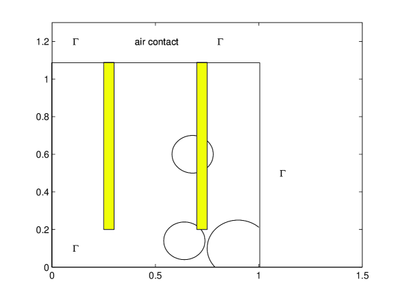
Figure 1. 2D schematic representations of a Lipschitz domain $\Omega$ (with $|\Omega|=1$) representing an electrolytic cell, $\Gamma$ being the union of the recipient and air contact boundaries, $\Gamma_{D}$ representing the surface of two electrodes submerged in the electrolyte, and $\Omega(x,r)=\Omega\cap B_{r}(x)$ denoting the subset centered at three different points

Finally, we state the following local version that will be required in Section 5. Here the boundary conditions do not play any role, since one can localize the problem around any point by multiplying with a suitable cut-off function, and paying for this by a modified variational formulation.

Proposition 4.5.

Let $n\geq 2$, $a\in L^{\infty}(\Omega)$ satisfies $0<a_{\#}\leq a\leq a^{\#}$ a.e. in $\Omega$, $x\in\Omega$, and $R>0$ be such that $|\Omega\cap\partial B_{R}(x)|>0$. If $u\in H^{1}(\Omega(x,R))$ solves the local variational formulation

(33) $$\int_{\Omega(x,R)}a\nabla u\cdot\nabla v\mathrm{dz}=0,\quad\forall v\in H^{1}_{\Omega\cap\partial B_{R}(x)}(\Omega(x,R)),$$

then we have

(34) $$\mathrel{\mathop{\kern 0.0pt{\rm ess}\sup}\limits_{\Omega(x,R/2)}}|u|\leq 2^{3n+2+{(3n)^{2}\over 4}}S_{2n\over n+2}^{3n/2}\left(R+1+2\sqrt{a^{\#}\over a_{\#}}\right)^{3n\over 2}{\omega_{n}\over R^{n/2}}\left(\int_{\Omega(x,R)}u^{2}\mathrm{dz}\right)^{1\over 2}.$$

Proof.

First we argue as in Proposition 4.3, with $k_{0}=0$. The validity of the properties (30) and (31) remain. The application of the $W^{1,2n/(n+2)}$-Sobolev inequality is available for $\eta(|u|-k)^{+}\in W^{1,2n/(n+2)}(A(x,R))$. Thus, we conclude the proof of Proposition 4.5 as in the proof of Proposition 4.4. ∎

5. Green kernels

In this Section, we reformulate some properties of the Green kernels.

Definition 5.1.

For each $x\in\Omega$, we say that $E$ is a Green kernel associated to (1)-(3), if it solves

(35) $$\nabla\cdot(a\nabla E(x,\cdot))=\delta_{x},$$

where $\delta_{x}$ is the Dirac delta function at the point $x$, in the following sense: there is $q>1$ such that $E$ verifies the variational formulation

(36) $$\int_{\Omega}a(y)\nabla_{y}E(x,y)\cdot\nabla_{y}v(y)\mathrm{dy}=v(x),\quad\forall v\in V_{q}.$$

If $|\Gamma_{D}|>0$, we call it the Green function, otherwise we call it simply the Neumann function (also called Green function for the Neumann problem or Green function of the second kind), and we write $E=G$ and $E=N$, respectively.

The existence of the Green function $G$ verifying

(37) $$G(x,y)=\lim_{\rho\rightarrow 0}G^{\rho}(x,y),\quad\forall x\in\Omega,\ \mbox{a.e. }y\in\Omega,\ x\not=y,$$

is standard if $n>2$ (see for instance [25, 31]), with $G^{\rho}(x,\cdot)\in H^{1}_{0}(\Omega)$ being the unique solution to

(38) $$\int_{\Omega}a\nabla G^{\rho}\cdot\nabla v\mathrm{dy}={1\over|B_{\rho}(x)|}\int_{B_{\rho}(x)}v\mathrm{dy},$$

for all $v\in H^{1}_{0}(\Omega)$, for any $x\in\Omega$, and $\rho>0$ such that $B_{\rho}(x)\subset\Omega$. Moreover, $G$ satisfies, for some positive constant $C(n)$, and $n>2$ [25, Theorem 1.1],

$$G(x,y)\leq C(n)(1+\log(a^{\#}/a_{\#})){(a^{\#})^{(n-2)/2}\over(a_{\#})^{n/2}|x-y|^{n-2}}.$$

In order to explicit the estimates and simultaneously to extend to $n=2$ and a mixed boundary value problem, let us build the Green kernels for $n\geq 2$.

Proposition 5.1.

Let $n\geq 2$, $1\leq q<n/(n-1)$, and $a$ be a measurable (and bounded) function defined in $\Omega$ satisfying $0<a_{\#}\leq a\leq a^{\#}$. Then, for each $x\in\Omega$ and any $r>0$ such that $r<{\rm dist}(x,\partial\Omega)$, there exists a unique Green function $G=G(x,\cdot)\in W^{1,q}_{\Gamma_{D}}(\Omega)\cap H^{1}(\Omega\setminus B_{r}(x))$ according to Definition 5.1, and enjoying the following estimates

(39) $$\|\nabla G\|_{q,\Omega}\leq C_{1}(\Omega,n,q)A+C_{2}(n,q,A);$$

(40) $$\|G\|_{qn/(n-q),\Omega}\leq S_{q}\left(C_{1}(\Omega,n,q)A+C_{2}(n,q,A)\right),$$

with $A=\sqrt{2/a_{\#}}$, and the constants $C_{1}(\Omega,n,q)$ and $C_{2}(n,q,A)$ being explicitly given in Proposition 3.3. Moreover, $G(x,y)\geq 0$ a.e. $x,y\in\Omega$, and

(41) $$|G(x,y)|\leq C(a_{\#})\left({\delta(\Omega)\over 2}+1+2\sqrt{a^{\#}\over a_{\#}}\right)^{3n/2}|x-y|^{1-n/q},$$

for a.e. $x,y\in\Omega$ such that $x\not=y$, where

$$C(a_{\#})=2^{3n+1+{n\over q}+{(3n)^{2}\over 4}}S_{2n\over n+2}^{3n/2}\omega_{n}^{{3\over 2}+{1\over n}-{1\over q}}S_{q}\left({C_{1}(\Omega,n,q)A}+C_{2}(n,q,A)\right).$$

Proof.

For any $x\in\Omega$, and $\rho>0$ such that $B_{\rho}(x)\subset\subset\Omega$, the existence and uniqueness of $G^{\rho}=G^{\rho}(x,\cdot)\in H^{1}_{\Gamma_{D}}(\Omega)$ solving (38), for all $v\in H^{1}_{\Gamma_{D}}(\Omega)$, are due to Proposition 3.1 with ${\bf f}={\bf 0}$ a.e. in $\Omega$, $g,h=0$ a.e. on, respectively, $\Gamma_{D}$ and $\Gamma$, and $f=\chi_{B_{\rho}(x)}/|B_{\rho}(x)|$ belonging to $L^{2n/(n+2)}(\Omega)$ if $n>2$, and to $L^{2}(\Omega)$ if $n=2$. Moreover, (3.1) reads

(42) $$\|\nabla G^{\rho}\|_{2,\Omega}\leq{1\over a_{\#}}\times\left\{\begin{array}[]{ll}S_{2}\omega_{n}^{1/n-1/2}\rho^{1-n/2}&\mbox{ if }n>2\\ |\Omega|^{1/2}(2\omega_{2}\rho^{2})^{-1/2}&\mbox{ if }n=2\end{array}\right..$$

Therefore, for any $r>0$ such that $B_{r}(x)\subset\subset\Omega$, there exists $G\in H^{1}(\Omega\setminus B_{r}(x))$ such that

$$G^{\rho}\rightharpoonup G\quad\mbox{in }H^{1}(\Omega\setminus B_{r}(x))\quad\mbox{ as $\rho\rightarrow 0^{+}$.}$$

In order to $G$ correspond to the well defined in (37), the $W^{1,q}$-estimate (39) is true for $G^{\rho}$ due to (3.3) with $\varkappa=2$, by applying Proposition 3.3 with ${\bf f}={\bf 0}$, $g,h=0$, and $f=\chi_{B_{\rho}(x)}/|B_{\rho}(x)|\in L^{1}(\Omega)$. Then, we can extract a subsequence of $G^{\rho},$ still denoted by $G^{\rho},$ weakly converging to $G$ in $W^{1,q}(\Omega)$ as $\rho$ tends to $0$, with $G\in V_{q}$ solving (36) for all $v\in V_{q^{\prime}}$. A well-known property of passage to the weak limit implies (39). The estimate (40) is consequence of the Sobolev embedding with continuity constant given in (6).

In order to prove the nonnegativeness assertion, first calculate

$$\int_{\Omega}a|\nabla(G^{\rho}-|G^{\rho}|)|^{2}\mathrm{dy}={2\over|B_{\rho}(x)|}\left(\int_{B_{\rho}(x)}G^{\rho}\mathrm{dy}-\int_{B_{\rho}(x)}|G^{\rho}|\mathrm{dy}\right)\leq 0.$$

Then, $G^{\rho}=|G^{\rho}|$, and by passing to the limit as $\rho$ tends to $0$, the nonnegativeness claim holds.

For each $x,y\in\Omega$ such that $x\not=y$, we may take $r<R=|x-y|/2$ such that $G(x,\cdot)\in H^{1}(\Omega(y,R))$ verifies $\nabla\cdot(a\nabla G)=0$ in $\Omega(y,R)$. Applying (34), followed by the Hölder inequality since $qn/(n-q)\geq 2$ means $q\geq 2n/(n+2)$, we obtain

$$|G(x,y)|\leq{C\over R^{n/2}}\left(\int_{\Omega(y,R)}G^{2}(x,z)\mathrm{dz}\right)^{1/2}$$

$$\leq C\omega_{n}^{{1/2}+{1/n}-{1/q}}R^{n\left({1/2}+{1/n}-{1/q}\right)-{n/2}}\|G\|_{qn/(n-q),\Omega},$$

with $C=2^{3n+2+{(3n)^{2}/4}}\left(\partial(\Omega)/2+1+2\sqrt{a^{\#}/a_{\#}}\right)^{3n/2}S_{2n/(n+2)}^{3n/2}\omega_{n}$.

Hence, using (40) we conclude (41), which completes the proof of Proposition 5.1. ∎

Remark 5.1.

Since $qn/(n-q)\rightarrow n/(n-1)$ as $q\rightarrow 1^{+}$, and $qn/(n-q)\rightarrow n/(n-2)$ as $q\rightarrow[n/(n-1)]^{-}$, the integrability exponent of $G$ in (40) obeys $n/(n-1)<qn/(n-q)<n/(n-2)$. In conclusion, Proposition 5.1 ensures that $G\in L^{p}(\Omega)$ for any $p\in[1,n/(n-2)[$.

For each $x\in\Omega$, the Neumann function is defined as $N=G+w$ being the solution of the regularity problem [27, Definition 2.5], where $G\in H^{1}_{0}(\Omega)$ is the Green function solving (38) and $w\in H^{1}(\Omega)$, with mean value zero over $\partial\Omega$, is the unique solution to the variational formulation [27, Lemma 2.3]

(43) $$\int_{\Omega}a\nabla w\cdot\nabla v\mathrm{dy}=-\int_{\partial\Omega}v\mathrm{ds_{y}}--\int_{\partial\Omega}v\mathrm{d}\omega_{\mathrm{y}}^{x},\quad\forall v\in V_{2}(\partial\Omega).$$

Here, $\omega^{x}$ is the L-harmonic measure [12], i.e. it is unique probability measure on $\partial\Omega$ such that

$$L_{g}(x)=\int_{\partial\Omega}g\mathrm{d}\omega_{\mathrm{y}}^{x},$$

due to the Riesz representation theorem applied to the continuous linear functional $L:g\in C(\partial\Omega)\rightarrow L_{g}(x)\in C(\bar{\Omega})$, where $L_{g}(x)$ is the solution to the Dirichlet problem (1) with ${\bf f}={\bf 0}$ and $f=0$, and (3) with $\Gamma_{D}=\partial\Omega$. The question of solvability of the regularity problem is assigned by the gradient of the solution having nontangential limits at almost every point of the boundary [18, 27].

Remark 5.2.

For each $x\in\Omega$, $N(x,\cdot)$ admits an extension $\widetilde{N}(x,\cdot)$ across $\partial\Omega$ (cf. [27, Lemmas 2.9 and 2.11]) to the domain $\widetilde{\Omega}$ which is such that

$$y\in\partial\widetilde{\Omega}\Leftrightarrow y\in\mathbb{R}^{n}\setminus\bar{\Omega}:\quad y=y^{*}+(y^{*}-{\mathcal{T}}(y^{*})),\quad\mbox{ for some }y^{*}\in\partial\Omega,$$

where $\mathcal{T}$ is the homothety function that reduces $\partial\Omega$ into its half, i.e. the homothetic boundary with measure $|\partial\Omega|/2$. That is, each $y\in\widetilde{\Omega}\setminus\bar{\Omega}$ is the reflection of $\mathcal{T}(y^{\delta})$ across $\partial\Omega$ in the following sense:

$$y=y^{*}+(y^{*}-y^{\delta}){y^{*}-\mathcal{T}(y^{*})\over|y^{*}-\mathcal{T}(y^{*})|},$$

where $y^{\delta}\in\Omega$ is such that $y^{\delta}=y^{*}-\delta(y^{*}-\mathcal{T}(y^{*}))/|y^{*}-\mathcal{T}(y^{*})|$, for some $0<\delta<\delta(\Omega)$.

Since our concern is on weak solutions to (1)-(3) in accordance with Definition 2.1, we reformulate for $n\geq 2$ the existence result due to Kenig and Pipher on solutions to the Neumann problem in bounded Lipschitz domains if $n>2$, with no information of its boundary behavior.

Proposition 5.2.

Let $n\geq 2$, $1\leq q<n/(n-1)$, and $a$ be a measurable (and bounded) function defined in $\Omega$ satisfying $0<a_{\#}\leq a\leq a^{\#}$. Then, for each $x\in\Omega$, there exists a Neumann function $N=N(x,\cdot)\in V_{q}$ solving (35) that satisfies (39)-(40), and (41), with $A=2/\sqrt{a_{\#}}$.

Proof.

For each $x\in\Omega$, and $\rho>0$ such that $B_{\rho}(x)\subset\Omega$, the existence of a unique Neumann function $N^{\rho}(x,\cdot)\in V_{2}$ solving (38), for all $v\in V_{2}$, is consequence of Proposition 3.2 with ${\bf f}={\bf 0}$, $g,h=0$, and $f=\chi_{B_{\rho}(x)}/|B_{\rho}(x)|\in L^{t}(\Omega)$ for $t=2n/(n+2)$ if $n>2$, and any $t<2$ if $n=2$. Arguing as in the proof of Proposition 5.1, $N^{\rho}$ belongs to $W^{1,q}(\Omega)$, uniformly for $x\in\Omega$, according to (3.3) with $\varkappa=4$. Therefore, we may pass to the limit as $\rho\rightarrow 0$, finding $N\in V_{q}$ solving (35). The remaining estimates (40)-(41), under $A=2/\sqrt{a_{\#}}$, are obtained exactly as in the proof of Proposition 4.4. ∎

Hereafter, $\partial_{x_{i}}$ denotes the partial derivative $\partial/\partial x_{i}$.

Proposition 5.3.

Let $n\geq 2$, $1\leq q<n/(n-1)$, $E$ be the symmetric function that is either the Green function $G$ or the Neumann function $N$ in accordance with Propositions 5.1 and 5.2, respectively. If $a\in L^{\infty}(\Omega)$ verifies $0<a_{\#}\leq a\leq a^{\#}$ a.e. in $\Omega$, then for every $i=1,\cdots,n$ $\partial_{x_{i}}E(x,\cdot)\in V_{q}\cap L^{\infty}(\Omega)$ is uniformly bounded for $x\in\Omega$. In particular, it satisfies (39)-(40), and (41), where $A=\sqrt{\varkappa/a_{\#}}$, with $\varkappa=2$ if $|\Gamma_{D}|>0$, and $\varkappa=4$ if $|\Gamma_{D}|=0$.

Proof.

For each $x\in\Omega$, we may approximate $\partial_{x_{i}}E(x,\cdot)$ by $\{\partial_{x_{i}}E^{\rho}\}_{\rho>0}$, where $E^{\rho}=E^{\rho}(x,\cdot)\in V_{2}$ solves (38) for every $\rho>0$ such that $B_{\rho}(x)\subset\Omega$. Since $\partial_{x_{i}}[\chi_{B_{\rho}(x)}/(\rho^{n}|B_{1}(0)|)]$ is a Dirac delta function, Proposition 3.4 ensures that $\partial_{x_{i}}E^{\rho}$ verifies (39), and also (40) by the Sobolev inequality (6), with $A=\sqrt{\varkappa/a_{\#}}$, where $\varkappa=2$ if $|\Gamma_{D}|>0$, and $\varkappa=4$ if $|\Gamma_{D}|=0$. Consequently, (39)-(40) hold, by passage to the weak limit.

To prove the estimate (41) for $\partial_{x_{i}}E(x,\cdot)$, let us take $y\in\Omega$ such that $R=|x-y|/2>0$. Thus, $E(x,\cdot)\in H^{1}(\Omega(y,R))\cap V_{q}$ verifies $\nabla\cdot(a\nabla\partial_{x_{i}}E)=0$ in $\Omega(y,R)$, for every $i=1,\cdots,n$. Therefore, we proceed by using the argument already used in the proof of Proposition 5.1, with $G$ replaced by $\partial_{x_{i}}E$. ∎

Remark 5.3.

Notice that $q^{\prime}>n$ implies that $E$ is not an admissible test function in

$$\int_{\Omega}a(y)\nabla\partial_{x_{i}}E(x,y)\cdot\nabla v(y)\mathrm{dy}=\partial_{x_{i}}v(x),\quad\forall v\in V_{q^{\prime}},$$

for each $x\in\Omega$, and for every $i=1,\cdots,n$, which comes from Definition 5.1, i.e. due to differentiate (36) under the integral sign in $x_{i}$. We emphasize that for each $x\in\Omega$ and any $r>0$ such that $r<{\rm dist}(x,\partial\Omega)$, the symmetric function $E(x,\cdot)\in V_{q}\cap H^{1}(\Omega\setminus B_{r}(x))$ verifies, by construction, the limit system of identities

$$\int_{\Omega}a\varphi^{2}\nabla(\nabla_{x}E)(x,\cdot)\cdot\nabla v\mathrm{dz}=-2\int_{\Omega}a\varphi v\nabla(\nabla_{x}E)(x,\cdot)\cdot\nabla\varphi\mathrm{dz},$$

for any $\varphi\in W^{1,\infty}(\mathbb{R}^{n})$ such that supp$(\varphi)\subset\mathbb{R}^{n}\setminus\overline{B_{\partial(\Omega)}(x)\cup B_{r}(x)}$, and for all $v\in V_{1}\cap H^{1}(\Omega\cap\mathrm{supp}(\varphi))$.

Next, we prove additional estimates for the derivative of the weak solution to (1) with ${\bf f}={\bf 0}$ and $f=0$, if we strengthen the hypotheses on the regularity of the coefficient $a$. Indeed we proceed as in [25] where the coefficient is assumed Dini-continuous to be enable to derive some more pointwise estimates for the derivative of the Green kernels.

Proposition 5.4.

Let $a\in L^{\infty}(\Omega)$ satisfy $0<a_{\#}\leq a\leq a^{\#}$ a.e. in $\Omega$. If there exists a function $\omega:[0,\infty[\rightarrow[0,\infty[$ such that, a.e. $x,y\in\Omega$,

(44) $$|a(x)-a(y)|\leq\omega(|x-y|),\quad 0<C_{a}:=\int_{0}^{1}{\omega(t)\over t}\mathrm{dt}<\infty$$

then for each $x\in\Omega$, and $R>0$, any function $u\in W^{1,1}(\Omega)$ solving

(45) $$\nabla\cdot(a\nabla u)=0\mbox{ in }\Omega(x,R),$$

in the sense of distributions, enjoys a.e. $y\in\Omega$,

(46) $$|\nabla u(y)|\leq{a_{\#}\delta(\Omega)\over C_{a}n\omega_{n}}\left({4\pi\over 3}+n\right){1\over|x-y|}\int_{B_{d}(y)}{|u(z)|\over|y-z|^{n}}\mathrm{dz},$$

where

(47) $$d=\left\{\begin{array}[]{ll}|x-y|/2,&\mbox{if }|x-y|<2r\\ |x-y|/\nu,&\mbox{if }|x-y|=\nu r\end{array}\right.$$

for some $2\leq\nu<\delta(\Omega)/r$ and $0<r<\min\{1,\delta(y)\}$ with $\delta(y):={\rm dist}(y,\partial\Omega)$.

Proof.

By density, since $u\in W^{1,1}(\Omega)$ there exists a sequence $\{u_{m}\}_{m\in\mathbb{N}}\subset C^{1}(\bar{\Omega})$ such that $u_{m}\rightarrow u$ in $W^{1,1}(\Omega)$. In particular, $u_{m}\rightarrow u$ in $L^{1}(\Omega)$ and $\nabla u_{m}\rightarrow\nabla u$ a.e. in $\Omega$. Thus, it is sufficient to prove the estimate (46), under the assumption $u\in C^{1}(\bar{\Omega})$.

Fix $x\in\Omega$, and $R>0$. For an arbitrary $y\in\Omega(x,R)$ we can choose $0<r<\min\{R,1,\delta(y)\}$ and $M>0$ such that

(48) $$\sup_{z\in B_{r}(y)}|x-z||\nabla u(z)|=M\quad\mbox{ and }\quad|x-y||\nabla u(y)|>2bM,$$

for some constant $b\in]0,1/2[$. Since $\Omega$ is bounded, we can take $2\leq\nu<\delta(\Omega)/r$ and define $d$ as in (47). Notice that $d\leq r$ implies $B_{d}(y)\subset\subset\Omega$.

In order to determine the final constant in (46), let $\eta\in C^{1}_{0}(B_{d}(y))\cap W^{2,\infty}(\Omega)$ be the cut-off function explicitly given by

$$\eta(z)=\left\{\begin{array}[]{ll}1,&\mbox{ if }z\in B_{d/2}(y)\\ 2^{-1}\left(1+\cos\Big{[}{4\pi\over 3d^{2}}(|z-y|^{2}-d^{2}/4)\Big{]}\right),&\mbox{ if }d/2\leq|z-y|<d\\ 0,&\mbox{ if }z\in\Omega\setminus B_{d}(y).\end{array}\right.$$

Thus, $\eta$ satisfies $0\leq\eta\leq 1$,

(49) $$|\nabla\eta(z)|\leq{c_{1}/d}\leq c_{1}\nu|x-y|^{-1}, \forall z\in\Omega (c_{1}={4\pi/3})$$

(50) $$\qquad|\Delta\eta(z)|\leq{c_{1}c_{2}/d^{2}}\leq c_{1}c_{2}\nu^{2}|x-y|^{-2}, \mbox{a.e. }z\in\Omega (c_{2}=c_{1}+n).$$

For $w\in B:=B_{d}(y)$, we multiply (45) by $G_{L}(w,\cdot)\eta/a(y)$ where $G_{L}$ is the fundamental solution of Laplace equation,

$$G_{L}(w,z)=C_{L}\left\{\begin{array}[]{ll}(2-n)^{-1}|w-z|^{2-n}&\mbox{if }n>2\\ \ln[|w-z|]&\mbox{if }n=2\end{array}\right.$$

with

(51) $$C_{L}:={ba_{\#}r\over(c_{1}\nu+2(n+1))C_{a}n\omega_{n}},$$

and we integrate over $B$ to get

$$0=\int_{B}{a(z)\over a(y)}\nabla_{z}u(z)\cdot\nabla_{z}(\eta(z)G_{L}(w,z))\mathrm{dz}$$

$$=\int_{B}{a(z)-a(y)\over a(y)}\nabla_{z}u(z)\cdot\nabla_{z}(\eta(z)G_{L}(w,z))\mathrm{dz}-\int_{B}u\Delta_{z}\eta G_{L}(w,\cdot)\mathrm{dz}$$

$$-2\int_{B}u(z)\nabla_{z}\eta(z)\cdot\nabla_{z}G_{L}(w,z)\mathrm{dz}-u(w)\eta(w),$$

taking into account the use of integration by parts. Differentiating the above identity with respect to $w$ and setting $w=y$ it results in

$$\nabla u(y)=I_{1}+I_{2},$$

where

$$I_{1}= \int_{B}{a(z)-a(y)\over a(y)}\Big{(}\nabla_{y}G_{L}(y,z)\nabla_{z}\eta(z)+\eta(z)\nabla_{y}\nabla_{z}G_{L}(y,z)\Big{)}\cdot\nabla_{z}u(z)\mathrm{dz};$$

$$I_{2}= -\int_{B}u(z)\nabla_{y}G_{L}(y,z)\Delta_{z}\eta(z)\mathrm{dz}-2\int_{B}u(z)\nabla_{y}\nabla_{z}G_{L}(y,z)\cdot\nabla_{z}\eta(z)\mathrm{dz}.$$

Using the lower bound of $a$, the definition of $G_{L}$, and the properties of $\eta$, we have

$$I_{1}\leq{C_{L}\over a_{\#}}\int_{B}|a(z)-a(y)|\left({c_{1}\nu\over|y-z|^{n-1}|x-y|}+{n+1\over|y-z|^{n}}\right)|\nabla_{z}u(z)|\mathrm{dz};$$

$$I_{2}\leq C_{L}c_{1}\nu\int_{B}|u(z)|\left({c_{2}\nu\over|y-z|^{n-1}|x-y|^{2}}+{2(n+1)\over|y-z|^{n}|x-y|}\right)\mathrm{dz}.$$

By appealing to (48), we obtain

$$2bM<|x-y||\nabla u(y)|\leq$$

$$\leq{C_{L}M\over a_{\#}}\int_{B}{|a(z)-a(y)|\over|x-z|}\left({c_{1}\nu\over|y-z|^{n-1}}+(n+1){|x-y|\over|y-z|^{n}}\right)\mathrm{dz}+$$

$$+C_{L}c_{1}\nu\int_{B}|u(z)|\left({c_{2}\nu\over|y-z|^{n-1}|x-y|}+{2(n+1)\over|y-z|^{n}}\right)\mathrm{dz}.$$

Considering that, for all $x,y\in\Omega$ and $z\in B_{d}(y)$,

$$|y-z|\leq|x-y|\leq|x-z|+|z-y|$$

we obtain

(52) $$2bM<{C_{L}M\over a_{\#}}\left(\int_{B}{|a(z)-a(y)|}{c_{1}\nu+n+1\over|y-z|^{n-1}|x-z|}\mathrm{dz}+\right.$$

$$\left.+(n+1)\int_{B}{|a(z)-a(y)|\over|y-z|^{n}}\mathrm{dz}\right)+C_{L}c_{1}\nu\left(c_{2}\nu+2(n+1)\right)\int_{B}{|u(z)|\over|y-z|^{n}}\mathrm{dz}.$$

Let us analyze the first integral of RHS in (52). From the definition of the radius $d$, we consider two different cases: $|x-y|=\nu r$ and otherwise. In the first case, from $z\in B_{d}(y)$ we have $|y-z|<|x-y|/\nu$. Hence, we find $(\nu-1)|y-z|<|x-z|$ and consequently

(53) $${1\over|y-z|^{n-1}|x-z|}<{1\over(\nu-1)|y-z|^{n}}\leq{1\over|y-z|^{n}},\qquad\nu\geq 2.$$

If $d=|x-y|/2$ and $z\in B_{d}(y)$, clearly (53) holds denoting $\nu=2$.

Returning to (52), substituting the value of $C_{L}$ from (51) with $r\leq 1$, and dividing by $b>0$, we write it as

(54) $$2M<{M\over C_{a}n\omega_{n}}\int_{B}{|a(z)-a(y)|\over|y-z|^{n}}\mathrm{dz}+{a_{\#}\delta(\Omega)c_{1}\over C_{a}n\omega_{n}}\left(1+{n\over c_{1}}\right)\int_{B}{|u(z)|\over|y-z|^{n}}\mathrm{dz}.$$

In a $n$-dimensional Euclidean space, the spherical coordinate system consists of a radial coordinate $t$, and $n-1$ angular coordinates $\phi_{1},\cdots,\phi_{n-2}\in[0,\pi]$, and $\phi_{n-1}\in[0,2\pi[$, and the Cartesian coordinates are $z_{1}=y_{1}+t\cos(\phi_{1})$, $z_{2}=y_{2}+t\sin(\phi_{1})\cos(\phi_{2})$, $\cdots,$ $z_{n-1}=y_{n-1}+t\sin(\phi_{1})\cdots\sin(\phi_{n-2})\cos(\phi_{n-1})$, and $z_{n}=y_{n}+t\sin(\phi_{1})\cdots\sin(\phi_{n-1})$. Since the Jacobian of this transformation is $t^{n-1}\sin^{n-2}(\phi_{1})\sin^{n-3}(\phi_{2})\cdots\sin(\phi_{n-2})$, and

$$\omega_{n}={1\over n}\int_{0}^{\pi}\cdots\int_{0}^{\pi}\int_{0}^{2\pi}\sin^{n-2}(\phi_{1})\sin^{n-3}(\phi_{2})\cdots\sin(\phi_{n-2})\mathrm{d\phi_{1}}\cdots\mathrm{d\phi_{n-1}},$$

applying (44), we deduce

(55) $$\int_{B}{|a(z)-a(y)|\over|y-z|^{n}}\mathrm{dz}\leq\int_{B}{\omega(|y-z|)\over|y-z|^{n}}\mathrm{dz}=n\omega_{n}\int_{0}^{d}{\omega(t)\over t}\mathrm{dt}\leq C_{a}n\omega_{n}.$$

Inserting this last inequality into (54), we find (46). ∎

Remark 5.4.

Observing (55), the assumption (44) can be replaced by $a$ belonging to the VMO space of vanishing mean oscillation functions which is constituted by the functions $f$ belonging to the BMO space such that verify

$$\lim_{r\rightarrow 0}\sup_{\rho\leq r}-\int_{B_{\rho}}|f(x)-\Big{(}-\int_{B_{\rho}}f(y)\mathrm{dy}\Big{)}|\mathrm{dx}=0,$$

where $B_{\rho}$ ranges in the class of the balls with radius $\rho$ contained in $\Omega$. We recall that the John-Nirenberg space BMO of the functions of bounded mean oscillation is defined as

$$BMO=\{f\in L^{1}_{\rm loc}(\Omega):\ \sup_{B}-\int_{B}|f(x)-\Big{(}-\int_{B}f(y)\mathrm{dy}\Big{)}\mathrm{dx}<\infty\},$$

where $B$ ranges in the class of the balls contained in $\Omega$.

Remark 5.5.

The upper bound in (46) is not optimal, it depends on the choice of the cut-off function through the contants $c_{1}$ and $c_{2}$ (cf. (49)-(50) and (54)).

Proposition 5.5.

Let $n\geq 2$, $1\leq q<n/(n-1)$, $E$ be the symmetric function that is either the Green function $G$ or the Neumann function $N$ in accordance with Propositions 5.1 and 5.2, respectively. If $a\in L^{\infty}(\Omega)$ satisfies $0<a_{\#}\leq a\leq a^{\#}$ a.e. in $\Omega$, and (44), then a.e. $x,y\in\Omega$,

(56) $$|\nabla_{y}E(x,y)|\leq C(\Omega,n,q,a)|x-y|^{-n/q},$$

with

$$C(\Omega,n,q,a)={\delta(\Omega)\over C_{a}}(4{\pi\over 3}+n)2^{3n+2{n/q}+{(3n)^{2}/4}}S_{2n\over n+2}^{3n/2}\omega_{n}^{{1/n}-{1/q}+{3/2}}S_{q}\times$$

$$\times\left(C_{1}(\Omega,n,q)\sqrt{\varkappa a_{\#}}+a_{\#}C_{2}(n,q,\sqrt{\varkappa\over a_{\#}})\right)\left({\delta(\Omega)\over 2}+1+2\sqrt{a^{\#}\over a_{\#}}\right)^{3n\over 2},$$

where $\varkappa=2$ if $|\Gamma_{D}|>0$, $\varkappa=4$ if $|\Gamma_{D}|=0$, and the constants $C_{1}(\Omega,n,q)$ and $C_{2}(n,q,\sqrt{\varkappa/a_{\#}})$ are explicitly given in Proposition 3.3.

Proof.

Let $x\in\Omega$ be arbitrary. Using the property (46), and applying (41), we get

$$|\nabla_{y}E(x,y)|\leq{\delta(\Omega)\over C_{a}}\left(C_{1}(\Omega,n,q)\sqrt{\varkappa a_{\#}}+a_{\#}C_{2}(n,q,\sqrt{\varkappa\over a_{\#}})\right){C\over|x-y|}\times$$

$$\times\left({\partial(\Omega)\over 2}+1+2\sqrt{a^{\#}\over a_{\#}}\right)^{3n/2}\int_{B_{d}(y)}{|x-z|^{1-n/q}\over|y-z|^{n}}\mathrm{dz},$$

with

$$C=(4{\pi\over 3}+n)2^{3n+1+{n/q}+{(3n)^{2}/4}}S_{2n/(n+2)}^{3n/2}{\omega_{n}^{{1/n}-{1/q}+{1/2}}\over n}S_{q}.$$

Considering that, for all $x,y\in\Omega$ and $z\in B_{d}(y)$ with $d\leq|x-y|/2$,

$$|y-z|\leq{|x-y|\over 2}\leq{1\over 2}(|x-z|+|z-y|)\Longrightarrow\left\{\begin{array}[]{l}|y-z|\leq|x-z|\\ |x-y|\leq 2|x-z|\end{array}\right.,$$

we compute

$$\int_{B_{d}(y)}{|x-z|^{1-{n\over q}}\over|y-z|^{n}}\mathrm{dz}\leq 2^{n/q}\int_{B_{d}(y)}{|x-y|^{-n/q}\over|y-z|^{n-1}}\mathrm{dz}=2^{n/q}dn\omega_{n}|x-y|^{-n/q},$$

where the Riesz potential is calculated by the spherical transformation as in the above proof. Next, from $d\leq|x-y|/2$ we find (56).∎

6. $W^{1,p}$-constants ($p>n$)

Let $p>n$, $g=0$ on $\Gamma_{D}$ (possibly empty), and $u\in V_{p}$ solve (9) for all $v\in V_{p^{\prime}}$. Its existence depends on several factors.

The regularity theory for solutions of the class of divergence form elliptic equations in convex domains guarantees the existence of a unique strong solution if the coefficient is uniformly continuous, taking the Korn perturbation method [22, pp. 107-109] into account. This result can be proved if the convexity of $\Omega$ is replaced by weaker assumptions, for instance when $\Omega$ is a plane bounded domain with Lipschitz and piecewise $C^{2}$ boundary whose angles are all convex [22, p. 151], or when $\Omega$ is a plane bounded domain with curvilinear polygonal $C^{1,1}$ boundary whose angles are all strictly convex [22, p. 174]. For general bounded domains with Lipschitz boundary, the higher integrability of the exponents for the gradients of the solutions may be assured [2, 39], under particular restrictions on the coefficients. In [17, 26], the authors figure out configurations of (discontinuous) coefficient functions and geometries of the domain, such that the required result does hold. In [29], the authors derive global $W^{1,\infty}$ and piecewise $C^{1,\alpha}$ estimates with piecewise Hölder continuous coefficients, which depend on the shape and on the size of the surfaces of discontinuity of the coefficients, but they are independent of the distance between these surfaces. When the coefficient of the principal part of the divergence form elliptic equation is only supposed to be bounded and measurable, Meyers extends Boyarskii result to n-dimensional elliptic equations of divergence structure [32]. Adopting this rather weak hypothesis, the works [23, 24, 34] extend to mixed boundary value problem the result due to Meyers.

For a domain of class $C^{1,1}$, $W^{1,p}$-regularity of the solution is found for $1<p<\infty$ in [15, 36] under the hypotheses on the coefficients of the principal part are to belong to the Sarason class [37] of vanishing mean oscillation functions (VMO). In [19], the author extends the $W^{1,p}$-solvability to the Neumann problem for a range of integrability exponent $p\in]2n/(n+1)-\varepsilon,2n/(n-1)+\varepsilon[$, where $\varepsilon>0$ depends on $n$, the ellipticity constant, and the Lipschitz character of $\Omega$. Notwithstanding, the results concerning VMO-coefficients are irrevelant for real world applications. The reason is that the VMO-property forbids jumps across a hypersurface, what is the generic case of discontinuity.

For Lipschitz domains with small Lipschitz constant, the Neumann problem is solved in [16], where the leading coefficient is assumed to be measurable in one direction, to have small BMO semi-norm in the other directions, and to have small BMO semi-norm in a neighborhood of the boundary of the domain. We refer to [6] for the optimal $W^{1,p}$ regularity theory regarding Dirichlet problem on bounded domains whose boundary is so rough that the unit normal vector is not well defined, but is well approximated by hyperplanes at every point and at every scale (Reifenberg flat domain); and the coefficient belongs to the space $\mathcal{V}$ such that $C(\Omega)\subset$ VMO $\subset\mathcal{V}\subset$ BMO which is defined as the BMO space with their BMO semi-norms sufficiently small. In [7] the authors obtain the global $W^{1,p}$ regularity theory a linear elliptic equation in divergence form with the conormal boundary condition via perturbation theory in harmonic analysis and geometric measure theory, in particular on maximal function approach.

Let us begin by establishing the relation between any weak solution $u\in V_{p}$ ($p>n$) and the Green kernel $E$ associated to (1)-(3), i.e. $E\in V_{p^{\prime}}$ is either the Green or the Neumann functions, $E=G$ and $E=N$, in accordance with Propositions 5.1 and 5.2, respectively. To this end, we take $v=E\in V_{p^{\prime}}$ and $v=u\in V_{p}$ as test functions in (9) and (36), respectively, obtaining the Green representation formula

(57) $$u(x)=\mathcal{T}({\bf f})(x)+\mathcal{S}(f)(x)+\mathcal{K}(h)(x),\qquad x\in\Omega,$$

where $\mathcal{T}$, $\mathcal{S}$, and $\mathcal{K}$ are the layer potential operators defined by

$$\mathcal{T}({\bf f}) = \sum_{j=1}^{n}\int_{\Omega}f_{j}(y){\partial E\over\partial{y_{j}}}(\cdot,y)\mathrm{dy};$$

$$\mathcal{S}(f) = \int_{\Omega}f(y)E(\cdot,y)\mathrm{dy};$$

$$\mathcal{K}(h) = \int_{\partial\Omega}\chi_{\Gamma}(y)h(y)E(\cdot,y)\mathrm{ds_{y}}.$$

For every $0<\lambda<n$, $u\in L^{s}(\mathbb{R}^{n})$, $v\in L^{t}(\mathbb{R}^{n})$, with $s,t>1$ and $\lambda/n+1/s+1/t=2$, the Hardy-Littlewood-Sobolev inequality in its general form states the following:

(58) $$\int_{\mathbb{R}^{n}}\int_{\mathbb{R}^{n}}u(x)|x-y|^{-\lambda}v(y)\mathrm{dx}\mathrm{dy}\leq C(n,s,\lambda)\|u\|_{s,\mathbb{R}^{n}}\|v\|_{t,\mathbb{R}^{n}},$$

where the constant is sharp [30], if $s=t=2n/(2n-\lambda)$, defined by

$$C(n,\lambda)=\pi^{\lambda/2}{\Gamma((n-\lambda)/2)\over\Gamma(n-\lambda/2)}\left[{\Gamma(n)\over\Gamma(n/2)}\right]^{1-\lambda/n}.$$

In the presence of the Hardy-Littlewood-Sobolev inequality, we prove the following $W^{1,p}$-estimate.

Proposition 6.1.

Let $p>1$, $f\in L^{t}(\Omega)$ with $t\in]pn/(p+n),p[$, ${\bf f}={\bf 0}$ in $\Omega$, $g=0$ on $\Gamma_{D}$ (possibly empty), $h=0$ on $\Gamma$, $a\in L^{\infty}(\Omega)$ satisfy $0<a_{\#}\leq a\leq a^{\#}$ a.e. in $\Omega$, and (44). If $u\in V_{p}$ solves (9), for all $v\in V_{p^{\prime}}$, then $u$ satisfies

(59) $$\|\nabla u\|_{p,\Omega}\leq C(n,p^{\prime},n/q)C(\Omega,n,q,a)\|f\|_{t,\Omega},$$

with $1/q=1+1/p-1/t$, $C(n,p^{\prime},n/q)$ relative to (58), and $C(\Omega,n,q,a)$ determined in Proposition 5.5. In particular, for $2<p<2n/(n-1)$ we have

$$\|\nabla u\|_{p,\Omega}\leq C(n,2n/p)C(\Omega,n,p/2,a)\|f\|_{p^{\prime},\Omega}.$$

Proof.

Since $\nabla u\in{\bf L}^{p}(\Omega)$, (57) holds. Differentiating it, for $i=1,\cdots,n$, we deduce

$${\partial u\over\partial x_{i}}(x)=\int_{\Omega}{\partial E\over\partial x_{i}}(x,y){f(y)}\mathrm{dy}.$$

Let ${\bf w}\in{\bf L}^{p^{\prime}}(\Omega)$ be arbitrary such that $\|{\bf w}\|_{p^{\prime},\Omega}=1$. Using (56) for any $1<q<n/(n-1)$, and applying the Fubini-Tonelli Theorem, we find

$$\int_{\Omega}\nabla u(x)\cdot{\bf w}(x)\mathrm{dx}\leq C(\Omega,n,q,a)\int_{\Omega}\int_{\Omega}|{\bf w}(x)||x-y|^{-n/q}|f(y)|\mathrm{dx}\mathrm{dy}.$$

Next, using (58) with $\lambda=n/q$, $s=p^{\prime}$, and $1/t=1+1/p-1/q$, we conclude (59).

For the particular situation, we choose $1<q=p/2<n/(n-1)$ and we use (58) with $s=t=p^{\prime}$. ∎

Having the results established in Section 5 in mind, we find a $W^{1,p}$-estimate for weak solutions where the regularity (44) of the leading coefficient is not a necessary condition.

Proposition 6.2.

Let $p>n$, ${\bf f}\in{\bf L}^{p}(\Omega)$, $f\in L^{p}(\Omega)$, $g=0$ on $\Gamma_{D}$ (possibly empty), $h\in L^{p}(\Gamma)$, $a\in L^{\infty}(\Omega)$ satisfy $0<a_{\#}\leq a\leq a^{\#}$ a.e. in $\Omega$, and $u\in V_{p}$ solve (9), for all $v\in V_{p^{\prime}}$. Then $u$ satisfies

$$\|\nabla u\|_{p,\Omega}\leq|\Omega|^{1/p}\left({C_{1}(\Omega,n,p^{\prime})\over a_{\#}}+C_{2}(n,p^{\prime},{1\over a_{\#}})\right)\times$$

$$\times(\|{\bf f}\|_{p,\Omega}+\|f\|_{p,\Omega}+|\Gamma|^{1/[p/n-1)]}K_{p^{\prime}}\|h\|_{p,\partial\Omega}),$$

with the constants $C_{1}(\Omega,n,p^{\prime})$ and $C_{2}(n,p^{\prime},1/a_{\#})$ being explicitly given in Proposition 3.3.

Proof.

Differentiating (57), for $i=1,\cdots,n$, we deduce

$${\partial u\over\partial x_{i}}(x)=\sum_{j=1}^{n}\int_{\Omega}{\partial^{2}E\over\partial x_{i}\partial y_{j}}(x,\cdot){f_{j}}\mathrm{dy}+\int_{\Omega}{\partial E\over\partial x_{i}}(x,\cdot){f}\mathrm{dy}+\int_{\Gamma}{\partial E\over\partial x_{i}}(x,\cdot){h}\mathrm{ds_{y}}.$$

Let ${\bf w}\in{\bf L}^{p^{\prime}}(\Omega)$ be arbitrary such that $\|{\bf w}\|_{p^{\prime},\Omega}=1$, applying the Fubini-Tonelli Theorem and next the Hölder inequality, it follows

(60) $$\qquad\int_{\Omega}\nabla u\cdot{\bf w}\mathrm{dx}\leq\|{\bf f}\|_{p,\Omega}\left(\int_{\Omega}\left|\sum_{i,j=1}^{n}\int_{\Omega}{\partial^{2}E\over\partial x_{i}\partial y_{j}}(\cdot,y)w_{i}\mathrm{dx}\right|^{p^{\prime}}\mathrm{dy}\right)^{1/p^{\prime}}$$

$$+\|f\|_{p,\Omega}\left(\int_{\Omega}\left|\sum_{i=1}^{n}\int_{\Omega}{\partial E\over\partial x_{i}}(\cdot,y)w_{i}\mathrm{dx}\right|^{p^{\prime}}\mathrm{dy}\right)^{1/p^{\prime}}$$

$$+\|h\|_{p,\Gamma}\left(\int_{\Gamma}\left|\sum_{i=1}^{n}\int_{\Omega}{\partial E\over\partial x_{i}}(\cdot,y)w_{i}\mathrm{dx}\right|^{p^{\prime}}\mathrm{ds_{y}}\right)^{1/p^{\prime}}.$$

Let us estimate the last integral on RHS in (60), since the two others integrals are similarly bounded,

$$\mathcal{I}:=\left(\int_{\Gamma}\left|\int_{\Omega}\sum_{i=1}^{n}{\partial E\over\partial x_{i}}(x,y)w_{i}(x)\mathrm{dx}\right|^{p^{\prime}}\mathrm{ds_{y}}\right)^{1/p^{\prime}}\leq$$

$$\leq|\Omega|^{1/p}\left(\int_{\Omega}\left(\int_{\Gamma}|\nabla_{x}E(x,y)|^{p^{\prime}}\mathrm{ds_{y}}\right)|{\bf w}(x)|^{p^{\prime}}\mathrm{dx}\right)^{1/p^{\prime}},$$

where $|\Omega|^{1/p}$ is due to the embedding $L^{p^{\prime}}(\Omega)\hookrightarrow L^{1}(\Omega)$. Considering that $\partial_{x_{i}}E(x,\cdot)\in W^{1,p^{\prime}}(\Omega)$ uniformly for $x\in\Omega$ (cf. Proposition 5.3), consequently also $\nabla_{x}E(x,\cdot)\in{\bf W}^{1,p^{\prime}}(\Omega)\hookrightarrow{\bf L}^{p^{\prime}(n-1)/(n-p^{\prime})}(\Gamma)\hookrightarrow{\bf L}^{p^{\prime}}(\Gamma)$ uniformly in $x\in\Omega$, then we obtain

$$\mathcal{I}\leq|\Omega|^{1/p}|\Gamma|^{1/[p(n-1)]}K_{p^{\prime}}\left({C_{1}(\Omega,n,p^{\prime})\over a_{\#}}+C_{2}(n,p^{\prime},1/a_{\#})\right).$$

Finally, inserting the above inequality into (60), the proof of Proposition 6.2 is finished. ∎

References

- [1] S. Agmon, A. Douglis and L. Nirenberg, Estimates near the boundary for solutions of elliptic partial differential equations satisfying general boundary conditions I, Comm. Pure Appl. Math. 12 (1959), 623-727.
- [2] M.S. Agranovich, Regularity of variational solutions to linear boundary value problems in Lipschitz domains, Functional Analysis and Its Applications 40 :4 (2006), 313-329, Translated from Funktsional’nyi Analiz i Ego Prilozheniya, Vol. 40, No. 4 (2006), 83-103.
- [3] H. Beirão da Veiga, Sur la regularité des solutions de l’équation avec des conditions aux limites unilaterales et melées, Ann. Mat. Pura Appl. 93 (1972), 173-230.
- [4] L. Boccardo and T. Gallouët, Non-linear elliptic and parabolic equations involving measure, Journal of Functional Analysis 87 (1989), 149-169.
- [5] J.F. Bonder and N. Saintier, Estimates for the Sobolev trace constant with critical exponent and applications, Ann. Mat. Pura Appl. 187 :4 (2008), 683-704.
- [6] S.-S. Byun and L. Wang, Elliptic equations with BMO coefficients in Reifenberg domains, Comm. Pure Appl. Math. 57 :10 (2004), 1283-1310.
- [7] S.-S. Byun and L. Wang, The conormal derivative problem for elliptic equations with BMO coefficients on Reifenberg flat domains, Proc. London Math. Soc. 90 :1 (2005), 245-272.
- [8] L. Consiglieri, The Joule-Thomson effect on the thermoelectric conductors, Z. Angew. Math. Mech. 89 :3 (2009), 218-236.
- [9] L. Consiglieri, A limit model for thermoelectric equations, Annali dell’Università di Ferrara 57 :2 (2011), 229-244.
- [10] L. Consiglieri, Mathematical analysis of selected problems from fluid thermomechanics. The coupled fluid-energy systems, Lambert Academic Publishing, Saarbrücken, 2011.
- [11] L. Consiglieri, On the posedness of thermoelectrochemical coupled systems, Eur. Phys. J. Plus 128 :5 (2013), Article 47.
- [12] B.E.J. Dahlberg, Real Analysis and Potential Theory, Proceedings of the International Congress of Mathematicians August 16-24, Warszawa (1983), 953-959.
- [13] A. Dall’Aglio, Approximated solutions of equations with data. Application to the -convergence of quasi-linear parabolic equations, Ann. Mat. Pura Appl. 170 (1996), 207-240.
- [14] M. Dauge, Elliptic boundary value problems on corner domains: smoothness and asymptotics of solutions, Springer-Verlag, L.N. in Math. 1341, Berlin 1988.
- [15] G. Di Fazio, -estimates for divergence form elliptic equations with discontinuous coefficients, Boll. Unione Mat. Ital. A 10 :2 (1996), 409-420.
- [16] H. Dong and D. Kim, Elliptic equations in divergence form with partially BMO coefficients, Arch. Rat. Mech. Anal. 196 :1 (2010), 25-70.
- [17] J. Elschner, H.-C. Kaiser, J. Rehberg and G. Schmidt, regularity results for elliptic transmission problems on heterogeneous polyhedra, Math. Mod. Meth. Appl. Sci. 17 (2007), 593-615.
- [18] L. Escauriaza, E.B. Fabes and G. Verchota, On a regularity theorem for weak solutions to transmission problems with internal Lipschitz boundaries, Proc. Amer. Math. Soc. 115 :4 (1992), 1069-1076.
- [19] J. Geng, estimates for elliptic problems with Neumann boundary conditions in Lipschitz domains, Advances in Mathematics 229 (2012), 2427-2448.
- [20] M. Giaquinta, Introduction to Regularity Theory for Nonlinear Elliptic Systems, Birkhauser Verlag, Basel-Boston-Berlin 1993.
- [21] D. Gilbarg and N. Trudinger, Elliptic partial differential equations of second order, Springer-Verlag, New York 1983.
- [22] P. Grisvard, Elliptic problems in nonsmooth domains, Monographs and studies in mathematics 24, Pitman, Boston-London 1985.
- [23] K. Gröger, A estimate for solutions to mixed boundary value problems for second order elliptic differential equations, Mathematische Annalen 283 (1989), 679-687.
- [24] K. Gröger and J. Rehberg, Resolvent estimates in for second order elliptic differential operators in case of mixed boundary conditions. Mathematische Annalen 285 (1989), 105-113.
- [25] M. Grüter and K.-O. Widman, The Green function for uniformly elliptic equations, Manuscripta Math. 37 (1982), 303-342.
- [26] R. Haller-Dintelmann, H.C. Kaiser, and J. Rehberg, Elliptic model problems including mixed boundary conditions and material heterogeneities, J. Math. Pures Appl. 89 (2008), 25 48.
- [27] C.E. Kenig and J. Pipher, The Neumann problem for elliptic equations with non-smooth coefficients, Invent. Math. 113 (1993), 447-509.
- [28] O.A. Ladyzenskaya and N.N. Ural’ceva, Linear and quasilinear elliptic equations, Mathematics in Science and Engineering 46, Academic Press, New York-London 1968.
- [29] Y.Y. Li and M. Vogelius, Gradient estimates for solutions to divergence form elliptic equations with discontinuous coefficients, Arch. Rat. Mech. Anal. 53 (2000), 91-151.
- [30] E.H. Lieb, Sharp constants in the Hardy-Littlewood-Sobolev and related inequalities, Ann. of Math. 118 (1983), 349-374.
- [31] W. Littman, G. Stampacchia and H.F. Weinberger, Regular points for elliptic equations with discontinuous coefficients, Annali della Scuola Normale Superiore di Pisa, Classe di Scienze 3 série 17 :1-2 (1963), 43-77.
- [32] N.G. Meyers, An -estimates for the gradient of solutions of second order elliptic divergence equations, Ann. Sci. Num. Sup. Pisa 17 (1963), 189-206.
- [33] L. Nirenberg, On elliptic partial differential equations, Annali della Scuola Normale Superiore di Pisa 13 (1959), 115–162.
- [34] K.A. Ott and R.M. Brown, The mixed problem for the Laplacian in Lipschitz domains, Potential Analysis 38 :4 (2013), 1333-1364.
- [35] A. Prignet, Conditions aux limites non homogènes pour des problèmes elliptiques avec second membre mesure, Ann. Fac. Sci. Toulouse Math. 6 (1997), 297-318.
- [36] M.A. Ragusa, Regularity of solutions of divergence form elliptic equations, Proc. Amer. Math. Soc. 128 (1999), 533-540.
- [37] D. Sarason, Functions of vanishing mean oscillation, Trans. Amer. Math. Soc. 207 (1975), 391-405.
- [38] G. Stampacchia, Équations elliptiques du second ordre à coefficients discontinus, Séminaire Jean Leray (1963-1964), 1-77.
- [39] G. Savaré, Regularity results for elliptic equations in Lipschitz domains, Journal of Functional Analysis 152 (1998), 176-201.
- [40] G. Talenti, Best constant in Sobolev inequality, Ann. Mat. Pura Appl. 110 (1976), 353-372.