First-passage time of Brownian motion with dry friction

Abstract

We provide an analytic solution to the first-passage time (FPT) problem of a piecewise-smooth stochastic model, namely Brownian motion with dry friction, using two different but closely related approaches which are based on eigenfunction decompositions on the one hand and on the backward Kolmogorov equation on the other. For the simple case containing only dry friction, a phase transition phenomenon in the spectrum is found which relates to the position of the exit point, and which affects the tail of the FPT distribution. For the model containing as well a driving force and viscous friction the impact of the corresponding stick-slip transition and of the transition to ballistic exit is evaluated quantitatively. The proposed model is one of the very few cases where FPT properties are accessible by analytical means.

I Introduction

The study of first-passage time (FPT) problems has a very long tradition with its roots in the first half of the last century by the seminal study of Kramers on chemical kinetics Kramers (1940) (see also Ref. Hänggi et al. (1990) for an excellent review). While FPT problems originated in physical chemistry concepts of this type have turned out to be relevant in diverse disciplines, like mathematical finance Mannella (2004), biological modelling Tuckwell et al. (2002), complex media Condamin et al. (2007), and others. In an abstract setting the FPT is defined as the time when a stochastic process, often governed by a stochastic differential equation (SDE), exits a given region for the first time. Beyond the classical setup problems of this type are relevant in different subjects. Renewed interest in FPT problems has been triggered by studies to characterize large deviation properties, extreme events, and nonequilibrium processes in many particle systems (see, e.g., Refs. Redner (2001); Bray et al. (2013)). FPT problems are normally nontrivial to solve and a deeper analytical understanding of FPT properties, e.g., the dependence on parameters of the system is often hampered by the lack of analytically tractable model systems. There exists a vast literature about this topic, whereby applications often require the application of numerical tools. Various simple model systems can be handled by analytical means. Among those are the pure diffusion process Majumdar (2005), the Brownian motion with constant drift Kearney and Majumdar (2005), to some extent the Ornstein-Uhlenbeck process Siegert (1951); Alili et al. (2006) and Bessel processes Göing-Jaeschke and Yor (2003); DeBlassie and Smits (2007). It is one aim of the present study to provide analytic insight into a FPT problem which has some relevance for the phenomenological description of friction processes often used in the engineering context.

Dynamical systems with discontinuities are frequently used for the phenomenological modelling in engineering science. The impact of such discontinuities on dynamical behavior has attracted recently considerable attention from the general dynamical systems point of view (see, e.g., Ref. Makarenkov and Lamb (2012)). While the general mathematical theory as well as the theory of corresponding stochastic models is still incomplete, models of such a type have been used successfully in the engineering context for decades. The most prominent examples are dry friction processes, which themselves are not fully understood from the microscopic point of view (see, e.g., Ref Vanossi et al. (2013)). Here we want to go beyond the deterministic dynamical systems setup and intend to study the interrelation between noise and discontinuities, in particular, with regards to FPT problems. We aim at an analytic investigation of a simple piecewise-smooth stochastic model. While some exact results for the propagator of a few simple piecewise-constant or piecewise-linear SDEs have been known (see for instance Refs. Karatzas and Shreve (1984); Touchette et al. (2010, 2012); Simpson and Kuske (2012)), exact results for the FPT problems of piecewise-smooth SDEs are to the best of our knowledge not available in the literature.

To investigate the effect of discontinuities on a FPT problem we take as a motivation Brownian motion with dry (also called solid or Coulomb) friction de Gennes (2005); Hayakawa (2005). We consider for our analytic investigations a paradigmatic model system, the phenomenological description of a particle subjected to dry and viscous friction, noise, and a static driving force, resulting in a piecewise-linear SDE

$$\dot{v}(t)=-\mu\sigma(v(t))-\gamma v(t)+b+\sqrt{D}\xi(t).$$ (1)

Here $\sigma(v)$, denoting the sign of $v$, represents the dry friction force with coefficient $\mu>0$, $\gamma\geq 0$ denotes the viscous friction coefficient, $b$ is a constant biased force and $D>0$ is the strength of the Gaussian white noise $\xi(t)$ characterized by

$$\langle\xi(t)\rangle=0,\qquad\langle\xi(t)\xi(t^{\prime})\rangle=2\delta(t-t^{\prime}).$$ (2)

The notation $\langle\cdots\rangle$ stands for the average over all possible realizations of the noise. Physically, this model describes the velocity of a solid object of unit mass sliding over an inclined surface with dry and viscous friction. Since the motion of two solid objects over each other is a ubiquitous problem in nature, the dry friction model (1) is important to understand the underlying dynamics of the motion. Mathematically, Eq. (1) is a piecewise-linear SDE, which allows us to obtain analytic results. For instance, expressions for the propagator can be derived analytically by using spectral decomposition methods Touchette et al. (2010) or Laplace transforms Touchette et al. (2012). In particular the propagator of the pure dry friction case (also called Brownian motion with two-valued drift, i.e., Eq. (1) with $\gamma=b=0$) is available in closed analytic form (see, e.g., Refs. Karatzas and Shreve (1984, 1991); Touchette et al. (2010)). The weak-noise limit of the model (1) has also been studied in detail by using a path integral approach Baule et al. (2010, 2011); Chen et al. (2013). As a piecewise-smooth SDE Chen et al. (2013); Simpson and Kuske (2012), Eq. (1) shows many interesting features such as stick-slip transitions Baule et al. (2010, 2011) and a noise-dependent decay of correlation functions Touchette et al. (2010). Some of these features have also been shown experimentally in Refs. Chaudhury and Mettu (2008); Goohpattader et al. (2009); Gnoli et al. (2013); Goohpattader and Chaudhury (2010).

Hence, for such a paradigmatic model it is obvious to have a closer look at the corresponding FPT problem, which is the purpose of this paper. In our investigation we consider the exit from a semi-infinite escape interval $(a,\infty)$. We can confine the analysis to negative exit points, i.e., $a<0$. Otherwise, for $a\geq 0$ the discontinuity at $v=0$ will not enter the FPT problem and we are left with the well known FPT problem of Brownian motion with constant drift ($\gamma=0$) Kearney and Majumdar (2005) or the Ornstein-Uhlenbeck process ($\gamma\neq 0$) Wang and Uhlenbeck (1945), respectively.

We address the FPT problem for Eq. (1) by solving a corresponding Fokker-Planck equation via a spectral decomposition method on the one hand, and by solving a corresponding backward Kolmogorov equation on the other (see, e.g., Refs. Risken (1989); Gardiner (1990)). To keep the presentation self-contained these two methods will be briefly revisited in Section II. In Section III, we apply these methods to solve the seemly trivial case without viscous friction ($\gamma=0$) and without bias ($b=0$), i.e., the pure dry friction case. This simple example already shows a phase transition phenomenon in the spectrum which is related to the position of the exit point. Thereafter, in Section IV the distribution of the FPT is derived for the model including viscous friction and external force. Here the focus will be on the stick-slip transition and a transition to ballistic exit. Results are summarized in Section V.

II Remarks on the FPT problem

The approach to FPT problems is well documented in the literature, and suitable expositions can be found in standard textbooks, e.g., Ref. Risken (1989). Here we just summarize the essential ideas not only for the convenience of the reader but also to address the few technical issues related to piecewise-smooth drifts. We will focus on the Langevin equation

$$\dot{v}=-\Phi^{\prime}(v)+\xi(t),$$ (3)

where the potential $\Phi(v)$ is smooth everywhere apart from $v=0$ and its derivative may have a discontinuity. In particular we will compare and contrast two different but closely related approaches based on eigenfunction decompositions on the one hand and on the backward Kolmogorov equation on the other.

II.1 Spectral decomposition

If one considers the stochastic dynamics according to Eq. (3) on the interval $(a,\infty)$ it is well known that the corresponding distribution of the FPT for orbits starting at $v(0)=v_{0}\in(a,\infty)$ is given by (see Ref. Risken (1989))

$$f(T,v_{0})=-\frac{\partial}{\partial T}\int_{a}^{\infty}p(v,T|v_{0},0)dv,$$ (4)

where the propagator $p(v,t|v_{0},0)$ satisfies the corresponding Fokker-Planck equation

$$\frac{\partial}{\partial t}p(v,t|v_{0},0)=\frac{\partial}{\partial v}[\Phi^{\prime}(v)p(v,t|v_{0},0)]+\frac{\partial^{2}}{\partial v^{2}}p(v,t|v_{0},0)$$ (5)

with an initial condition

$$p(v,0|v_{0},0)=\delta(v-v_{0}),$$ (6)

an absorbing boundary condition at the left interval endpoint

$$p(a,t|v_{0},0)=0,$$ (7)

and a reflecting boundary, i.e., a vanishing probability current at infinity. To get the solution $p(v,t|v_{0},0)$ we follow a spectral decomposition method for piecewise-smooth systems used, e.g., in Ref. Touchette et al. (2010), and first solve the associated eigenvalue problem of Eqs. (5)–(7)

$$-\Lambda u_{\Lambda}(v)=[\Phi^{\prime}(v)u_{\Lambda}(v)]^{\prime}+u_{\Lambda}^{\prime\prime}(v)$$ (8)

with the (formal) boundary conditions

$$u_{\Lambda}(a)=0,\qquad\left.[\Phi^{\prime}(v)u_{\Lambda}(v)+u^{\prime}_{\Lambda}(v)]\right|_{v\rightarrow\infty}=0.$$ (9)

Since we are here concerned with the piecewise-smooth potential $\Phi(v)$, we have to solve Eq. (8) on the two domains $v>0$ and $v<0$, respectively, and have to apply suitable matching conditions, i.e.,

$$u_{\Lambda}(0-)=u_{\Lambda}(0+)$$ (10)

coming from the continuity of the eigenfunction and

$$\Phi^{\prime}(0-)u_{\Lambda}(0-)+u^{\prime}_{\Lambda}(0-)=\Phi^{\prime}(0+)u_{\Lambda}(0+)+u^{\prime}_{\Lambda}(0+)$$ (11)

from the continuity of the probability current in Eq. (5). As in the standard case of Fokker-Planck equations with reflecting boundary conditions the eigenfunctions of the Fokker-Planck operator and the eigenfunctions of the formally adjoint problem are related to each other by an exponential factor containing the potential $\Phi(v)$. Furthermore, both types of eigenfunctions are mutually orthogonal sets and thus result in the orthogonality relations

$$\int_{a}^{\infty}u_{\Lambda_{m}}(v)u_{\Lambda_{n}}(v)e^{\Phi(v)}dv=Z_{\Lambda_{n}}\delta_{mn},$$ (12)

$$\int_{a}^{\infty}u_{\Lambda}(v)u_{\Lambda^{\prime}}(v)e^{\Phi(v)}dv=Z_{\Lambda}\delta(\Lambda-\Lambda^{\prime}),$$ (13)

depending on whether the eigenvalue is contained in the discrete or the continuous part of the spectrum. These conditions implicitly take the reflecting boundary at infinity into account. Furthermore, it is worth mentioning that the reasoning for Fokker-Planck equations with reflecting boundary conditions can be also applied to map the eigenvalue problem to a formally Hermitian positive operator (see Refs. Risken (1989); Gardiner (1990)). Thus, all eigenvalues are positive, in particular they are real. Finally, the solution of Eq. (5) is given by (see, e.g., Ref. Horsthemke and Lefever (1984) for an accessible account on the completeness of the spectrum)

$$p(v,t|v_{0},0) = e^{\Phi(v_{0})}\bigg{(}\sum_{n}u_{\Lambda_{n}}(v_{0})u_{\Lambda_{n}}(v)e^{-\Lambda_{n}t}/Z_{\Lambda_{n}}$$ (14)

$$+\int u_{\Lambda}(v_{0})u_{\Lambda}(v)e^{-\Lambda t}/Z_{\Lambda}d\Lambda\bigg{)},$$

where the sum is taken over the discrete eigenvalues and the integral is taken over the continuous part of the spectrum. The normalization factors $Z_{\Lambda_{n}}$ and $Z_{\Lambda}$ are determined by Eqs. (12) and (13), respectively.

II.2 Backward Kolmogorov equation

The propagator $p(v,t|v_{0},0)$, which determines the FPT distribution (4), obeys the backward Kolmogorov equation Gardiner (1990) with absorbing boundary condition at $v_{0}=a$ and reflecting boundary condition at infinity. Hence the FPT distribution obeys the backward Kolmogorov equation as well, i.e.,

$$\frac{\partial}{\partial T}f(T,v_{0})=-\Phi^{\prime}(v_{0})\frac{\partial}{\partial v_{0}}f(T,v_{0})+\frac{\partial^{2}}{\partial v_{0}^{2}}f(T,v_{0})$$ (15)

with initial condition

$$f(0,v_{0})=0\quad\mbox{for }v_{0}>a.$$ (16)

The two boundary conditions, i.e., Eq. (7) and vanishing probability current at infinity, translate into

$$f(T,v_{0}\rightarrow a)=\delta(T)$$ (17)

at the left interval endpoint, and into

$$\frac{\partial}{\partial v_{0}}f(T,v_{0}\rightarrow\infty)=0$$ (18)

at infinity. If we use the Laplace transform

$$\tilde{f}(s,v_{0})=\int_{0}^{\infty}f(T,v_{0})e^{-sT}dT,$$ (19)

the partial differential equation (15) turns into the ordinary boundary value problem

$$\frac{\partial^{2}}{\partial v_{0}^{2}}\tilde{f}(s,v_{0})-\Phi^{\prime}(v_{0})\frac{\partial}{\partial v_{0}}\tilde{f}(s,v_{0})-s\tilde{f}(s,v_{0})=0,$$ (20)

where Eq. (17) obviously results in

$$\tilde{f}(s,v_{0}\rightarrow a)=1.$$ (21)

As for the other boundary condition we observe that the Laplace transform (19) converges uniformly in $v_{0}$ for $s$ being in the right half plane, as the integral converges uniformly at $s=0$. Hence Eq. (18) yields

$$\frac{\partial}{\partial v_{0}}\tilde{f}(s,v_{0}\rightarrow\infty)=0\quad\mbox{for }\mbox{Re}(s)>0.$$ (22)

Intuitively the two boundary conditions (21) and (22) take care of the fact that on the one hand the FPT is $\delta$-distributed in the limit $v_{0}\rightarrow a$ and that on the other hand the particle cannot exit the given region $(a,\infty)$ at infinity. In addition, Eq. (20) should be solved for $v_{0}>0$ and $v_{0}<0$ separately with matching conditions at $v_{0}=0$, i.e.,

$$\tilde{f}(s,0-)=\tilde{f}(s,0+),\qquad\frac{\partial}{\partial v_{0}}\tilde{f}(s,0-)=\frac{\partial}{\partial v_{0}}\tilde{f}(s,0+),$$ (23)

where the first condition follows from the solution $\tilde{f}(s,v_{0})$ being continuous at $v_{0}=0$ and the second one is derived by integrating Eq. (20) across $v_{0}=0$.

The approach via the backward Kolmogorov equation enables us to obtain the Laplace transform of the FPT distribution in closed analytic form. Even though it may not be possible to perform the inverse transform by analytical means to compute $f(T,v_{0})$, by taking derivatives the moments of the FPT, $\langle T^{n}\rangle$, are then easily evaluated as

$$\langle T^{n}\rangle=(-1)^{n}\left.\frac{\partial^{n}}{\partial s^{n}}\tilde{f}(s,v_{0})\right|_{s=0}\quad\mbox{for }n=1,2,3,\dots$$ (24)

III The inviscid case

Let us first consider the seemingly trivial case without viscous friction ($\gamma=0$) and without any external bias ($b=0$), i.e., a particle which is only exposed to dry friction with a piecewise-constant drift term. We consider this simplest case as it already shows, somehow counterintuitively, the main phase transition behavior in the FPT distribution. As a by-product we can also illustrate all the analytical tools in a very transparent setup.

If we consider Eq. (1) for $\gamma=b=0$ we can specialize to the choice $\mu=D=1$ without loss of generality. Other nonvanishing values are covered by the appropriate rescaling

$$x=\mu v/D,\qquad\tau=\mu^{2}t/D.$$ (25)

Hence, in this case Eq. (1) can be written in the form (3) with

$$\Phi(v)=|v|.$$ (26)

The corresponding eigenvalue problem (8) consists of a discrete eigenvalue for $\Lambda<1/4$ and a continuous spectrum for $\Lambda>1/4$ (cf. also Ref. Wong (1964)). The details of the derivation are summarized in Appendix A for the convenience of the reader.

For $\Lambda<1/4$, the sole eigenfunction is given by [see Eqs. (59) and (61)]

$$u_{\Lambda}(v)=\left\{\begin{array}[]{ll}2\lambda e^{-(\lambda+1/2)v}&\quad\mbox{for }v>0\\ (2\lambda-1)e^{-(\lambda-1/2)v}&\\ \qquad+e^{(\lambda+1/2)v}&\quad\mbox{for }a<v<0,\end{array}\right.$$ (27)

where $\lambda=\sqrt{1/4-\Lambda}>0$. The discrete eigenvalue is determined by the absorbing boundary condition (9), which results in

$$e^{2a\lambda}=1-2\lambda\quad\mbox{for }\lambda>0.$$ (28)

It is obvious that Eq. (28) has no real solution for $\lambda$ in the region $[1/2,\infty)$. Hence we have $\Lambda>0$ and can confine ourselves to search the solution of Eq. (28) for $\lambda$ in the region $(0,1/2)$. Since $\exp(2a\lambda)$ is convex as a function of $\lambda$ and the right hand side of Eq. (28) is a straight line, it is easy to verify [see Fig. 1(a)] that Eq. (28) has no real solution in $(0,1/2)$ when $a\geq-1$ and admits a unique solution, denoted by $\lambda_{0}$, when $a<-1$. The unique eigenvalue $\Lambda_{0}=1/4-\lambda_{0}^{2}$ can be obtained numerically from Eq. (28), being a monotonic function of the parameter $a$ [see Fig. 1(b)]. As an aside we remark that the solution of Eq. (28) can be expressed in terms of the main branch of the Lambert W function Corless et al. (1996) by $\lambda_{0}=1/2-W[a\exp(a)]/(2a)$. The other quantities which enter the FPT distribution are easily computed. For the normalization factor, Eqs. (12) and (27) yield

$$Z_{\Lambda_{0}} = \int_{a}^{\infty}u_{\Lambda_{0}}^{2}(v)e^{|v|}dv$$ (29)

$$= \left[-e^{2a\lambda_{0}}+(1/2-\lambda_{0})^{2}e^{-2a\lambda_{0}}\right]/\lambda_{0}$$

$$-4\lambda_{0}+2(1+a).$$

The integral of the eigenfunction which enters the distribution [see Eqs. (4) and (14)] is evaluated as

$$\int_{a}^{\infty}u_{\Lambda_{0}}(v)dv=2e^{(1/2-\lambda_{0})a}-e^{(1/2+\lambda_{0})a}/(1/2+\lambda_{0}).$$ (30)

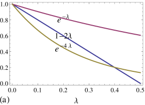
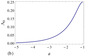
Figure 1: (Color online) (a) Graphical solution of Eq. (28) in terms of the convex function $\exp(2a\lambda)$ and the straight line $1-2\lambda$. As examples, $a=-0.5$ and $a=-2$ are used here to illustrate the shapes of the function $\exp(2a\lambda)$ for the two phases $a>-1$ and $a<-1$, respectively. (b) The discrete eigenvalue $\Lambda_{0}$ for $a<-1$. When $a=-1$, the discrete eigenvalue merges with the continuous spectrum $\Lambda\geq 1/4$.

For $\Lambda>1/4$, the eigenfunction can be obtained explicitly as [see Eqs. (59) and (63)]

$$u_{\Lambda}(v)=\left\{\begin{array}[]{lll}\sin(\kappa a)\sin(\kappa v)e^{-v/2}&&\\ \qquad+\kappa\sin[\kappa(v-a)]e^{-v/2}&&\mbox{for }v>0\\ \kappa\sin[\kappa(v-a)]e^{v/2}&&\mbox{for }a<v<0,\end{array}\right.$$ (34)

where $\kappa=\sqrt{\Lambda-1/4}>0$. Moreover, the normalization factor in Eq. (13) is given by [see Eq. (65)]

$$Z_{\Lambda}=\pi[\kappa^{2}+\kappa\sin(2a\kappa)+\sin^{2}(a\kappa)]/2,$$ (35)

and the integral over the eigenfunction which enters Eq. (14) is evaluated as

$$\int_{a}^{\infty}u_{\Lambda}(v)dv=\kappa^{2}e^{a/2}/(1/4+\kappa^{2}).$$ (36)

Thus, the spectrum consists of a continuous part $\Lambda>1/4$ and an additional discrete lowest eigenvalue $\Lambda_{0}$ for $a<-1$ which merges with the continuous spectrum at $a=-1$ [see Fig. 1(b)]. Hence we expect qualitative changes to appear at such a critical value.

By using Eqs. (4) and (14) we obtain the distribution of the FPT as follows

$$f(T,v_{0}) = \chi_{\{a\leq-1\}}\Lambda_{0}u_{\Lambda_{0}}(v_{0})e^{|v_{0}|-\Lambda_{0}T}\int_{a}^{\infty}u_{\Lambda_{0}}(v)dv/Z_{\Lambda_{0}}$$ (37)

$$+\frac{2}{\pi}e^{|v_{0}|-T/4+a/2}\int_{0}^{\infty}\kappa^{2}u_{\Lambda}(v_{0})e^{-\kappa^{2}T}/[\kappa^{2}+\kappa\sin(2a\kappa)+\sin^{2}(a\kappa)]d\kappa,$$

where $\chi_{\{a\leq-1\}}$ denotes the indicator function of the set $\{a\leq-1\}$, $u_{\Lambda_{0}}(v_{0})$ the eigenfunction of the discrete eigenvalue (27), and $u_{\Lambda}(v_{0})$ the eigenfunction of the continuous part of the spectrum (34). The normalizations $Z_{\Lambda_{0}}$ and $\int_{a}^{\infty}u_{\Lambda_{0}}(v)dv$ are given in Eqs. (29) and (30), respectively. In the trivial case $a=0$ the discontinuity does not enter the FPT problem and the pure dry friction model is equivalent to that of the one-dimensional Brownian motion with constant drift Kearney and Majumdar (2005). In such a case, the first term in Eq. (37) does not contribute and the integral can be evaluated in closed analytic form to yield

$$\!\!\!f(T,v_{0}) = \frac{2}{\pi}e^{v_{0}/2-T/4}\int_{0}^{\infty}\kappa\sin(\kappa v_{0})e^{-\kappa^{2}T}d\kappa$$ (38)

$$= \frac{1}{2\sqrt{\pi}}\frac{v_{0}}{T^{3/2}}e^{-(v_{0}-T)^{2}/(4T)}\quad\mbox{for }v_{0}>0,$$

a result which is consistent with Refs. Kearney and Majumdar (2005); Majumdar and Comtet (2002). Apart from this trivial case it seems to be difficult to obtain a closed analytic expression from the representation (37).

Certainly the FPT distribution changes qualitatively at $a=-1$ when the contribution in Eq. (37) coming from the discrete eigenvalue comes into play. That can be demonstrated by focussing on the tail behavior of the distribution which in itself is of interest when rare events are of interest. First of all it is obvious that for $a<-1$ the first term in Eq. (37) determines the decay which is plainly exponential $\exp(-\Lambda_{0}T)$. For $a\geq-1$, the first term in Eq. (37) vanishes, as the coefficient of the characteristic function vanishes at $a=-1$, and the tail is determined by evaluating the Laplace-type integral in the second term. If we have a closer look at the kernel entering the Laplace-type integral

$$\rho(\kappa,a)=\kappa^{2}u_{\Lambda}(v_{0})/[\kappa^{2}+\kappa\sin(2a\kappa)+\sin^{2}(a\kappa)],$$ (39)

it is evident that for $a>-1$ the properties

$$\lim_{\kappa\rightarrow 0}\rho(\kappa,a)=0,$$ (40)

$$\lim_{\kappa\rightarrow 0}\partial_{\kappa}\rho(\kappa,a)=0,$$ (41)

$$\lim_{\kappa\rightarrow 0}\partial_{\kappa}^{2}\rho(\kappa,a)\neq 0$$ (42)

hold (see Fig. 2). Hence it is straightforward to evaluate the Laplace-type integral to obtain a decay as $T^{-3/2}\exp(-T/4)$ for $a>-1$. For the critical case $a=-1$ the situation differs as

$$\lim_{\kappa\rightarrow 0}\rho(\kappa,-1)=\left\{\begin{array}[]{lll}1&&\mbox{for }v_{0}>0\\ 1+v_{0}&&\mbox{for }-1<v_{0}<0\end{array}\right.$$ (43)

holds. Here the Laplace method yields $T^{-1/2}\exp(-T/4)$ for $a=-1$. To summarize, in the long time limit we have

$$f(T,v_{0})\sim\left\{\begin{array}[]{lll}e^{-\Lambda_{0}T}&&\mbox{for }a<-1\\ T^{-1/2}e^{-T/4}&&\mbox{for }a=-1\\ T^{-3/2}e^{-T/4}&&\mbox{for }a>-1.\end{array}\right.$$ (44)

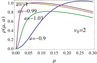
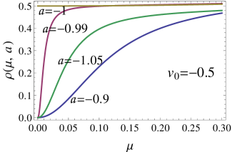
Figure 2: (Color online) The kernel $\rho(\kappa,a)$ [see Eq. (39)] appearing in the spectral decomposition (37) for two different values of $v_{0}$ and various values of the exit point $a$. Here $u_{\Lambda}(v_{0})$ is given by Eq. (34).

To obtain closed analytic expressions for the FPT distributions we alternatively can resort to the Laplace transform of the backward Kolmogorov equation. In this pure dry friction case Eq. (20) reads [see Eq. (26)]

$$\frac{\partial^{2}}{\partial v_{0}^{2}}\tilde{f}(s,v_{0})-\sigma(v_{0})\frac{\partial}{\partial v_{0}}\tilde{f}(s,v_{0})-s\tilde{f}(s,v_{0})=0,$$ (45)

where the solution has to satisfy the boundary conditions (21) and (22) as well as the matching condition (23) at $v_{0}=0$. It is in fact rather straightforward to compute the solution of this linear second order problem and we end up with

$$\tilde{f}(s,v_{0})=\left\{\begin{array}[]{lll}\exp\big{\{}[\sqrt{1+4s}(a-v_{0})+a+v_{0}]/2\big{\}}\sqrt{1+4s}/\theta(s,a)&&\mbox{for }v_{0}>0\\ \exp[(1+\sqrt{1+4s})(a-v_{0})/2]\theta(s,v_{0})/\theta(s,a)&&\mbox{for }a<v_{0}<0,\end{array}\right.$$ (46)

where we have introduced the abbreviation

$$\theta(s,a)=\exp\left(a\sqrt{1+4s}\right)+\sqrt{1+4s}-1$$ (47)

for the contribution appearing mainly in the denominator. Clearly Eq. (46) has a branch cut at $s=-1/4$ which relates with the continuous spectrum found previously. In addition, the condition $\theta(s,a)=0$, which is equivalent to Eq. (28), determines a pole for $a<-1$. Hence, when $a<-1$ the simple pole dominates the FPT distribution in the tail to yield an exponential decay Whitehouse et al. (2013). Overall, the analytical structure of the Laplace transform reflects the spectral properties mentioned previously.

The inverse Laplace transform of Eq. (46) does not seem to be available in closed analytic form. As before, only the trivial case $a=0$ can be handled with ease which then results in Eq. (38). For the other cases we resort to a so-called Talbot method Talbot (1979); Abate and Valkó (2004); Abate and Whitt (2006) to compute the FPT distribution in the time domain . Fig. 3 shows that the expressions (37) and (46) give identical results, as expected. In addition, evaluation of those expressions confirm as well the asymptotic decay given by Eq. (44) (see Fig. 4).

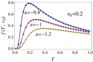
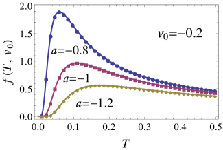
Figure 3: (Color online) The FPT distribution of the pure dry friction case [see Eq. (26)] for two values of initial velocity, $v_{0}=0.2$ and $v_{0}=-0.2$, and different escape ranges. Lines correspond to a numerical inversion of Eq. (46), and points to the evaluation of Eq. (37).

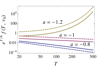
Figure 4: (Color online) Comparison of the FPT distribution obtained from Eq. (37) (solid) with the asymptotic result (44) (dashed) for the initial velocity $v_{0}=-0.2$ and different escape ranges. Data are plotted on a doubly logarithmic scale to uncover the power law corrections to the leading exponential behavior.

The closed form of the characteristic function (46) allows us to obtain easily the moments of the FPT via Eq. (24). For the first moment, i.e., for the mean first-passage time (MFPT) we have

$$\langle T\rangle=\left\{\begin{array}[]{lll}2e^{-a}+a+v_{0}-2&&\mbox{for }v_{0}>0\\ 2e^{-a}+a-v_{0}-2e^{-v_{0}}&&\mbox{for }a<v_{0}<0.\end{array}\right.$$ (48)

The first moment clearly displays a transition when the initial condition changes sign (see also Fig. 5). For $v_{0}>0$ the MFPT depends linearly on the initial velocity. No particular feature is visible at the transition at $a=-1$, as a change in the tail behavior has no impact on the low order moments of the distribution.

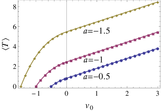
Figure 5: (Color online) The MFPT $\langle T\rangle$ for different escape ranges. Lines correspond to the analytic result (48), and points to a numerical evaluation of the first moment by using the spectral representation (37).

IV Biased Brownian motion with dry and viscous friction

In this section, we consider the full model (1) and set $\gamma=D=1$ without loss of generality. Other cases can be covered by using the appropriate rescaling

$$x=\left(\gamma/D\right)^{1/2}v,\qquad\tau=\gamma t.$$ (49)

Thus the model (1) can be written as Eq. (3) with

$$\Phi(v)=(|v|+\mu)^{2}/2-bv.$$ (50)

The corresponding eigenvalue problem (8) with potential (50) can be solved by using parabolic cylinder functions Buchholz (1969), which are denoted by $D_{\nu}(z)$. For the convenience of the reader we summarize the details of the derivation in Appendix B.

The eigenvalues are discrete and determined by the characteristic equation [see Eq. (78)]

$$\!\!\!\!\!\!\!\!\!\!\!\!\!\!\!\!\bar{\theta}(\Lambda,a,\mu,b)$$ (51)

$$= \Gamma(1-\Lambda)\{[D_{\Lambda}(\mu+b)D_{\Lambda-1}(\mu-b)$$

$$+D_{\Lambda}(\mu-b)D_{\Lambda-1}(\mu+b)]D_{\Lambda}(a-\mu-b)$$

$$-[D_{\Lambda}(-\mu-b)D_{\Lambda-1}(\mu-b)$$

$$-D_{\Lambda}(\mu-b)D_{\Lambda-1}(-\mu-b)]D_{\Lambda}(-a+\mu+b)\}$$

$$= 0.$$

For $\mu=0$, the model considered here reduces to the Ornstein-Uhlenbeck process and the characteristic equation (51) simply reads

$$D_{\Lambda}(a-b)=0,$$ (52)

which agrees with the standard result of the Ornstein-Uhlenbeck process (see for instance Ref. Siegert (1951)). It is furthermore unexpected that the characteristic equation (52) coincides with those of the odd part of the spectrum for a Fokker-Planck equation subjected to dry and viscous friction only Touchette et al. (2010). While odd eigenfunctions vanish at the origin and thus fulfil some kind of absorbing boundary condition it is not intuitively obvious why the argument of the parabolic cylinder function is in one case the absorbing boundary and in the other case the dry friction itself.

To link the current result with the previous section let us first consider the special case without bias ($b=0$). Intuitively, we expect that if the dry friction term dominates the viscous friction force then the particle will behave like the one subjected to dry friction only. Hence the spectrum obtained from Eq. (51) for large values of $\mu$ should resemble the spectrum described in the previous section [see, e.g., Fig. 1(b)]. In particular it means that a large gap should develop between the lowest eigenvalue and a quasicontinuous part for small negative values of $a$. For comparison of the models with and without viscous friction [see Eqs. (26) and (50)] we observe that a rescaling of the velocity by $\mu$ and of time by $\mu^{2}$ transforms the stochastic differential equation with dry and viscous friction to the model with dry friction and a small viscous part of $O(1/\mu^{2})$ which vanishes in the limit $\mu\rightarrow\infty$. Thus, to compare the eigenvalues obtained from the characteristic equation (51) with the spectrum computed in the previous section we rescale velocities by $\mu$ and eigenvalues by $1/\mu^{2}$. Then, indeed numerical evaluation of Eq. (51) confirms what one expects intuitively (see Fig. 6). The eigenvalues as a function of the exit position $a$ develop a gap if $\mu$ is sufficiently large, even though the transition is smoothened by the finite viscous friction. If dry and viscous friction become comparable, i.e., if $\mu$ becomes too small such a feature is going to disappear.

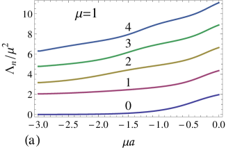
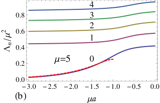
Figure 6: (Color online) The first five rescaled eigenvalues $\Lambda_{n}/\mu^{2}$ for the model without bias ($b=0$) as a function of the rescaled exit point $\mu a$ for two different values of $\mu$, according to Eq. (51). The dashed line in (b) depicts the discrete branch of the model with dry friction only [see Fig. 1(b)].

If we impose a force on the particle the finite bias will cause a stick-slip transition at $|b|=\mu$ where the minimum of the potential (50), i.e., the deterministic stationary state, changes from vanishing to finite velocity. The characteristics of such a transition are reflected by the eigenvalue spectrum as well (see Fig. 7). For small value of the bias, $|b|<\mu$, a case which we will call for brevity the dry phase, a substantial spectral gap appears between the lowest and the subleading eigenvalues. This gap shrinks when the transition at $|b|=\mu$ is approached. The spectral gap corresponds to a fast decay of velocity correlations in the system with small bias (see Ref. Touchette et al. (2010)). If the bias is sufficiently negative, i.e., $b<-\mu$, a case which we will call the wet phase, the potential (50) develops a quadratic minimum and the spectrum resembles that of the Ornstein-Uhlenbeck process. As with regards to the exit time problem a second transition will occur when on decreasing the force further the quadratic minimum of the potential moves beyond the exit point at $b=-\mu+a$. Then the exit from the region occurs in a purely ballistic way which decreases the exit time considerably. Hence that transition is related with an increase of the lowest eigenvalue (see Fig. 7). These two transitions are clearly visible if the diffusion is sufficiently small, i.e., $\mu$ sufficiently large. But they become obscured by noise for large diffusion, i.e., if $\mu$ becomes too small. Finally, in the dry phase the spectrum shows avoided level crossings for small bias, which are reminiscent of spectral properties in nonintegrable dynamical systems.

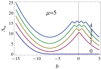
Figure 7: (Color online) The first five eigenvalues as a function of the bias $b$ for exit point at $a=-5$ and dry friction coefficient $\mu=5$, obtained from Eq. (51). The stick-slip transition, i.e., the narrowing of the spectral gap at $b=\pm\mu=\pm 5$ and the transition to a ballistic exit at $b=-\mu+a=-10$ are clearly visible.

As we have access to the entire spectrum we can derive from Eqs. (4) and (14) the FPT distribution

$$f(T,v_{0})=e^{\Phi(v_{0})}\sum_{\Lambda}\Lambda u_{\Lambda}(v_{0})e^{-\Lambda T}\int_{a}^{\infty}u_{\Lambda}(v)dv/Z_{\Lambda},$$ (53)

where the sum is taken over all the discrete eigenvalues [see Eq. (51)], $u_{\Lambda}(v_{0})$ refers to the eigenfunction given by Eq. (69), the integral $\int_{a}^{\infty}u_{\Lambda}(v)dv$ is stated in Eq. (79) and the normalization factor $Z_{\Lambda}$ is given by Eq. (82). It is thus straightforward to evaluate the shape of the distribution function (see, e.g., Fig. 8). While it seems to be difficult to obtain a closed analytic expression for this distribution we may pursue the approach used in the previous section and focus on the Laplace transform. In fact, Eq. (20) tells us that [see Eq. (50)]

$$\frac{\partial^{2}}{\partial v_{0}^{2}}\tilde{f}(s,v_{0})-(v_{0}+\mu\sigma(v_{0})-b)\frac{\partial}{\partial v_{0}}\tilde{f}(s,v_{0})-s\tilde{f}(s,v_{0})=0,$$ (54)

where the Laplace transform has to obey the boundary conditions (21) and (22) as well as the matching condition (23). Solving Eq. (54) is rather straightforward, as the boundary value problem for the Laplace transform is the formally adjoint of the eigenvalue problem [see Eqs. (67) and (68)]. It is well known and easy to confirm that the solution of the adjoint problem can be written in terms of the analytic expression for the eigenfunction (see Ref. Gardiner (1990)) if we multiply the eigenfunction with an exponential factor $\exp[\Phi(v_{0})]$ containing the potential (50). Thus, the solution of Eq. (54) can be written down directly as

$$\tilde{f}(s,v_{0})=\frac{e^{(a-\mu-b)^{2}/4-\Phi(a)}}{\bar{\theta}(-s,a,\mu,b)}u_{-s}(v_{0})e^{\Phi(v_{0})}\quad\mbox{for }v_{0}>a,$$ (55)

where $u_{-s}(v_{0})$ refers to Eq. (69), and the additional normalization factor containing the characteristic equation (51) is obtained by using the boundary condition (21). Obviously the poles of the Laplace transform are determined by the characteristic equation (51) and thus reflect the spectral structure discussed previously. In addition, the smallest simple pole determines the exponential tail of $f(T,v_{0})$.

As stated before, for $\mu=0$ the model investigated here corresponds to the exit time problem of the Ornstein-Uhlenbeck process, which has been paid much attention to in the past (see for instance Refs. Alili et al. (2006); Wang and Uhlenbeck (1945); Siegert (1951); Darling and Siegert (1953); Blake and Lindsey (1973); Leblanc and Scaillet (1998)). In this case Eq. (55) simplifies considerably and reads [see Eqs. (51) and (69)]

$$\tilde{f}(s,v_{0})=\frac{e^{(v_{0}-b)^{2}/4}D_{-s}(v_{0}-b)}{e^{(a-b)^{2}/4}D_{-s}(a-b)}\quad\mbox{for }v_{0}>a,$$ (56)

which is consistent with the standard result stated, for instance, in Ref. Siegert (1951).

The analytic expressions Eqs. (53) or (55) now allow us to discuss the dependence of the exit time problem on the initial velocity $v_{0}$. Both expressions, if properly evaluated, give of course identical results (see Fig. 8). Here we are going to pay particular attention to the impact of the discontinuity appearing at the origin. Depending on the sign of the initial velocity the particle has to pass the discontinuity at $v=0$ before exiting at $a<0$. Thus, a qualitative change of the FPT distribution is expected depending on the sign of $v_{0}$. In fact, such a feature is already visible from Eq. (55), as different analytical branches of the eigenfunction (69) come into play if $v_{0}$ changes sign. The dependence on $v_{0}$ is still smooth but not differentiable of higher order. The FPT distributions for small positive and small negative values of $v_{0}$ look distinctively different, as shown in Fig. 8. For $v_{0}>0$ the particle has to pass through $v=0$ before exiting and thus sticks at the origin at least if the bias is small, causing larger exit times. Thus, the distribution overall is shifted to the right, compared to the case $v_{0}<0$.

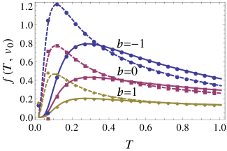
Figure 8: (Color online) The distribution of the FPT for $\mu=1$, $a=-1$, two values of initial velocity, $v_{0}=0.2$ (solid) and $v_{0}=-0.2$ (dashed), and different values of the bias $b$. Lines correspond to a numerical inversion of the Laplace transform (55), and points to the evaluation of Eq. (53) taking the first twenty modes into account. A larger number of modes would be required to reproduce the exact result for very small values of $t$.

The just mentioned phenomenon can be better illustrated by looking at the MFPT which can be obtained in closed analytic form via Eqs. (24) and (55) even for very small values of the diffusion, i.e., for large values of $\mu$. While the analytic expression can be written down we just refer to the graphical evaluation of the expressions (see Fig. 9). For small bias, $|b|<\mu$, i.e., in the dry phase there is a possibility that the particle sticks at the origin which will impact on the MFPT. If the particle starts at $v_{0}<0$ it has less chance to stick at the origin when $v_{0}$ becomes smaller, and the change of the MFPT with regards to $v_{0}$ becomes fairly large. On the contrary, if we choose a positive initial velocity $v_{0}>0$, the particle has always to pass $v=0$ before exiting at $a<0$. Thus no huge variation of the MFPT with $v_{0}$ is detected. If we decrease the bias and enter the wet phase $b<-\mu$, the particle does not stick any more and the just mentioned feature almost disappears. This scenario is much more pronounced if we look at the first derivative $\partial_{v_{0}}\langle T\rangle$ [see Fig. 9(b)]. Like the distribution function itself the MFPT is continuously differentiable, but loses analyticity due to the discontinuity at $v_{0}=0$. A kink can be seen clearly at the origin for small bias $|b|<\mu$, which separates the two different regimes of the MFPT for negative and positive initial velocities. This feature is suppressed if we decrease the bias and finally enter the wet phase with $b<-\mu$ where the kink almost disappears.

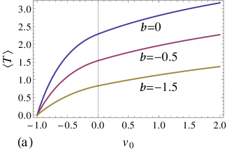
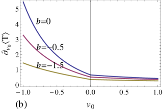
Figure 9: (Color online) (a) MFPT $\langle T\rangle$ as a function of the initial value $v_{0}$ for $\mu=1$, exit condition $a=-1$, and different values of the bias, covering the dry phase $|b|<\mu$ as well as the wet phase $b<-\mu$. (b) First derivative of the MFPT with respect to the initial value for the same data.

V Conclusion

In this paper we have studied the FPT problem of Brownian motion with dry and viscous friction. There has been renewed interest in such exit time problems from two different points of view. On the one hand prediction and forecasting of extreme events and the related large deviation theory are closely related to exit time problems. On the other hand, the particular setup studied here is a special example of a piecewise-smooth dynamical system. While such systems are extensively used in engineering sciences only recently the attempt has been made to put this subject in the systematic framework of dynamical system’s theory.

As a case study we have considered here a simple piecewise-linear model which can be largely solved by analytical means. In physicists terms we have considered a particle subjected to dry and viscous friction, to noise, and to an external force. This is one of the few models for which the FPT distribution can be obtained analytically either by solving the Fokker-Planck equation via a spectral decomposition method or by solving the backward Kolmogorov equation in the Laplace space. While the first method gives more insight into the underlying dynamical mechanisms through the additional spectral information, the second is able to deliver closed analytic expressions for the MFPT.

The simplest case, where only dry friction acts on the particle, already shows one of the main features, a phase transition phenomenon in the spectrum which is related to the position of the exit point. A unique discrete eigenvalue links up with the continuous part of the spectrum at a critical size of the exit region. Such a transition translates into different asymptotic properties of the FPT distribution. The signature of this transition persists if the viscous friction and the external bias are taken into account, even though the transition is blurred by the finite diffusion. In this full model two new features occur, i.e., a stick-slip transition and a transition to a ballistic exit of the particle. All three transitions are clearly visible in the discrete spectrum of the full model, especially at low diffusion, signalling the different rates of asymptotic decay of the FPT distribution. As an aside, the analysis of this model covers as special cases the Ornstein-Uhlenbeck process on the one hand, and the previously discussed dry friction case on the other.

The availability of analytical results for higher dimensional stochastic models is rather limited, contrary to the one-variable case. Even the computation of the stationary distribution is often a challenge if detailed balance is violated, and dynamical quantities, like correlations or exit probabilities are certainly out of reach. Having said that, models with more than one degree of freedom are prevalent in applications and any progress on the analytical side is certainly welcomed, even if simple model systems are considered. In that sense the inclusion of inertia in the model discussed here is a rewarding goal, which could lead to predictions that are experimentally relevant and could trigger corresponding experimental investigations. Progress in that direction seems possible even though the analysis may not be entirely straightforward.

Appendix A Eigenvalue problem for the inviscid case

Without viscous damping and driving Eq. (8) reads [see Eq. (26)]

$$-\Lambda u_{\Lambda}(v)=u_{\Lambda}^{\prime}(v)+u_{\Lambda}^{\prime\prime}(v) \quad\mbox{for }v>0$$ (57)

$$-\Lambda u_{\Lambda}(v)=-u_{\Lambda}^{\prime}(v)+u_{\Lambda}^{\prime\prime}(v) \quad\mbox{for }a<v<0.$$ (58)

Let

$$u_{\Lambda}(v)=e^{-|v|/2}\varphi_{\Lambda}(v),$$ (59)

then Eqs. (57) and (58) can be written as

$$\varphi^{\prime\prime}_{\Lambda}(v)=(1/4-\Lambda)\varphi_{\Lambda}(v)\quad\mbox{for }v\neq 0.$$ (60)

On the one hand, for $\Lambda<1/4$ let us introduce the positive variable $\lambda=\sqrt{1/4-\Lambda}$. Then the solution of Eq. (60) which results in a finite normalization factor [see Eq. (12)] is given by

$$\varphi_{\Lambda}(v)=\left\{\begin{array}[]{lll}A_{\lambda}e^{-\lambda v}&&\mbox{for }v>0\\ B_{\lambda}e^{\lambda v}+C_{\lambda}e^{-\lambda v}&&\mbox{for }a<v<0.\end{array}\right.$$ (61)

Choose $A_{\lambda}=2\lambda$ and use the matching conditions (10) and (11) to determine the other two coefficients in Eq. (61) as

$$B_{\lambda}=1,\qquad C_{\lambda}=2\lambda-1.$$ (62)

The eigenvalue is now determined by the absorbing boundary condition (9), i.e., $\varphi_{\Lambda}(a)=0$, which results in Eq. (28).

On the other hand, for $\Lambda>1/4$ the solution of Eq. (60) which vanishes at $v=a$, i.e., which satisfies the absorbing boundary condition (9), is given by

$$\varphi_{\Lambda}(v)=\left\{\begin{array}[]{lll}\bar{A}_{\kappa}\sin(\kappa v)+\bar{B}_{\kappa}\cos(\kappa v)&&\mbox{for }v>0\\ \bar{C}_{\kappa}\kappa\sin[\kappa(v-a)]&&\mbox{for }a<v<0,\end{array}\right.$$ (63)

where we have introduced the abbreviation $\kappa=\sqrt{\Lambda-1/4}>0$. Choose $\bar{C}_{\kappa}=\kappa$, then by using the matching conditions (10) and (11), the two parameters $\bar{A}_{\kappa}$ and $\bar{B}_{\kappa}$ are evaluated as

$$\bar{A}_{\kappa}=\kappa\cos(a\kappa)+\sin(a\kappa),\qquad\bar{B}_{\kappa}=-\kappa\sin(a\kappa).$$ (64)

Hence Eq. (34) follows from substituting Eq. (63) into Eq. (59). For the normalization, Eqs. (59) and (63) result in

$$\!\!\!\!\!\!\!\!\!\!\!\!\!\!\!\!\!\!\!\!\!\int_{a}^{\infty}u_{\Lambda}(v)u_{\Lambda^{\prime}}(v)e^{|v|}dv$$ (65)

$$= \int_{0}^{\infty}[\bar{A}_{\kappa}\sin(\kappa v)+\bar{B}_{\kappa}\cos(\kappa v)][\bar{A}_{\kappa^{\prime}}\sin(\kappa^{\prime}v)+\bar{B}_{\kappa^{\prime}}\cos(\kappa^{\prime}v)]dv+\int_{a}^{0}\kappa\kappa^{\prime}\sin[\kappa(v-a)]\sin[\kappa^{\prime}(v-a)]dv$$

$$= \int_{0}^{\infty}\bigg{\{}\frac{1}{2}\big{(}\bar{A}_{\kappa}\bar{A}_{\kappa^{\prime}}+\bar{B}_{\kappa}\bar{B}_{\kappa^{\prime}}\big{)}\cos[(\kappa-\kappa^{\prime})v]+\frac{1}{2}\big{(}\bar{B}_{\kappa}\bar{B}_{\kappa^{\prime}}-\bar{A}_{\kappa}\bar{A}_{\kappa^{\prime}}\big{)}\cos[(\kappa+\kappa^{\prime})v]$$

$$+\frac{1}{2}\big{(}\bar{A}_{\kappa}\bar{B}_{\kappa^{\prime}}-\bar{A}_{\kappa^{\prime}}\bar{B}_{\kappa}\big{)}\sin[(\kappa-\kappa^{\prime})v]+\frac{1}{2}\big{(}\bar{A}_{\kappa}\bar{B}_{\kappa^{\prime}}+\bar{A}_{\kappa^{\prime}}\bar{B}_{\kappa}\big{)}\sin[(\kappa+\kappa^{\prime})v]\bigg{\}}dv-\frac{\kappa\bar{A}_{\kappa}\bar{B}_{\kappa^{\prime}}-\kappa^{\prime}\bar{A}_{\kappa^{\prime}}\bar{B}_{\kappa}}{\kappa^{2}-{\kappa^{\prime}}^{2}}$$

$$= \frac{\pi}{2}(\bar{A}_{\kappa}^{2}+\bar{B}_{\kappa}^{2})\delta(\kappa-\kappa^{\prime}),$$

which shows that the normalization factor $Z_{\Lambda}$ satisfies Eq. (35) if we take Eq. (64) into account. To derive Eq. (65), we have used the standard identities for the $\delta$– and the principal value distribution

$$\int_{0}^{\infty}\cos(\kappa v)dv=\pi\delta(\kappa),\qquad\int_{0}^{\infty}\sin(\kappa v)dv=P\left(\frac{1}{\kappa}\right).$$ (66)

Appendix B Eigenvalue problem for the general case

For the model (1), the eigenvalue problem (8) reads

$$-\Lambda u_{\Lambda}(v)=[(v+\mu-b)u_{\Lambda}(v)]^{\prime}+u_{\Lambda}^{\prime\prime}(v) \mbox{ for }v>0$$ (67)

$$-\Lambda u_{\Lambda}(v)=[(v-\mu-b)u_{\Lambda}(v)]^{\prime}+u_{\Lambda}^{\prime\prime}(v) \mbox{ for }a<v<0,$$ (68)

if we adopt the notation used for Eq. (50). These two equations are a special case of the so-called Kummer’s equation, which can be solved in terms of parabolic cylinder functions Touchette et al. (2010). The solution of Eqs. (67) and (68) which vanishes at infinity is given by (see Refs. Touchette et al. (2012); Buchholz (1969))

$$u_{\Lambda}(v)=\left\{\begin{array}[]{lll}A_{\Lambda}e^{-(v+\mu-b)^{2}/4}D_{\Lambda}(v+\mu-b)&&\mbox{for }v>0\\ B_{\Lambda}e^{-(v-\mu-b)^{2}/4}D_{\Lambda}(v-\mu-b)+C_{\Lambda}e^{-(v-\mu-b)^{2}/4}D_{\Lambda}(-v+\mu+b)&&\mbox{for }a<v<0,\end{array}\right.$$ (69)

where $D_{\Lambda}$ denotes the parabolic cylinder function. Here we have used a fundamental system in terms of $D_{\nu}(z)$ and $D_{\nu}(-z)$ to write down the solution. Such a fundamental system degenerates for $\nu$ being an integer. Thus, our expressions may contain spurious singularities at integer values of $\Lambda$ which have to be taken care of. The coefficients $A_{\Lambda}$, $B_{\Lambda}$ and $C_{\Lambda}$ depend on the parameters $b$ and $\mu$ as well, but are independent of $v$.

Using Eq. (69) the matching conditions (10) and (11) result in a set of linear homogeneous equations

$$B_{\Lambda}D_{\Lambda}(-\mu-b)+C_{\Lambda}D_{\Lambda}(\mu+b)=e^{\mu b}A_{\Lambda}D_{\Lambda}(\mu-b),$$ (70)

$$B_{\Lambda}D_{1+\Lambda}(-\mu-b)-C_{\Lambda}D_{1+\Lambda}(\mu+b)=e^{\mu b}A_{\Lambda}[D_{1+\Lambda}(\mu-b)-2\mu D_{\Lambda}(\mu-b)]$$ (71)

when the property

$$\frac{de^{-z^{2}/4}D_{\nu}(z)}{dz}=-e^{-z^{2}/4}D_{\nu+1}(z)$$ (72)

of the parabolic cylinder function is employed. For $A_{\Lambda}$ we choose

$$A_{\Lambda}=\sqrt{2\pi}e^{-\mu b}.$$ (73)

Then, the other two coefficients in Eq. (69) follow as

$$B_{\Lambda} = -\Lambda\Gamma(-\Lambda)[D_{\Lambda}(\mu+b)D_{\Lambda-1}(\mu-b)$$ (74)

$$+D_{\Lambda}(\mu-b)D_{\Lambda-1}(\mu+b)],$$

$$C_{\Lambda} = \Lambda\Gamma(-\Lambda)[D_{\Lambda}(-\mu-b)D_{\Lambda-1}(\mu-b)$$ (75)

$$-D_{\Lambda}(\mu-b)D_{\Lambda-1}(-\mu-b)],$$

where we have used the identities

$$D_{\nu}(z)D_{\nu+1}(-z)+D_{\nu}(-z)D_{\nu+1}(z)=\frac{\sqrt{2\pi}}{\Gamma(-\nu)},$$ (76)

$$zD_{\nu}(z)-D_{\nu+1}(z)-\nu D_{\nu-1}(z)=0$$ (77)

to simplify the above two expressions.

The characteristic equation simply follows from the boundary condition (9), and is thus given by

$$B_{\Lambda}D_{\Lambda}(a-\mu-b)+C_{\Lambda}D_{\Lambda}(-a+\mu+b)=0.$$ (78)

Using the identities (76) and (77) we arrive at Eq. (51).

For the integral over the eigenfunction which enters the FPT distribution (53) we obtain by using, e.g., the differential identity (72)

$$\int_{a}^{\infty}u_{\Lambda}(v)dv = A_{\Lambda}e^{-(\mu-b)^{2}/4}D_{\Lambda-1}(\mu-b)-e^{-(\mu+b)^{2}/4}[B_{\Lambda}D_{\Lambda-1}(-\mu-b)-C_{\Lambda}D_{\Lambda-1}(\mu+b)]$$ (79)

$$+e^{-(a-\mu-b)^{2}/4}[B_{\Lambda}D_{\Lambda-1}(a-\mu-b)-C_{\Lambda}D_{\Lambda-1}(-a+\mu+b)].$$

Finally to compute the normalization let us consider the integral

$$\!\!\!\!\!\!\!\!\!\!\!\!\!\!\!\!\!\!\!\!\!(\Lambda-\Lambda^{\prime})\int_{a}^{\infty}e^{(v+\mu\sigma(v))^{2}/2-bv}u_{\Lambda}(v)u_{\Lambda^{\prime}}(v)dv$$ (80)

$$= e^{-\mu b-b^{2}/2}(\Lambda-\Lambda^{\prime})\int_{a}^{0}[B_{\Lambda}D_{\Lambda}(v-\mu-b)+C_{\Lambda}D_{\Lambda}(-v+\mu+b)]$$

$$\times[B_{\Lambda^{\prime}}D_{\Lambda^{\prime}}(v-\mu-b)+C_{\Lambda^{\prime}}D_{\Lambda^{\prime}}(-v+\mu+b)]dv$$

$$+e^{\mu b-b^{2}/2}(\Lambda-\Lambda^{\prime})A_{\Lambda}A_{\Lambda^{\prime}}\int_{0}^{\infty}D_{\Lambda}(v+\mu-b)D_{\Lambda^{\prime}}(v+\mu-b)dv$$

$$= e^{-\mu b-b^{2}/2}(\Lambda-\Lambda^{\prime})\int_{a-\mu-b}^{-\mu-b}[B_{\Lambda}D_{\Lambda}(v)+C_{\Lambda}D_{\Lambda}(-v)][B_{\Lambda^{\prime}}D_{\Lambda^{\prime}}(v)+C_{\Lambda^{\prime}}D_{\Lambda^{\prime}}(-v)]dv$$

$$+e^{\mu b-b^{2}/2}(\Lambda-\Lambda^{\prime})A_{\Lambda}A_{\Lambda^{\prime}}\int_{\mu-b}^{\infty}D_{\Lambda}(v)D_{\Lambda^{\prime}}(v)dv$$

$$= e^{-\mu b-b^{2}/2}\big{\{}-B_{\Lambda}D_{\Lambda+1}(a-\mu-b)[B_{\Lambda^{\prime}}D_{\Lambda^{\prime}}(a-\mu-b)+C_{\Lambda^{\prime}}D_{\Lambda^{\prime}}(\mu-a+b)]$$

$$+B_{\Lambda^{\prime}}D_{\Lambda^{\prime}+1}(a-\mu-b)[B_{\Lambda}D_{\Lambda}(a-\mu-b)+C_{\Lambda}D_{\Lambda}(\mu-a+b)]$$

$$+C_{\Lambda}D_{\Lambda+1}(\mu-a+b)[B_{\Lambda^{\prime}}D_{\Lambda^{\prime}}(a-\mu-b)+C_{\Lambda^{\prime}}D_{\Lambda^{\prime}}(\mu-a+b)]$$

$$-C_{\Lambda^{\prime}}D_{\Lambda^{\prime}+1}(\mu-a+b)[B_{\Lambda}D_{\Lambda}(a-\mu-b)+C_{\Lambda}D_{\Lambda}(\mu-a+b)]\big{\}}.$$

For the last computational step we have used the properties (72) and the analogous identity

$$\frac{de^{z^{2}/4}D_{\nu}(z)}{dz}=\nu e^{z^{2}/4}D_{\nu-1}(z).$$ (81)

Indeed, if we choose for $\Lambda$ and $\Lambda^{\prime}$ two different eigenvalues we obtain (bi-)orthogonality of the eigenfunctions if the characteristic equation (78) is taken into account. Furthermore dividing Eq. (80) on both sides by $\Lambda-\Lambda^{\prime}$ and taking the limit $\Lambda^{\prime}\rightarrow\Lambda$ we end up with the normalization factor

$$Z_{\Lambda}=e^{-\mu b-b^{2}/2}\left[B_{\Lambda}D_{\Lambda+1}(a-\mu-b)-C_{\Lambda}D_{\Lambda+1}(\mu-a+b)\right]\partial_{\Lambda}\left[B_{\Lambda}D_{\Lambda}(a-\mu-b)+C_{\Lambda}D_{\Lambda}(\mu-a+b)\right].$$ (82)

References

- Kramers (1940) H. A. Kramers, Physica 7, 284 (1940).
- Hänggi et al. (1990) P. Hänggi, P. Talkner, and M. Borkovec, Rev. Mod. Phys. 62, 251 (1990).
- Mannella (2004) R. Mannella, J. Comput. Finance 7, 1 (2004).
- Tuckwell et al. (2002) H. C. Tuckwell, F. Y. M. Wan, and J. P. Rospars, Biol. Cybernet. 86, 137 (2002).
- Condamin et al. (2007) S. Condamin, O. Bénichou, V. Tejedor, R. Voituriez, and J. Klafter, Nature 450, 77 (2007).
- Redner (2001) S. Redner, A guide to first-passage processes (Cambridge University Press, Cambridge, 2001).
- Bray et al. (2013) A. J. Bray, S. N. Majumdar, and G. Schehr, Adv. Phys. 62, 225 (2013).
- Majumdar (2005) S. N. Majumdar, Current Science 89, 2076 (2005).
- Kearney and Majumdar (2005) M. J. Kearney and S. N. Majumdar, J. Phys. A: Math. Gen. 38, 4097 (2005).
- Siegert (1951) A. J. F. Siegert, Phys. Rev. 81, 617 (1951).
- Alili et al. (2006) L. Alili, P. Patie, and J. L. Pedersen, Stoch. Models 21, 967 (2006).
- Göing-Jaeschke and Yor (2003) A. Göing-Jaeschke and M. Yor, Bernoulli 9, 313 (2003).
- DeBlassie and Smits (2007) D. DeBlassie and R. Smits, Stoch. Proc. Appl. 117, 629 (2007).
- Makarenkov and Lamb (2012) O. Makarenkov and J. S. W. Lamb, Physica D 241, 1826 (2012).
- Vanossi et al. (2013) A. Vanossi, N. Manini, M. Urbakh, S. Zapperi, and E. Tosatti, Rev. Mod. Phys. 85, 529 (2013).
- Karatzas and Shreve (1984) I. Karatzas and S. E. Shreve, Ann. Prob. 12, 819 (1984).
- Touchette et al. (2010) H. Touchette, E. V. der Straeten, and W. Just, J. Phys. A: Math. Theor. 43, 445002 (2010).
- Touchette et al. (2012) H. Touchette, T. Prellberg, and W. Just, J. Phys. A: Math. Theor. 45, 395002 (2012).
- Simpson and Kuske (2012) D. J. W. Simpson and R. Kuske, arXiv:1204.5792 (2012).
- de Gennes (2005) P.-G. de Gennes, J. Stat. Phys. 119, 953 (2005).
- Hayakawa (2005) H. Hayakawa, Physica D 205, 48 (2005).
- Karatzas and Shreve (1991) I. Karatzas and S. E. Shreve, Brownian motion and stochastic calculus (Springer, Berlin, 1991).
- Baule et al. (2010) A. Baule, E. G. D. Cohen, and H. Touchette, J. Phys. A: Math. Theor. 43, 025003 (2010).
- Baule et al. (2011) A. Baule, H. Touchette, and E. G. D. Cohen, Nonlinearity 24, 351 (2011).
- Chen et al. (2013) Y. Chen, A. Baule, H. Touchette, and W. Just, Phys. Rev. E 88, 052103 (2013).
- Chaudhury and Mettu (2008) M. K. Chaudhury and S. Mettu, Langmuir 24, 6128 (2008).
- Goohpattader et al. (2009) P. S. Goohpattader, S. Mettu, and M. K. Chaudhury, Langmuir 25, 9969 (2009).
- Gnoli et al. (2013) A. Gnoli, A. Puglisi, and H. Touchette, Europhys. Lett. 102, 14002 (2013).
- Goohpattader and Chaudhury (2010) P. S. Goohpattader and M. K. Chaudhury, J. Chem. Phys. 133, 024702 (2010).
- Wang and Uhlenbeck (1945) M. C. Wang and G. E. Uhlenbeck, Rev. Mod. Phys. 17, 323 (1945).
- Risken (1989) H. Risken, The Fokker-Planck equation: methods of solution and applications (Springer, Berlin, 1989).
- Gardiner (1990) C. W. Gardiner, Handbook of stochastic methods for physics, chemistry and the natural sciences (Springer, Berlin, 1990).
- Horsthemke and Lefever (1984) W. Horsthemke and R. Lefever, Noise-induced transitions (Springer, Berlin, 1984).
- Wong (1964) E. Wong, The construction of a class of stationary Markoff processes, Stochastic Processes in Mathematical Physics and Engineering (Providence, R.I.: American Mathematical Society, 1964).
- Corless et al. (1996) R. M. Corless, G. H. Gonnet, D. E. G. Hare, D. J. Jeffrey, and D. E. Knuth, Adv. Comp. Math. 5, 329 (1996).
- Majumdar and Comtet (2002) S. N. Majumdar and A. Comtet, Phys. Rev. E 66, 061105 (2002).
- Whitehouse et al. (2013) J. Whitehouse, M. R. Evans, and S. N. Majumdar, Phys. Rev. E 87, 022118 (2013).
- Talbot (1979) A. Talbot, IMA J. Appl. Math. 23, 97 (1979).
- Abate and Valkó (2004) J. Abate and P. P. Valkó, Int. J. Numer. Methods 60, 979–993 (2004).
- Abate and Whitt (2006) J. Abate and W. Whitt, INFORMS J. Comput. 18, 408–421 (2006).
- Buchholz (1969) H. Buchholz, The confluent hypergeometric function with spectial emphasis on its applications (Springer, Berlin, 1969).
- Darling and Siegert (1953) D. A. Darling and A. J. F. Siegert, Annals of Math. Statist. 24, 624 (1953).
- Blake and Lindsey (1973) I. F. Blake and W. C. Lindsey, IEEE Trans. Inform. Theory IT-19, 295 (1973).
- Leblanc and Scaillet (1998) B. Leblanc and O. Scaillet, Finance Stochast. 2, 349 (1998).