SpeedMachines: Anytime Structured Prediction

Abstract

Structured prediction plays a central role in machine learning applications from computational biology to computer vision. These models require significantly more computation than unstructured models, and, in many applications, algorithms may need to make predictions within a computational budget or in an anytime fashion. In this work we propose an anytime technique for learning structured prediction that, at training time, incorporates both structural elements and feature computation trade-offs that affect test-time inference. We apply our technique to the challenging problem of scene understanding in computer vision and demonstrate efficient and anytime predictions that gradually improve towards state-of-the-art classification performance as the allotted time increases.

1 Introduction

In real-world applications, we are often forced to trade-off between accurate predictions and the computation time needed to make them. In many problems, structured prediction algorithms are necessary to obtain accurate predictions; however, this class of techniques is typically more computationally demanding over simpler locally independent predictions. Furthermore, under limited computational resources we may forced to make a prediction after a limited and unknown amount of time. Therefore, we require an approach that is efficient while also capable of returning a sensible prediction when requested at any time. Furthermore, as the inference procedure is given more time, we should expect the predictive performance to also increase.

The contribution of this work is an algorithm for making anytime structured predictions. As detailed in the following sections, our approach accounts for both inference and feature computation times while automatically trading-off cost for accuracy, and vice versa, in order to maximize predictive performance with respect to computation time. Although our approach is applicable towards a variety of different structured prediction problems, we analyze its efficacy on the challenging problem of scene understanding in computer vision. Our experiments demonstrate that we can learn an efficient, anytime predictor whose classification performance improves towards state-of-the-art while automatically selecting what features to compute and where to compute them with respect to time.

1.1 Related Work

A canonical approach for incorporating computation time during learning is a cascade of feed-forward modules, where each module becomes more sophisticated but also more computationally expensive the further it is down the cascade [26]. One drawback of the cascade approach is that the procedure is trained for a specific sequence length and is not suited for interruption. For example, stopping predictions after one module in a long cascade will generally perform much worse than a predictor that was trained in isolation. Recent works [9, 12, 29, 14] have investigated techniques for learning locally independent predictors which balance feature computation time and inference time during learning; however, they are not immediately amenable to the structured prediction scenario.

In the structured setting, Jiang et al. [13] proposed a technique for reinforcement learning that incorporates a user specified speed/accuracy trade-off distribution, and Weiss and Taskar [27] proposed a cascaded analog for structured prediction where the solution space is is iteratively refined/pruned over time. In contrast, we are focused on learning a structured predictor with interruptible, anytime properties which is also trained to balance both the structural and feature computation times during the inference procedure. Recent work in computer vision and robotics [23, 5] has similarly investigated techniques for making approximate inference in graphical models more efficient via a cascaded procedure that iteratively prunes subregions in the scene to analyze. We similarly incorporate such structure selection in our approach; however, we also account for feature computation time and avoid the early hard commitments required with a cascaded approach. This allows for early predictions to be as accurate as possible, as they do not have to be made conservatively as in the cascade approach.

2 Background

2.1 Structured Prediction

In the structured prediction setting, we are given inputs $x\in\mathcal{X}$ and associated structured outputs $y\in\mathcal{Y}$. The goal is to learn a function $f:\mathcal{X}\rightarrow\mathcal{Y}$ that minimizes some risk ${\mathcal{R}}[f]$, typically evaluated pointwise over the inputs:

$${\mathcal{R}}[f]=\mathbb{E}_{\mathcal{X}}[l(f(x))].$$ (1)

We will further assume that each input and output pair has some underlying structure, such as the graph structure of graphical models, that can be utilized to predict portions of the output locally. Let $j$ index these structural elements. We then assume that a final structured output $y$ can be represented as a variable length vector $(y_{1},\ldots,y_{J})$, where each element $y_{j}$ lies in some vector space $y_{j}\in\mathcal{Y}^{\prime}$. For example, these outputs could be the probability distribution over class labels for each pixel in an image, or distributions of part-of-speech labels for each word in a sentence. Similarly we can compute some features $x_{j}$ representing the portion of the input which corresponds to a given output, such as features computed over a neighborhood around a pixel in an input image.

As another example, consider labeling tasks such as part-of-speech tagging. In this domain, we are given a set of input sentences $\mathcal{X}$, and for each word $j$ in a given sentence, we want to output a vector $\hat{y}_{j}\in\mathbb{R}^{K}$ containing the scores with respect to each of the $K$ possible part-of-speech labels for that word. This sequence of vectors for each word is the complete structured prediction $\hat{y}$. An example loss function for this domain would be the multiclass log-loss, averaged over words, with respect to the ground truth parts-of-speech.

Along with the encoding of the problem, we also assume that the structure can be used to reduce the scope of the prediction problem, as in graphical models. One common approach to generating predictions on these structures is to use a policy-based or iterative decoding approach, instead of probabilistic inference over a graphical model [3, 4, 25, 21, 20]. In order to model the contextual relationships among the outputs, these iterative approaches commonly perform a sequence of predictions, where each update relies on previous predictions made across the structure of the problem.

Let $N(j)$ represent the locally connected elements of $j$, such as the locally connected factors of a node $j$ in a typical graphical model. For a given node $j$, the predictions over the neighboring nodes $\hat{y}_{N(j)}$ can then be used to update the prediction for that node. For example, in the character recognition task, the predictions for neighboring characters can influence the prediction for a given character, and be used to update and improve the accuracy of that prediction.

In the iterative decoding approach a predictor $\phi$ is iteratively used to update different elements $\hat{y}_{j}$ of the final structured output:

$$\hat{y}_{j}=\phi(x_{j},\hat{y}_{N(j)}).$$ (2)

A complete policy then consists of a strategy for selecting which elements of the structured output to update, coupled with the predictor for updating the given outputs. Typical approaches include randomly selecting elements to update, iterating over the structure in a fixed ordering, or simultaneously updating all predictions at all iterations. As shown by Ross et al. [20], this iterative decoding approach can is equivalent to message passing approaches used to solve graphical models, where each update encodes a single set of messages passed to one node in the graphical model.

2.2 Anytime Prediction

In traditional boosting, the goal is to learn a function

$$f(x)=\sum_{t}\alpha_{t}h_{t}(x),$$ (3)

which is additively built from a set of weaker predictors $h\in\mathcal{H}$ that minimizes some risk functional $\operatorname*{arg\,min}_{f\in\mathcal{F}}{\mathcal{R}}[f]$. Minimizing this functional can be viewed as performing gradient descent in function space [18, 8]. Assuming the loss function is of the form given in (Eq. 1), the functional gradient, $\nabla=\nabla_{f}{\mathcal{R}}[f]$, is a function of the form

$$\nabla(x)=\frac{\partial l(f(x))}{\partial f(x)}.$$ (4)

The weak predictor $h$ that best minimizes the projection error of the functional gradient is selected at each iteration:

$$h_{t} =\operatorname*{arg\,max}_{h\in\mathcal{H}}{\left\langle{\nabla{\mathcal{R}}[f_{t-1}]},{h}\right\rangle},$$ (5)

$$\alpha_{t} =\operatorname*{arg\,min}_{\alpha\in\mathbb{R}}{\mathcal{R}}[f_{t-1}+\alpha h_{t}].$$ (6)

Minimizing this projection error can be equivalently performed through the least squares minimization

$$h_{t}=\operatorname*{arg\,min}_{h\in\mathcal{H}}\mathbb{E}_{\mathcal{X}}\left[\|\nabla(x)-h(x)\|^{2}\right].$$ (7)

Extending this framework, Grubb and Bagnell [12] introduce an anytime prediction method that modifies the standard boosting criterion to automatically trade-off the loss of a weak predictor, $h$, with its cost $c(h)\in\mathbb{R}^{+}$. They do this by using a cost-greedy selection criterion that selects the weak predictor which gets the best improvement in loss per unit cost,

$$h_{t},\alpha_{t}=\operatorname*{arg\,max}_{h\in\mathcal{H},\alpha\in\mathbb{R}}\frac{\mathcal{R}\left[f_{t-1}\right]-\mathcal{R}\left[f_{t-1}+\alpha h\right]}{c(h)}.$$ (8)

Hence, for some fixed number of iterations $T$, the total cost of the learned function is $c(f_{T})=\sum_{t=1}^{T}c(h_{t})$. The learned predictor can easily adjust to any new budget of costs by evaluating the sequence until the budget is exhausted. Grubb and Bagnell prove that this SpeedBoost algorithm updates the resulting predictions at an increasing sequence of budgets that is competitive with any other sequence which uses the same weak predictors for a wide range of budgets [12].

3 Anytime Structured Prediction

3.1 Weak Structured Predictors

We adapt the SpeedBoost framework to the structured prediction setting by learning an additive structured predictor. To accomplish this, we will adapt the policy-based iterative decoding approach to use an additive policy instead of one which replaces previous predictions.

In the iterative decoding described previously, recall that we have two components, one for selecting which elements to update, and another for updating the predictions of the given elements. Let $S^{t}$ be the set of components selected for updating at iteration $t$. For current predictions $y^{t}$ we can re-write the policy for computing the predictions at the next iteration of the iterative decoding procedure as:

$$\hat{y}^{t+1}_{j} =\begin{cases}\phi(x_{j},\hat{y}^{t}_{N(j)})&\text{if }j\in\mathcal{S}^{t}\\ \hat{y}^{t}_{j}&\text{otherwise}\end{cases}.$$ (9)

The additive version of this policy instead uses weak predictors $h$, each of which maps both the input data and previous structured output to a more refined structured output, $h:\mathcal{X}\times\mathcal{Y}\rightarrow\mathcal{Y}$:

$$\hat{y}^{t+1}=\hat{y}^{t}+h(x,\hat{y}^{t}).$$ (10)

We can build a weak predictor $h$ which performs the same actions as the previous replacement policy by considering weak predictors with two parts: a function $h_{\textrm{S}}$ which selects which structural elements to update, and a predictor $h_{\textrm{P}}$ which runs on the selected elements and updates the respective pieces of the structured output.

The selection function $h_{\textrm{S}}$ takes in an input $x$ and previous prediction $\hat{y}$ and outputs a set of structural nodes $\mathcal{S}=\{j_{1},j_{2},\ldots\}$ to update. For each structural element selected by $h_{\textrm{S}}$, the predictor $h_{\textrm{P}}$ takes the place of $\phi$ in the previous policy, taking $(x_{j},\hat{y}_{N(j)})$ and computing an update for the prediction $\hat{y}_{j}$.

Returning to the part-of-speech tagging example, possible selection functions would select different chunks of the sentence, either individual words or multi-word phrases using some selection criteria. Given the set of selected elements, a prediction function would take each selected word or phrase and update the predicted distribution over the part-of-speech labels using the features for that word or phrase.

Using these elements we can write the weak predictor $h$, which produces a structured output $(h(\cdot)_{1},\ldots,h(\cdot)_{J})$, as

$$h(x,\hat{y}^{t})_{j} =\begin{cases}h_{\textrm{P}}(x_{j},\hat{y}^{t}_{N(j)})&\text{if }j\in h_{\textrm{S}}(x,\hat{y})\\ 0&\text{otherwise}\end{cases},$$ (11)

or alternatively we can write this using an indicator function:

$$h(x,\hat{y}^{t})_{j}=\mathbf{1}(j\in h_{\textrm{S}}(x,\hat{y}^{t}))h_{\textrm{P}}(x_{j},\hat{y}^{t}_{N(j)}).$$ (12)

The adapted cost model for this weak predictor is then simply the sum of the cost of evaluating both the selection function and the prediction function,

$$c(h)=c(h_{\textrm{S}})+c(h_{\textrm{P}}).$$ (13)

3.2 Selecting Weak Predictors

In order to use the greedy improvement-per-unit-time selection strategy used by SpeedBoost in (Eq. 8), we need to be able to complete the projection operation over the $\mathcal{H}$. We assume that we are given a fixed set of possible selection functions, $\mathcal{H}_{\textrm{S}}$, and a set of $L$ learning algorithms, $\{\mathcal{A}_{l}\}_{l=1}^{L}$, where $\mathcal{A}:\mathcal{D}\rightarrow\mathcal{H}_{\textrm{P}}$ generates a predictor given a training set $D$. In practice, these algorithms are generated by varying the complexities of the algorithm, e.g., depths in a decision tree predictor.

Given a fixed selection function $h_{\textrm{S}}$ and current predictions $\hat{y}$, we can build a dataset appropriate for training weak predictors $h_{\textrm{P}}$ as follows. In order to minimize the projection error in (Eq. 7) for a predictor $h$ of the form in (Eq. 12), it can be shown that this reduces to finding the prediction function $h_{\textrm{P}}$ that minimizes

$$\operatorname*{arg\,min}_{h_{\textrm{P}}\in\mathcal{H_{\textrm{P}}}}\mathbb{E}_{\mathcal{X}}\left[\sum_{j\in h_{\textrm{S}}(x,\hat{y})}{\left\lVert{\nabla(x)_{j}-h_{\textrm{P}}(x_{j},\hat{y}_{N(j)})}\right\rVert}^{2}\right],$$ (14)

where

$$\nabla(x)_{j}=\frac{\partial l(f(x))}{\partial f(x)_{j}},$$ (15)

the gradient of the loss with respect to the partial structured prediction $\hat{y}_{j}$.

This optimization problem is equivalent to minimizing weighted least squares error over the dataset

$$D =\bigcup_{x}\bigcup_{j\in h_{\textrm{S}}(x,\hat{y})}\{\left(\psi_{j},\nabla(x)_{j}\right)\},$$ (16)

$$=\textrm{gradient}(f,h_{\textrm{S}}),$$ (17)

where $\psi_{j}=\psi(x_{j},\hat{y}_{N(j)})$ is the feature descriptor for the given structural node, and $\nabla(x)_{j}$ is its target. In order to model contextual information, $\psi$ is drawn from both the raw features $x_{j}$ for the given element and the previous locally neighboring predictions $\hat{y}_{N(j)}$.

Algorithm 1 summarizes the StructuredSpeedBoost algorithm for anytime structured prediction. It enumerates the candidate selection functions, $h_{\textrm{S}}$, creates the training dataset defined by (Eq. 17), and then generates a candidate prediction function $h_{\textrm{P}}$ using each weak learning algorithm. For all the pairs of candidates, it uses the SpeedBoost criteria to select the most cost efficient pair, and then repeats.

Algorithm 1 StructuredSpeedBoost

  Given: objective $\mathcal{R}$, cost function $c$, set of selection functions $\mathcal{H}_{\textrm{S}}$, set of $L$ learning algorithms $\{\mathcal{A}_{l}\}_{l=1}^{L}$, number of iterations $T$, initial function $f_{0}$.

  for $t=1,\ldots,T$ do

     $\mathcal{H}^{*}=\emptyset$

     for $h_{\textrm{S}}\in\mathcal{H}_{\textrm{S}}$ do

        Create dataset $D=\textrm{gradient}(f_{t-1},h_{\textrm{S}})$ (Eq. 17)

        for $\mathcal{A}\in\{\mathcal{A}_{1},\ldots,\mathcal{A}_{L}\}$ do

           Train $h_{\textrm{P}}=\mathcal{A}(D)$

           Define $h$ from $h_{\textrm{S}}$ and $h_{\textrm{P}}$ (Eq. 12)

           $\mathcal{H}^{*}=\mathcal{H}^{*}\cup\{h\}$

        end for

     end for

     $h_{t},\alpha_{t}=\operatorname*{arg\,max}_{h\in\mathcal{H}^{*},\alpha\in\mathbb{R}}\frac{\mathcal{R}\left[f_{t-1}\right]-\mathcal{R}\left[f_{t-1}+\alpha h\right]}{c(h)}$

     $f_{t}=f_{t-1}+\alpha_{t}h_{t}$

  end for

3.3 Handling Limited Training Data

In the presence of limited training data, training the prediction function $h_{\textrm{P}}$ using previous predictions $\hat{y}$ can lead to overfitting. In practice, this can be alleviated by adapting the concept of stacking [28], which has demonstrated to be useful in other structured prediction work [3, 19]. Conceptually, the idea is that we do not want to use the same $f$ we are currently learning to generate $\hat{y}$ for use in the next boosting iteration. Concretely, we can instead split our entire training set $\Omega$ into two disjoint subsets, $\Omega=A\cup B$, $A\cap B=\emptyset$. At training time, we learn three separate structured predictors $f,f^{A},f^{B}$ over datasets $\Omega,A,B$, respectively. Let $h_{\textrm{P}},h_{\textrm{P}}^{A},h_{\textrm{P}}^{B}$ be the prediction functions for the structured predictors $f,f^{A},f^{B}$, respectively. When training $h_{\textrm{P}}$ over $x\in\Omega$, the predictions $\hat{y}$ are generated from held-out predictions: for $x\in A$, $\hat{y}=f^{B}(x)$, and for $x\in B$, $\hat{y}=f^{A}(x)$. Now we need to train $f^{A}$ and $f^{B}$ in the same hold-out manner: when training $h_{\textrm{P}}^{A}$ over $x\in A$, $\hat{y}=f^{B}(x)$, and when training $h_{\textrm{P}}^{B}$ over $x\in B$, $\hat{y}=f^{A}(x)$. This interleaving process is solely done at training time to induce less-overfit predictions $\hat{y}$ when training structured predictor $f$. Since $f$ is trained over all the training data, we use solely its prediction at test-time and discard $f^{A}$ and $f^{B}$. In practice, we follow this procedure using 10 folds instead of just two.

(a)	(b)

Figure 1: Hierarchical Inference Machines [19]. (a) Input image. (b) The image is segmented multiple times; predictions are made and passed between levels. Images courtesy of the authors’ ECCV 2010 presentation.

4 Anytime Scene Understanding

4.1 Background

In addition to part-of-speech tagging in natural language processing, scene understanding in computer vision is another important and challenging structured prediction problem. The de facto approach to this problem is with random field based models [15, 11, 17], where the random variables in the graph represent the object category for a region/patch in the image. While random fields provide a clean interface between modeling and inference, recent works [25, 19, 21, 6] have demonstrated alternative approaches that achieve equivalent or improved performances with the additional benefit of a simple, efficient, and modular inference procedure.

Inspired by the hierarchical representation used in the state-of-the-art scene understanding technique from Munoz et al. [19], we apply StructuredSpeedBoost to the scene understanding problem by reasoning over differently sized regions in the scene. In the following, we briefly review the hierarchical inference machine (HIM) approach from [19] and then describe how we can perform an anytime prediction whose structure is similar in spirit.

4.2 Hierarchical Inference Machines

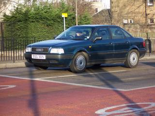
HIM parses the scene using a hierarchy of segmentations, as illustrated in Fig. 1. By incorporating multiple different segmentations, this representation addresses the problem of scale ambiguity in images. Instead of performing (approximate) inference on a large random field defined over the regions, inference is broken down into a sequence of predictions. As illustrated in Fig. 1, a predictor $f$ is associated with each level in the hierarchy that predicts the probability distribution of classes/objects contained within each region. These predictions are then used by the subsequent predictor in the next level (in addition to features derived from the image statistics) to make refined predictions on the finer regions; and the process iterates. By passing class distributions between predictors, contextual information is modeled even though the segmentation at any particular level may be incorrect. We note that while Fig. 1 illustrates a top-down sequence over the hierarchy, in practice, the authors iterate up and down the hierarchy which we also do in our comparison experiments.

4.3 Speedy Inference Machines

While HIM decomposes the structured prediction problem into an efficient sequence of predictions, it is not readily suited for an anytime prediction. First, the final predictions are generated when the procedure terminates at the leaf nodes in the hierarchy. Hence, interrupting the procedure before then would result in final predictions over coarse regions that may severely undersegment the scene. Second, the amount of computation time at each step of the procedure is invariant to the current performance. Because the structure of the sequence is predefined, the inference procedure will predict multiple times on a region as it traverses over the hierarchy, even though there may be no room for improvement. Third, the input to each predictor in the sequence is a fixed feature descriptor for the region. Because these input descriptors must be precomputed for all regions in the hierarchy before the inference process begins, there is a fixed initial computational cost. In the following, we describe how StructuredSpeedBoost addresses these three problems three problems for anytime scene understanding.

4.3.1 Interruptible Prediction

In order to address the first issue, we learn an additive predictor $f$ which predicts a per-pixel classification for the entire image at once. In contrast to HIM whose multiple predictors’ losses are measured over regions, we train a single predictor whose loss is measured over pixels. Concretely, given per-pixel ground truth distributions $p_{j}\in\mathbb{R}^{K}$, we wish to optimize per-pixel, cross-entropy risk for all pixels in the image

$$\mathcal{R}[f]=\mathbb{E}_{\mathcal{X}}\left[-\sum_{j}\sum_{k}p_{jk}\log q(f(x))_{jk}\right],$$ (18)

where

$$q(y)_{jk}=\frac{\exp(y_{jk})}{\sum_{k^{\prime}}\exp(y_{jk^{\prime}})},$$ (19)

i.e., the probability of the $k$’th class for the $j$’th pixel. Using (Eq. 12), the probability distribution associated with each pixel is then dependent on 1) the pixels to update, selected by $h_{\textrm{S}}$, and 2) the value of the predictor $h_{\textrm{P}}$ evaluated on those respective pixels. The definition of these functions are defined in the following subsections.

	Sky	Tree	Road	Grass	Water	Bldg.	Mtn.	Object	Class	Pixel
SIM	92.4	73.3	90.6	83.0	62.5	76.9	10.5	63.8	69.1	78.8
HIM [19]	92.9	77.5	89.9	83.6	70.9	83.2	17.2	69.3	73.1	82.1
[6]	95.7	78.7	88.1	89.7	68.7	79.9	44.6	62.3	76.0	81.4
[21]	-	-	-	-	-	-	-	-	-	78.1

	Bldg.	Tree	Sky	Car	Sign	Road	Ped.	Fence	Pole	Sdwlk.	Bike	Class	Pixel
SIM	76.8	79.2	94.1	71.8	30.2	95.2	34.6	25.7	14.0	66.3	15.0	54.8	81.5
HIM [19]	83.3	82.2	95.9	75.2	42.2	96.0	38.6	21.5	13.6	72.1	33.3	59.4	84.9
[5]	59	75	93	84	45	90	53	27	0	55	21	54.7	75.0
[17]†	81.5	76.6	96.2	78.7	40.2	93.9	43.0	47.6	14.3	81.5	33.9	62.5	83.8

Table 1: Recalls on the Stanford Background Dataset (top) and CamVid (bottom) where Class is the average per-class recall and Pixel is the per-pixel accuracy. ^†Uses additional training data not leveraged by other techniques.

4.3.2 Structure Selection and Prediction

In order to account for scale ambiguity and structure in the scene, we can similarly integrate multiple regions into our predictor. By using a hierarchical segmentation of the scene that produces many segments/regions, we can consider each resulting region or segment of pixels $S$ in the hierarchy as one possible set of outputs to update. Intuitively, there is no need to update regions of the image where the predictions are correct at the current inference step. Hence, we want to update the portion of the scene where the predictions are uncertain, i.e., have high entropy $H$. To achieve this, we use a selector function that selects regions that have high average per-pixel entropies in the current predictions,

$$h_{\textrm{S}}(x,\hat{y})=\left\{S\ \middle|\ \frac{1}{|S|}\sum_{j\in S}H(q(\hat{y})_{j})>\theta\right\},$$ (20)

for some fixed threshold $\theta$. In practice, the set of predictors $\mathcal{H}_{\textrm{S}}$ used at training time is created from a diverse set of thresholds $\theta$.

Additionally, we assume that the features $\psi_{j}$ used for each pixel in a given selected region are drawn from the entire region, so that if a given scale is selected features corresponding to that scale are used to update the selected pixels. For a given segment $S$, call this feature vector $\psi_{S}$.

Given the above selector function, we use (Eq. 14) to find the next best predictor function, as in Algorithm 1, optimizing

$$h_{\textrm{P}}^{*}=\underset{h_{\textrm{P}}}{\arg\min}\sum_{S\in h_{\textrm{S}}(x,\hat{y})}\sum_{j\in S}{\left\lVert{\nabla(x)_{j}-h_{\textrm{P}}(\psi_{S})}\right\rVert}^{2}.$$ (21)

Because all pixels in a given region use the same feature vector, this reduces to the weighted least squares problem:

$$h_{\textrm{P}}^{*}=\underset{h_{\textrm{P}}}{\arg\min}\sum_{S\in h_{\textrm{S}}(x,\hat{y})}|S|{\left\lVert{\nabla_{S}-h_{\textrm{P}}(\psi_{S})}\right\rVert}^{2}.$$ (22)

where $\nabla_{S}=\mathbb{E}_{j\in S}[\nabla(x)_{j}]=\mathbb{E}_{j\in S}[p_{j}-q(\hat{y})_{j}]$. In words, we find a vector-valued regressor $h_{\textrm{P}}$ with minimal weighted least squares error between the difference in ground truth and predicted per-pixel distributions, averaged over each selected region/segment, and weighted by the size of the selected region. This is an intuitive update that places large weight to updating large regions.

4.3.3 Dynamic Feature Computation

In the scene understanding problem, a significant computational cost during inference is often feature descriptor computation. To this end, we utilize the SpeedBoost cost model (Eq. 13) to automatically select the most computationally efficient features.

The features used in this application, drawn from previous work [11, 16] and detailed in the following section, are computed as follows. First, a set of base feature descriptors are computed from the input image data. In many applications it is useful to quantize these base feature descriptors and pool them together to form a set of derived features [2]. We follow the soft vector quantization approach in [2] to form a quantized code vector by computing distances to multiple cluster centers in a dictionary.

FH	SHAPE	TXT (B)	TXT (D)	LBP (B)	LBP (D)	I-SIFT (B)	I-SIFT (D)	C-SIFT (B)	C-SIFT (D)
167	2	29	66	64	265	33	165	93	443

Table 2: Average timings (ms) for computing all features for an image in the SBD. (B) is the time to compute the base per-pixel feature responses, and (D) is the time to compute the derived averaged-pooled region codes to all cluster centers.

This computation incurs a fixed cost for 1) each group of features with a common base feature, and 2) an additional, smaller fixed cost for each actual feature used. In order to account for these costs, we use an additive model similar to Xu et al. [29]. Formally, let $\phi\in\Phi$ be the set of features and $\gamma\in\Gamma$ be the set of feature groups, and $c_{\phi}$ and $c_{\gamma}$ be the cost for computing derived feature $\phi$ and the base feature for group $\gamma$, respectively. Let $\Phi(f)$ be the set of features used by predictor $f$ and $\Gamma(f)$ the set of its used groups. Given a current predictor $f_{t-1}$, its group and derived feature costs are then just the costs of any new group and derived features and have not previously been computed:

$$c_{\Gamma}(h_{\textrm{P}}) =\sum_{\gamma\in\Gamma(h_{\textrm{P}})\setminus\Gamma(f_{t-1})}c_{\gamma},$$ (23)

$$c_{\Phi}(h_{\textrm{P}}) =\sum_{\phi\in\Phi(h_{\textrm{P}})\setminus\Phi(f_{t-1})}c_{\phi}.$$ (24)

The total cost model in (Eq. 13) can then be derived using the sum of the feature costs and group costs as

$$c(h) =c(h_{\textrm{s}})+c(h_{\textrm{P}})$$ (25)

$$=\epsilon_{\textrm{S}}+\epsilon_{\textrm{P}}+c_{\Gamma}(h_{\textrm{P}})+c_{\Phi}(h_{\textrm{P}}),$$ (26)

where $\epsilon_{\textrm{S}}$ and $\epsilon_{\textrm{P}}$ are small fixed costs for evaluating a selection and prediction function, respectively.

In order to generate $h_{\textrm{P}}$ with a variety of costs, we use a modified regression tree that penalizes each split based on its potential cost, as in [29]. This approach augments the least-squares regression tree impurity function with a cost regularizer:

$$\mathbb{E}_{D}\left[w_{D}{\left\lVert{y_{D}-h_{\textrm{P}}(x_{D})}\right\rVert}^{2}\right]+\lambda\left(c_{\Gamma}(h_{\textrm{P}})+c_{\Phi}(h_{\textrm{P}})\right),$$ (27)

where $\lambda$ regularizes the cost. In addition to (Eq. 25), training regression trees with different values of $\lambda$, enables StructuredSpeedBoost to automatically select the most cost-efficient predictor.

5 Experimental Analysis

5.1 Setup

We evaluate performance metrics between SIM and HIM on the 1) Stanford Background Dataset (SBD) [10], which contains 8 classes, and 2) Cambridge Video Dataset (CamVid) [1], which contains 11 classes; we follow the same training/testing evaluation procedures as originally described in the respective papers. As shown in Table 1, we note that HIM achieves state-of-the-art performance and these datasets and analyze the computational tradeoffs when compared with SIM. Since both methods operate over a region hierarchy of the scene, we use the same segmentations, features, and regression trees (weak predictors) for a fair comparison.

5.1.1 Segmentations

We construct a 7-level segmentation hierarchy by recursively executing the graph-based segmentation algorithm (FH) [7] with parameters

$$\sigma =0.25,c=10^{2}\times[1,2,5,10,50,200,500],$$

$$k =[30,50,50,100,100,200,300].$$

These values were qualitatively chosen to generate regions at different resolutions.

5.1.2 Features

A region’s feature descriptor is composed of 5 feature groups ($\Gamma$): 1) region boundary shape/geometry/location (SHAPE) [11], 2) texture (TXT), 3) local binary patterns (LBP), 4) SIFT over intensity (I-SIFT), 5) SIFT separately over colors R, G, and B (C-SIFT). The last 4 are derived from per-pixel descriptors for which we use the publicly available implementation from [16].

Figure 2: Average pixel classification accuracy for SBD (top) and CamVid (bottom) datasets as a function of inference time.

Computations for segmentation and features are shown in Table 2; all times were computed on an Intel i7-2960XM processor. The SHAPE descriptor is computed solely from the segmentation boundaries and is efficient to compute. The remaining 4 feature group computations are broken down into the per-pixel descriptor (base) and the average-pooled vector quantized codes (derived), where each of the 4 groups are quantized separately with a dictionary size of 150 elements/centers using k-means. For a given pixel descriptor, $\upsilon$, its code assignment to cluster center, $\mu_{i}$, is derived from its squared $L_{2}$ distance $d_{i}(\upsilon)={\left\lVert{\upsilon-\mu_{i}}\right\rVert}_{2}^{2}$. Using the soft code assignment from [2], the code is defined as $\max(0,z_{i}(\upsilon))$, where

$$z_{i}(\upsilon) =\mathbb{E}_{j}[d_{j}(\upsilon)]-d_{i}(\upsilon)$$ (28)

$$=\mathbb{E}_{j}[\|\mu_{j}\|^{2}]-2{\left\langle{\mathbb{E}_{j}[\mu_{j}]},{\upsilon}\right\rangle}-(\|\mu_{i}\|^{2}-2{\left\langle{\mu_{i}},{\upsilon}\right\rangle}).$$ (29)

Note that the expectations are indepndent from the query descriptor $v$, hence the $i$’th code can be computed independently and enables selective computation for the region. The resulting quantized pixel codes are then averaged within each region. Thus, the costs to use these derived features are dependent if the pixel descriptor has already been computed or not. For example, when the weak learner first uses codes from the I-SIFT group, the cost incurred is the time to compute the I-SIFT pixel descriptor plus the time to compute distances to each specified center.

— Sky

— Tree

— Road

— Grass

— Water

— Building

— Mountain

— Object

— Building   — Tree   — Sky   — Car   — Sign   — Road   — Person   — Fence   — Pole   — Sidewalk   — Bicyclist

Figure 3: Sequence of images displaying the inferred labels and selected regions at iterations $t=\{1,5,15,50,100,225\}$ of the SIM algorithm for a sample image from the Stanford Background (top) and CamVid (bottom) datasets. The corresponding inference times for these iterations are $\{0.42s,0.44s,0.47s,0.79s,1.07s,1.63s\}$ (top) and $\{0.41s,0.42s,0.44s,0.52s,0.85s,1.42s\}$ (bottom).

— TXT

— I-SIFT

— C-SIFT

— LBP

Figure 4: The number of cluster centers selected within each feature group by SIM as a function of inference time.

5.2 Analysis

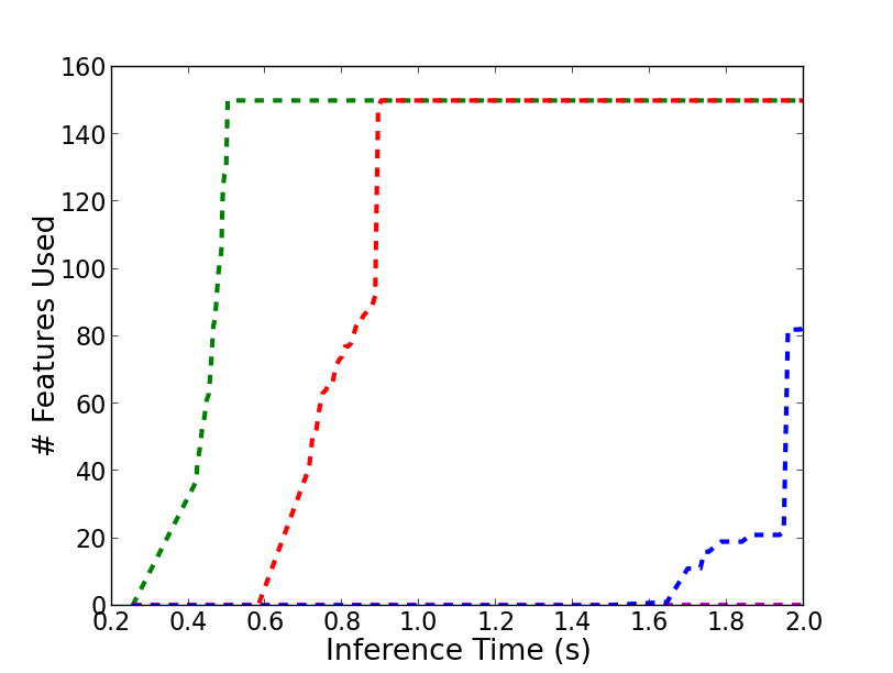
In Fig. 4 we show which cluster centers, from each of the four groups, are being selected by SIM as the inference time increases. We note that efficient SHAPE descriptor is chosen on the first iteration, followed by the next cheapest descriptors TXT and I-SIFT. Although LBP is cheaper than C-SIFT, the algorithm ignored LBP because it did not improve prediction wrt cost.

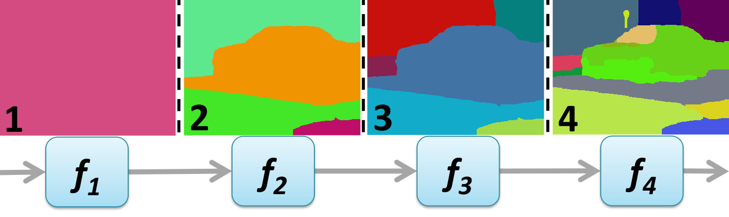
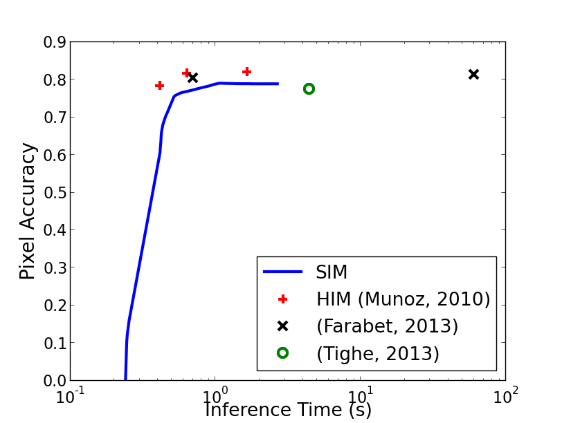
In Fig. 2, we compare the classification performance of SIM and several other algorithms with respect to inference time. We consider HIM as well as two variants which use a limited set of the 4 feature groups (only TXT and TXT & I-SIFT); these SIM and HIM models were executed on the same computer. We also compare to the reported performances of other techniques and stress that these timings are reported from different computing configurations. The single anytime predictor generated by our anytime structured prediction approach is competitive with all of the specially trained, standalone models without requiring any of the manual analysis necessary to create the different fixed models.

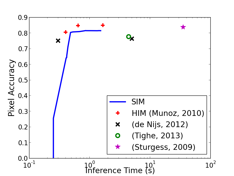
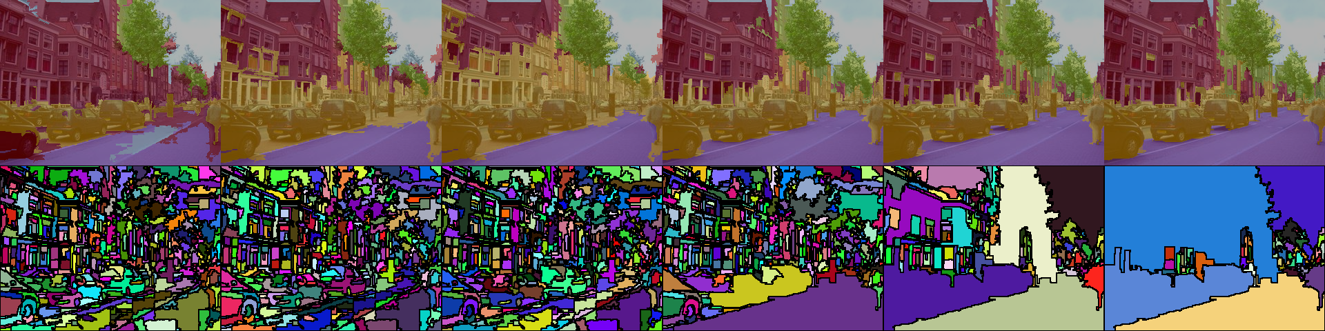
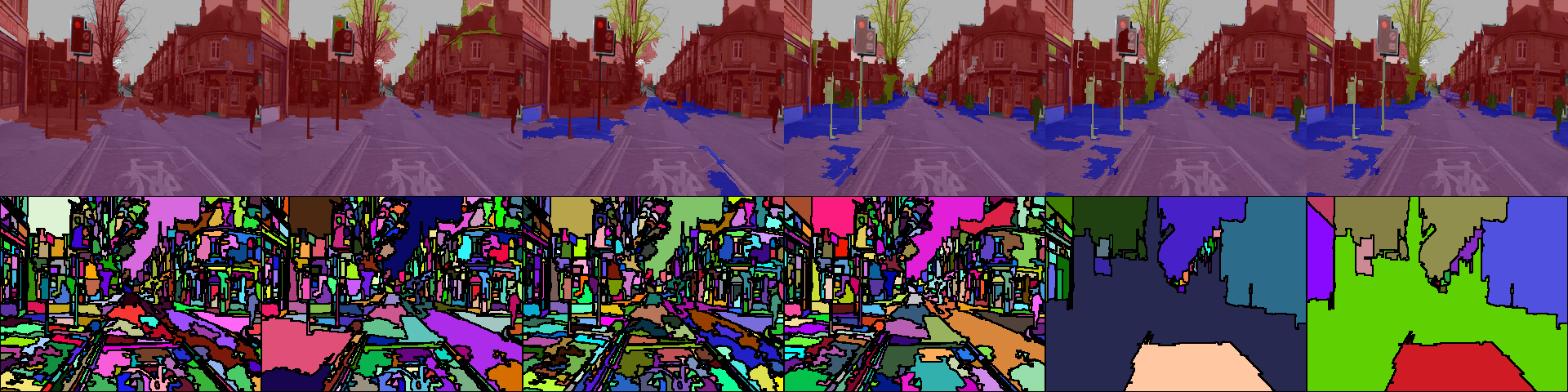
In Fig. 3, we show the progress of the SIM algorithm as it processes a scene from each of the datasets. Over time, we see the different structural nodes (regions) selected by the algorithm as well as improving classification.

6 Conclusion

We proposed a technique for structured prediction with anytime properties. Our approach is based under the boosting framework that automatically incorporates new learners to our predictor that best increases performance with respect to efficiency in terms of both feature and inference computation times. We demonstrated the efficacy of our approach on the challenging task of scene understanding in computer vision and achieved state-of-the-art performance classifications with improved efficiency over previous work.

References

- [1] Gabriel J. Brostow, Jamie Shotton, Julien Fauqueur, and Roberto Cipolla. Segmentation and recognition using structure from motion point clouds. In ECCV, 2008.
- [2] Adam Coates, Honglak Lee, and Andrew Y. Ng. An analysis of single-layer networks in unsupervised feature learning. In AISTATS, 2011.
- [3] William W. Cohen and Vitor Carvalho. Stacked sequential learning. In IJCAI, 2005.
- [4] Hal Daume III, John Langford, and Daniel Marcu. Search-based structured prediction. MLJ, 75(3), 2009.
- [5] Roderick de Nijs, Sebastian Ramos, Gemma Roig, Xavier Boix, Luc Van Gool, and Kolja Kuhnlenz. On-line semantic perception using uncertainty. In IROS, 2012.
- [6] Clement Farabet, Camille Couprie, Laurent Najman, and Yann LeCun. Learning hierarchical features for scene labeling. In T-PAMI, 2013.
- [7] Pedro F. Felzenszwalb and Daniel P. Huttenlocher. Efficient graph-based image segmentation. IJCV, 59(2), 2004.
- [8] J. H. Friedman. Greedy function approximation: A gradient boosting machine. Annals of Statistics, 29(5), 2001.
- [9] Tianshi Gao and Daphne Koller. Active classification based on value of classifier. In NIPS, 2011.
- [10] Stephen Gould, Richard Fulton, and Daphne Koller. Decomposing a scene into geometric and semantically consistent regions. In ICCV, 2009.
- [11] Stephen Gould, Jim Rodgers, David Cohen, Gal Elidan, and Daphne Koller. Multi-class segmentation with relative location prior. IJCV, 80(3), 2008.
- [12] Alexander Grubb and J. Andrew Bagnell. Speedboost: Anytime prediction with uniform near-optimality. In AISTATS, 2012.
- [13] Jiarong Jiang, Adam Teichert, Hal Daume III, and Jason Eisner. Learned prioritization for trading off accuracy and speed. In NIPS, 2012.
- [14] Sergey Karayev, Tobias Baumgartner, Mario Fritz, and Trevor Darrell. Timely object recognition. In NIPS, 2012.
- [15] Sanjiv Kumar and Martial Hebert. Discriminative random fields. IJCV, 68(2), 2006.
- [16] Lubor Ladicky. Global Structured Models towards Scene Understanding. PhD thesis, Oxford Brookes University, 2011.
- [17] Lubor Ladicky, Paul Sturgess, Karteek Alahari, Chris Russell, and Philip H.S. Torr. What, where & how many? combining object detectors and crfs. In ECCV, 2010.
- [18] L. Mason, J. Baxter, P. L. Bartlett, and M. Frean. Functional gradient techniques for combining hypotheses. In Advances in Large Margin Classifiers. MIT Press, 1999.
- [19] Daniel Munoz, J. Andrew Bagnell, and Martial Hebert. Stacked hierarchical labeling. In ECCV, 2010.
- [20] S. Ross, D. Munoz, M. Hebert, and J. A. Bagnell. Learning message-passing inference machines for structured prediction. In CVPR, 2011.
- [21] Richard Socher, Cliff Lin, Andrew Y. Ng, and Christopher D. Manning. Parsing natural scenes and natural language with recursive neural networks. In ICML, 2011.
- [22] Paul Sturgess, Karteek Alahari, Lubor Ladicky, and Philip H. S. Torr. Combining appearance and structure from motion features for road scene understanding. In BMVC, 2009.
- [23] Paul Sturgess, Lubor Ladicky, Nigel Crook, and Philip H. S. Torr. Scalable cascade inference for semantic image segmentation. In BMVC, 2012.
- [24] Joseph Tighe and Svetlana Lazebnik. Superparsing: Scalable nonparametric image parsing with superpixels. IJCV, 2013.
- [25] Zhuowen Tu and Xiang Bai. Auto-context and its application to high-level vision tasks and 3d brain image segmentation. T-PAMI, 32(10), 2010.
- [26] Paul A. Viola and Michael J. Jones. Robust real-time face detection. IJCV, 57(2), 2004.
- [27] David Weiss and Ben Taskar. Structured prediction cascades. In AISTATS, 2010.
- [28] David H. Wolpert. Stacked generalization. Neural Networks, 5(2), 1992.
- [29] Zhixiang Xu, Kilian Q. Weinberger, and Olivier Chapelle. The greedy miser: Learning under test-time budgets. In ICML, 2012.