Tunneling of Massive Dirac Fermions in Graphene
through Time-periodic Potential

Ahmed Jellal^a,b, Miloud Mekkaoui^b, El Bouâzzaoui Choubabi^b,c and Hocine Bahlouli^a,d

^aSaudi Center for Theoretical Physics, Dhahran, Saudi Arabia

^bTheoretical Physics Group, Faculty of Sciences, Chouaïb Doukkali University,

PO Box 20, 24000 El Jadida, Morocco

^cPhysics Department, Faculty Polydisciplinary, Sultan Moulay Slimane University,
23000 Beni Mellal, Morocco

^dPhysics Department, King Fahd University of Petroleum $\&$ Minerals,
Dhahran 31261, Saudi Arabia

The energy spectrum of a graphene sheet subject to a single barrier potential having a time periodic oscillating height and subject to a magnetic field is analyzed. The corresponding transmission is studied as function of the incident energy and potential parameters. Quantum interference within the oscillating barrier has an important effect on quasiparticles tunneling. In particular the time-periodic electrostatic potential generates additional sidebands at energies $\epsilon+l\hbar\omega$ ($l=0,\pm 1,\cdots$) in the transmission probability originating from the photon absorption or emission within the oscillating barrier. Due to numerical difficulties in truncating the resulting coupled channel equations we limited ourselves to low quantum channels, i.e. $l=0,\pm 1$.

PACS numbers: 73.63.-b; 73.23.-b; 72.80.Rj

Keywords: graphene, single barrier, Dirac equation, time dependent, transmission.

1 Introduction

Graphene [1] is a single layer of carbon atoms arranged into a planar honeycomb lattice. This system has attracted a considerable attention from both experimental and theoretical researchers since its experimental realization in 2004 [2]. This is because of its unique and outstanding mechanical, electronic, optical, thermal and chemical properties [3]. Most of these marvelous properties are due to the apparently relativistic-like nature of its carriers, electrons behave as massless Dirac fermions in graphene systems. In fact starting from the original tight-binding Hamiltonian describing graphene it has been shown theoretically that the low-energy excitations of graphene appear to be massless chiral Dirac fermions. Thus, in the continuum limit one can analyze the crystal properties using the formalism of quantum electrodynamics in (2+1)-dimensions. This similarity between condensed matter physics and quantum electrodynamics (QED) provides the opportunity to probe many physical aspects proper to high energy physics phenomena in condensed matter systems. Thus, in this regard, graphene can be considered as a test-bed laboratory for high energy relativistic quantum phenomena.

Quantum transport in periodically driven quantum systems is an important subject not only of academic value but also for device and optical applications. In particular quantum interference within an oscillating time-periodic electromagnetic field gives rise to additional sidebands at energies $\epsilon+l\hbar\omega$ $(l=0,\pm 1,\cdots)$ in the transmission probability originating from the fact that electrons exchange energy quanta $\hbar\omega$ carried by photons of the oscillating field, $\omega$ being the frequency of the oscillating field. The standard model in this context is that of a time-modulated scalar potential in a finite region of space. It was studied earlier by Dayem and Martin [4] who provided the experimental evidence of photon assisted tunneling in experiments on superconducting films under microwave fields. Later on Tien and Gordon [5] provided the first theoretical explanation of these experimental observations. Further theoretical studies were performed later by many research groups, in particular Buttiker investigated the barrier traversal time of particles interacting with a time-oscillating barrier [6]. Wagner [7] gave a detailed treatment on photon-assisted tunneling through a strongly driven double barrier tunneling diode and studied the transmission probability of electrons traversing a quantum well subject to a harmonic driving force [8] where transmission side-bands have been predicted. Grossmann [9], on the other hand, investigated the tunneling through a double-well perturbed by a monochromatic driving force which gave rise to unexpected modifications in the tunneling phenomenon.

In [10] the authors studied the chiral tunneling through a harmonically driven potential barrier in a graphene monolayer. Because the charge carriers in their system are massless they described the tunneling effect as the Klein tunneling with high anisotropy. For this, they determined the transmission probabilities for the central band and sidebands in terms of the incident angle of the electron beam. Subsequently, they investigated the transmission probabilities for varying width, amplitude and frequency of the oscillating barrier. They conclude that the perfect transmission for normal incidence, which has been reported for a static barrier, persists for the oscillating barrier that is a manifestation of Klein tunneling in a time-harmonic potential.

The growing experimental interest in studying optical properties of electron transport in graphene subject to strong laser fields [11] motivated the recent upsurge in theoretical study of the effect of time dependent periodic electromagnetic field on electron spectra. Recently it was shown that laser fields can affect the electron density of states and consequently the electron transport properties [12]. Electron transport in graphene generated by laser irradiation was shown to result in subharmonic resonant enhancement [13]. The analogy between spectra of Dirac fermions in laser fields and the energy spectrum in graphene superlattice formed by static one dimensional periodic potential was performed in [14]. In graphene systems resonant enhancement of both electron backscattering and currents across a scalar potential barrier of arbitrary space and time dependence was investigated in [15] and resonant sidebands in the transmission due to a time modulated potential region was studied recently in graphene [16]. The fact that an applied oscillating field can result in an effective mass or equivalently a dynamic gap was confirmed in recent studies [17]. Adiabatic quantum pumping of a graphene devise with two oscillating electric barriers was considered in [18]. A Josephson-like current was predicted for several time dependent scalar potential barriers placed upon a monolayer of graphene [19]. Stochastic resonance like phenomenon [20] was predicted for transport phenomena in disordered graphene nanojunctions [21]. Further study showed that noise-controlled effects can be induced due to the interplay between stochastic and relativistic dynamics of charge carriers in graphene [22].

In this work we generalize the results obtained in [10] in the presence of a magnetic field case. More precisely, we consider one monolayer graphene sheet lying in the $xy$-plane and subject to a scalar square potential barrier along the $x$-direction while the carriers are free in the $y$-direction. The barrier height oscillates sinusoidally around an average value $V_{0}$ with oscillation amplitude $V_{1}$ and frequency $\omega$. We calculate the transmission probability for the central band and close by sidebands as a function of the potential parameters and incident angle of the particles. The limitation to close by sidebands is due to numerical difficulties in truncating the resulting coupled channel equations which forced us to limit ourselves to low quantum channels.

The manuscript is organized as follows. In section 2, we present the theoretical model describing the graphene sheet in the presence of an external magnetic field and oscillating barrier potential. In section 3, we explicitly determine the eigenvalues and corresponding eigenspinors for each regions composing ours system. We study the energy spectrum by investigating different properties to underline its behavior with respect to changes of physical parameters in section 4. The transmission through oscillating barrier will be analyzed in section 5 followed by a discussion of the numerical results in section 6. To complete our study, we deal with the total transmission probability in section 7. Our conclusions are given in the final section.

2 Theoretical model

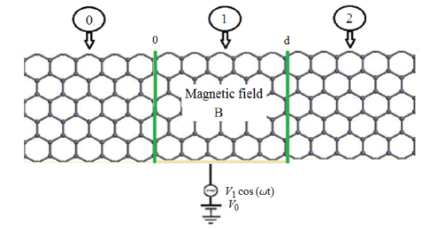
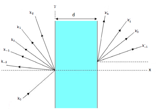
We study the tunneling effect of a system of Dirac fermions living in two-dimensions. This system is a flat sheet of graphene subject to a square potential barrier along the $x$-direction while particles are free in the $y$-direction. The width of the barrier is $d$, its height is oscillating sinusoidally around $V_{0}$ with amplitude $V_{1}$ and frequency $\omega$. The intermediate zone is subject to a magnetic field $\textbf{B}=B(x,y)\textbf{e}_{z}$ perpendicular to the graphene sheet. Electrons with energy $\epsilon={E}/{v_{F}}$ are incident from one side of the barrier with an angle $\phi_{0}$ with respect to the $x$-direction and leaves the barrier with energy $\epsilon+l\hbar\omega$ $(l=0,\pm 1,\cdots)$, which $l$ are the modes generated by oscillations and making angles $\pi-\phi_{l}$ after reflection and $\theta_{l}$ after transmission. The corresponding Hamiltonian can be split into two parts

$$H=H_{I}+H_{II}$$ (1)

such that the first one is

$$H_{I}=v_{F}{\boldsymbol{\sigma}}\cdot\left(-i\hbar{\boldsymbol{\nabla}}+\frac{e}{c}\textbf{A}(x,y)\right)+V(x){\mathbb{I}}_{2}$$ (2)

and the second one describes the harmonic time dependence of the barrier height

$$H_{II}=V_{j}\cos(\omega t)$$ (3)

where $\upsilon_{F}$ is the Fermi velocity, ${\boldsymbol{\sigma}}=(\sigma_{x},\sigma_{y})$ are the Pauli matrices and ${\mathbb{I}}_{2}$ is the $2\times 2$ unit matrix. $V$ and $V_{j}$ are the static square potential barrier and the amplitude of the oscillating potential, respectively. Both $V$ and $V_{j}$ are constants for $0\leq x\leq d$ with $d$ positive and are zero elsewhere, which can be summarized as

$$V(x)=\left\{\begin{array}[]{ll}V_{0},&\qquad\hbox{$0\leq x\leq d$}\\ 0,&\qquad\hbox{otherwise}\\ \end{array}\right.,\qquad V_{j}=\left\{\begin{array}[]{ll}V_{1},&\qquad\hbox{$0\leq x\leq d$}\\ 0,&\qquad\hbox{otherwise}\\ \end{array}\right.$$ (4)

and the script $j={\sf 0},{\sf 1},{\sf 2}$ denotes each scattering region. For a magnetic barrier, the relevant physics is described by a magnetic field translationally invariant along the $y$-direction, $B(x,y)=B(x)$. Choosing the Landau gauge we impose the vector potential ${\boldsymbol{A}}=(0,A_{y}(x))^{T}$ with $\partial_{x}A_{y}(x)=B(x)$, the transverse momentum $p_{y}$ is thus conserved. The magnetic field $\textbf{B}=B_{0}\textbf{e}_{z}$ (with constant $B_{0}$) within the strip $0\leq x\leq d$ but $B=0$ elsewhere, such as

$$B(x,y)=B_{0}\Theta(dx-x^{2})$$ (5)

with the Heaviside step function $\Theta$

$$\Theta(x)=\left\{\begin{array}[]{ll}1,&\qquad\hbox{$x>0$}\\ 0,&\qquad\hbox{otherwise.}\\ \end{array}\right.$$ (6)

Figure 1: (Color online) Schematic of an oscillating potential in a magnetic field of the monolayer graphene.

The continuity of the corresponding potential vector takes the following expression

$$\qquad A_{y}(x)=\left\{\begin{array}[]{ll}0,&\qquad\hbox{$x<0$}\\ B_{0}x,&\qquad\hbox{$0\leq x\leq d$}\\ B_{0}d,&\qquad\hbox{$x>d$}.\\ \end{array}\right.$$ (7)

Our system can be presented in Figure 1 to show clearly the oscillating potential in a magnetic field of the monolayer. On the light of this, we present in Figure 2 how the electrons can be scattered by our barrier potential. This will help to analyze the tunneling effect and calculate different physical quantities.

Figure 2: (Color online) Geometry of electron diffraction.

3 Energy spectrum

To explicitly determine the solutions of the energy spectrum of our theoretical model, we separately handle each part of the Hamiltonian (1). Thus, let us start from the time-dependent Dirac equation in the absence of oscillating potential for the spinor $\psi(x,y)=(\psi_{+},\psi_{-})^{T}$ at energy $E$. This is

$$H_{I}\psi(x,y,t)=E\psi(x,y,t)$$ (8)

where $\psi(x,y,t)=\psi(x,y)e^{-iEt/\hbar}$. In matrix form, we have

$$\left(\begin{array}[]{cc}0&-i\partial_{x}-\partial_{y}-\frac{ie}{\hbar c}A(x)\\ -i\partial_{x}+\partial_{y}+\frac{ie}{\hbar c}A(x)&0\\ \end{array}\right)\left(\begin{array}[]{c}\psi_{+}\\ \psi_{-}\\ \end{array}\right)=\frac{E}{\hbar\upsilon_{F}}\left(\begin{array}[]{c}\psi_{+}\\ \psi_{-}\\ \end{array}\right).$$ (9)

Since the transverse momentum $p_{y}$ is conserved, we can write the wave function in separable form $\psi_{\pm}(x,y)=\varphi_{\pm}(x)e^{ik_{y}y}$. Thus after rescaling energy $\epsilon=E/v_{F}$ and using the unit system with $(\hbar=c=e=1)$, we obtain the two linear differential equations

$$\left(-i\partial_{x}-ik_{y}-iA(x)\right)\varphi_{-}=\epsilon\varphi_{+}$$ (10)

$$\left(-i\partial_{x}+ik_{y}+iA(x)\right)\varphi_{+}=\epsilon\varphi_{-}.$$ (11)

This can be combined to describe the solution of (9) and then consider the incoming electrons to be in plane wave states $\psi_{inc}(x,y,t)$ at energy $\epsilon$ as

$$\psi_{inc}(x,y,t)=\left(\begin{array}[]{c}1\\ \alpha_{0}\end{array}\right)e^{ik_{0}x}e^{ik_{y}y}e^{-iv_{F}\epsilon t}$$ (12)

where $\alpha_{0}$ is given by

$$\alpha_{0}=s_{0}\frac{k_{0}+ik_{y}}{\sqrt{k_{0}^{2}+k_{y}^{2}}}=s_{0}e^{\textbf{\emph{i}}\phi_{0}}$$ (13)

with $s_{0}=\mbox{sgn}(\epsilon)$, $\phi_{0}$ is the angle that the incident electrons make with the $x$-direction, $k_{0}$ and $k_{y}$ are the $x$ and $y$-components of the electron wave vector, respectively. After rescaling the potential $v_{j}=V_{j}/v_{F}$ and frequency $\varpi=\omega/v_{F}$, we show that the transmitted and reflected waves have components at all energies $\epsilon+l\varpi$ $(l=0,\pm 1,\cdots)$. Indeed the wave functions $\psi_{r}(x,y,t)$ for reflected electrons are

$$\psi_{r}(x,y,t)=\sum^{+\infty}_{m,l=-\infty}r_{l}\left(\begin{array}[]{c}1\\ -\frac{1}{\alpha_{l}}\end{array}\right)e^{-ik_{l}x+ik_{y}y}J_{m-l}\left(\frac{v_{j}}{\varpi}\right)\ e^{-iv_{F}(\epsilon+m\varpi)t}$$ (14)

and the corresponding energy reads as

$$\epsilon+l\varpi=s_{l}\sqrt{k^{2}_{l}+k^{2}_{y}}$$ (15)

where $r_{l}$ is the reflection amplitude and $J_{m}\left(\frac{v_{1}}{\varpi}\right)$ is the Bessel function of the first kind. Note that, for the modulation amplitude $v_{j}=0$ we have $J_{m-l}\left(0\right)=\delta_{ml}$. We will return to this point once we talk about the solution in different regions composing the graphene sheet. The parameter $\alpha_{l}$ is the complex number

$$\alpha_{l}=s_{l}\frac{k_{l}+ik_{y}}{\sqrt{k^{2}_{l}+k_{y}^{2}}}=s_{l}\ e^{\textbf{\emph{i}}\phi_{l}}$$ (16)

where $\phi_{l}=\tan^{-1}(k_{y}/k_{l})$, $s_{l}=\mbox{sgn}(\epsilon+l\varpi)$, the sign again refers to conduction and valence bands of region. The wave vector $k_{l}$ for mode $l$ can be obtained from (15)

$$k_{l}=s_{l}\sqrt{\left(\epsilon+l\varpi\right)^{2}-k^{2}_{y}}.$$ (17)

While, the wave functions $\psi_{t}(x,y,t)$ for transmitted electrons read as

$$\psi_{t}(x,y,t)=\sum^{+\infty}_{m,l=-\infty}t_{l}\left(\begin{array}[]{c}1\\ \beta_{l}\end{array}\right)e^{ik^{{}^{\prime}}_{l}x+ik_{y}y}J_{m-l}\left(\frac{v_{j}}{\varpi}\right)e^{-iv_{F}(\epsilon+m\varpi)t}$$ (18)

and the eigenvalues are

$$\epsilon+l\varpi=s_{l}\sqrt{k^{{}^{\prime}2}_{l}+\left(k_{y}+\frac{d}{l^{2}_{B}}\right)^{2}}$$ (19)

where $l_{B}=\sqrt{1/B_{0}}$ is the magnetic length , $t_{l}$ is the transmission amplitude and different parameters are given by

$$\beta_{l}=s_{l}\frac{k^{{}^{\prime}}_{l}+i\left(k_{y}+\frac{d}{l^{2}_{B}}\right)}{\sqrt{k^{{}^{\prime}2}_{l}+\left(k_{y}+\frac{d}{l^{2}_{B}}\right)^{2}}}=s_{l}\ e^{\textbf{\emph{i}}\theta_{l}}$$ (20)

$$k^{{}^{\prime}}_{l}=s_{l}\sqrt{\left(\epsilon+l\varpi\right)^{2}-\left(k_{y}+\frac{d}{l^{2}_{B}}\right)^{2}}$$ (21)

$$\theta_{l}=\tan^{-1}\left[\left(k_{y}+\frac{d}{l^{2}_{B}}\right)/k^{{}^{\prime}}_{l}\right].$$ (22)

At this level we summarize our solutions by writing the scattering states in different regions. Recall that, in regions ${\sf 0}$ and ${\sf 2}$ the potential height is $v_{j}=0$, then we proceed by replacing $J_{m-l}$ by $\delta_{ml}$. Consequently, in region ${\sf 0}$, i.e. $x<0$, we have

$$\psi_{\sf 0}(x,y,t)=e^{ik_{y}y}\sum^{+\infty}_{m,l=-\infty}\left[\delta_{l0}\left(\begin{array}[]{c}1\\ \alpha_{l}\end{array}\right)e^{ik_{l}x}+r_{l}\left(\begin{array}[]{c}1\\ -\frac{1}{\alpha_{l}}\end{array}\right)e^{-ik_{l}x}\right]\delta_{ml}\ e^{-iv_{F}(\epsilon+m\varpi)t}$$ (23)

and region ${\sf 2}$ $(x>d)$

$$\psi_{\sf 2}(x,y,t)=e^{ik_{y}y}\sum^{+\infty}_{m,l=-\infty}\left[t_{l}\left(\begin{array}[]{c}1\\ \beta_{l}\end{array}\right)e^{ik^{{}^{\prime}}_{l}x}+b_{l}\left(\begin{array}[]{c}1\\ -\frac{1}{\beta_{l}}\end{array}\right)e^{-ik^{{}^{\prime}}_{l}x}\right]\delta_{ml}\ e^{-iv_{F}(\epsilon+m\varpi)t}$$ (24)

where $\{b_{l}\}$ is a set of the null vectors.

In the barrier region ${\sf 1}$ $(0\leq x\leq d)$, where $H_{II}$ is non-zero, the eigenfunctions $\psi_{\sf 1}(x,y,t)$ of the total Hamiltonian $H$ can be expressed in terms of the eigenfunctions $\psi_{1}(x,y)$ at energy $\epsilon$ of $H_{I}$. These are given by

$${\psi_{\sf 1}(x,y,t)=\psi_{1}(x,y)\sum^{+\infty}_{m=-\infty}J_{m}\left(\alpha\right)\ e^{-iv_{F}(\epsilon+\varpi m)t}}$$ (25)

where we have set $\alpha={v_{1}}/{\varpi}$. To include all modes, a linear combination of wave functions at energies $\epsilon_{l}=\epsilon+l\varpi$ $(l=0,\pm 1,\cdots)$ has to be taken. Hence, one has to write (25) as

$$\psi_{\sf 1}(x,y,t)=\sum^{+\infty}_{l=-\infty}\psi_{l}(x,y)\sum^{+\infty}_{m=-\infty}J_{m}\left(\alpha\right)\ e^{-iv_{F}(\epsilon+\varpi(l+m))t}$$ (26)

where eigenspinors $\psi_{l}(x,y)$ are solution of the following equation

$$\left[{\boldsymbol{\sigma}}\cdot{\boldsymbol{\pi}_{l}}+\frac{1}{v_{F}}V{\mathbb{I}}_{2}\right]\psi_{l}(x,y)=\epsilon_{l}\psi_{l}(x,y)$$ (27)

with $\pi_{lx}=p_{lx}$ and $\pi_{y}=p_{y}+A_{y}$. The $y$-component of the momentum is a constant of motion and the spinor wave function can be written as $\psi_{l}(x,y)=\varphi_{l}(x)e^{ik_{y}y}.$ We solve the eigenvalue equation for a given spinor $\varphi_{l}=(\varphi_{l,1},\varphi_{l,2})^{T}$

$$\left(\begin{array}[]{cc}V/v_{F}&-i\left(\partial_{lx}+k_{y}+\frac{x}{l_{B}^{2}}\right)\\ i\left(-\partial_{lx}+k_{y}+\frac{x}{l_{B}^{2}}\right)&V/v_{F}\\ \end{array}\right)\left(\begin{array}[]{c}\varphi_{l,1}\\ \varphi_{l,2}\\ \end{array}\right)=(\epsilon+l\varpi)\left(\begin{array}[]{c}\varphi_{l,1}\\ \varphi_{l,2}\\ \end{array}\right).$$ (28)

Defining the usual bosonic operators

$$a_{l}=\frac{l_{B}}{\sqrt{2}}\left(\partial_{lx}+k_{y}+\frac{x}{l_{B}^{2}}\right),\qquad a_{l}^{\dagger}=\frac{l_{B}}{\sqrt{2}}\left(-\partial_{lx}+k_{y}+\frac{x}{l_{B}^{2}}\right)$$ (29)

which satisfy the commutation relation $[a_{l},a_{k}^{\dagger}]=\delta_{lk}$. Rescaling our potential $v=V_{0}/v_{F}$, in terms of $a_{l}$ and $a_{l}^{\dagger}$ (28) reads as

$$\left(\begin{array}[]{cc}v&-i\frac{\sqrt{2}}{l_{B}}a_{l}\\ i\frac{\sqrt{2}}{l_{B}}a_{l}^{\dagger}&v\\ \end{array}\right)\left(\begin{array}[]{c}\varphi_{l,1}\\ \varphi_{l,2}\\ \end{array}\right)=(\epsilon+l\varpi)\left(\begin{array}[]{c}\varphi_{l,1}\\ \varphi_{l,2}\\ \end{array}\right)$$ (30)

which gives two relations between spinor components

$$-i\frac{\sqrt{2}}{l_{B}}a_{l}\varphi_{l,2}=(\epsilon+l\varpi-v)\varphi_{l,1}$$ (31)

$$i\frac{\sqrt{2}}{l_{B}}a_{l}^{\dagger}\varphi_{l,1}=(\epsilon+l\varpi-v)\varphi_{l,2}.$$ (32)

Now injecting (32) in (31), we obtain a differential equation of second order for $\varphi_{l,1}$

$$(\epsilon+l\varpi-v)^{2}\varphi_{l,1}=\frac{2}{l_{B}^{2}}a_{l}a_{l}^{\dagger}\varphi_{l,1}.$$ (33)

It is clear that $\varphi_{l,1}$ is an eigenstate of the number operator ${N_{l}}=a_{l}^{\dagger}a_{l}$ and therefore we identify $\varphi_{l,1}$ with the eigenstates of the harmonic oscillator

$$\varphi_{l,1}\sim\mid n_{l}-1\rangle$$ (34)

and the corresponding eigenvalues are given by

$$\epsilon_{l}=\epsilon+l\varpi=v\pm\frac{1}{l_{B}}\sqrt{2n_{l}}.$$ (35)

The second spinor component can be obtained from (32) to end up with

$$\varphi_{l,2}=\frac{i\sqrt{2n_{l}}}{\epsilon l_{B}+l\varpi l_{B}-vl_{B}}\mid n_{l}\rangle\varphi_{l,2}=\pm i\mid n_{l}\rangle$$ (36)

Thus, combining all to get the eigenspinors

$$\varphi_{l}^{\pm}=\left(\begin{array}[]{c}\mid n_{l}-1\rangle\\ \pm i\mid n_{l}\rangle\\ \end{array}\right)$$ (37)

where the wave functions $\varphi_{n_{l}}(x)=\langle x\mid n_{l}\rangle$ can be written in terms of the parabolic cylinder functions $D_{n_{l}}(Q)$ as

$$\varphi_{n_{l}}(x)=c_{n_{l}}D_{n_{l}}(Q),\qquad D_{n_{l}}(Q)=2^{-\frac{n_{l}}{2}}e^{-\frac{Q^{2}}{4}}H_{n_{l}}\left(\frac{Q}{\sqrt{2}}\right)$$ (38)

and and $H_{n_{l}}$ are the Hermite functions, $Q=\sqrt{2}\frac{x+x_{0}}{l_{B}}$ and $c_{n_{l}}=1/\sqrt{n_{l}!l_{B}^{2}\pi}$ which satisfy the recurrence relation $c_{n_{l}}=\frac{1}{\sqrt{n_{l}}}c_{n_{l}-1}.$ Finally, the solution in region ${\sf II}$ can be expressed as

$$\psi_{\sf 1}(x,y,t)=e^{ik_{y}y}\sum^{+\infty}_{m,l=-\infty}\sum_{\pm}c^{\pm}_{l}\left(\begin{array}[]{c}D_{1/\left(\Lambda_{l}\right)^{2}-1}\left[\pm\sqrt{2}\left(\frac{x}{l_{B}}+k_{y}l_{B}\right)\right]\\ \pm i\Lambda_{l}D_{1/\left(\Lambda_{l}\right)^{2}}\left[\pm\sqrt{2}\left(\frac{x}{l_{B}}+k_{y}l_{B}\right)\right]\\ \end{array}\right)J_{m-l}\left(\alpha\right)\ e^{-iv_{F}(\epsilon+m\varpi)t}$$ (41)

where we have set

$$\Lambda_{l}=\frac{\sqrt{2}}{l_{B}|\epsilon+l\varpi-v|}.$$ (42)

Having obtained all solutions of the energy spectrum, we will see how they can be used to deal with different issues. Specifically, the determination of transmission and reflection in terms of the different physical parameters of our system.

4 Spectrum properties

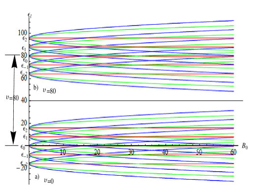
At this level let us study our eigenvalues to underline their basic features. From (35), we obtain the energy modulation due the oscillating potential as shown in Figure 3:

Figure 3: (Color online) Schematic oscillating barrier.

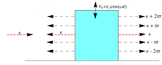
Figure 3 gives an idea how the energy spectrum looks like. It is clearly seen that absorbing energy quantum $\varpi$ produces interlevel transitions. Because of the Pauli principle an electron with energy $\epsilon$ can absorb an energy quantum $\varpi$ if only the state with energy $\epsilon+\varpi$ is empty. After absorbing the state with energy $\epsilon$ becomes empty, then one can write

$$\epsilon=v-l\varpi\pm\frac{1}{l_{B}}\sqrt{2n_{l}}$$ (43)

and from (35) we can each time fix $l$ to end up with the set of energies

$$\epsilon_{0}=\epsilon=v\pm\frac{1}{l_{B}}\sqrt{2n_{0}},\qquad\epsilon_{1}=\epsilon+\varpi=v\pm\frac{1}{l_{B}}\sqrt{2n_{1}},\qquad\epsilon_{2}=\epsilon+2\varpi=v\pm\frac{1}{l_{B}}\sqrt{2n_{2}}\ \cdots.$$ (44)

Note that, the energy conservation imposes the condition

$$\epsilon=v\pm\frac{1}{l_{B}}\sqrt{2n_{0}}=-\varpi+v\pm\frac{1}{l_{B}}\sqrt{2n_{1}}=-2\varpi+v\pm\frac{1}{l_{B}}\sqrt{2n_{2}}=\cdots=-l\varpi+v\pm\frac{1}{l_{B}}\sqrt{2n_{l}}$$ (45)

which implies that the energy for any integer value $l$ can be written as

$$\epsilon_{l}=v+l\varpi\pm\frac{1}{l_{B}}\sqrt{2n_{0}}.$$ (46)

It is clearly seen that the difference of energy is $\epsilon_{l+1}-\epsilon_{l}=\varpi$, which independent of the quantum numebr $n_{0}$. Combining all to present the energy in terms of the external magnetic field in Figure 4. One can notice that for $n_{0}=0$, we have just modulation of the energy with different number quanta $l\varpi$ with $l=0,\pm 1,\cdots$. However for $n_{0}=1,2$ the energy behavior is completely changed and for each $l$ value the energy is split into two values, which can be seen like a left of degeneracy of levels.

Figure 4: (Color online) Graphs depicting the energy $\epsilon_{l}$ as a function of magnetic field $B_{0}$, $\varpi=8$, potential $v=\{0,80\}$, $n_{0}=0$ (red), $n_{0}=1$ (green) and $n_{0}=2$ (blue).

5 Transmission through oscillating barrier

Note that for our system, as Dirac electrons pass through a region subjected to time-harmonic potentials, transitions from the central band to sidebands (channels) at energies $\epsilon+l\varpi$ $(l=0,\pm 1,\cdots)$ occur as electrons ex-change energy quanta with the oscillating field. Then to handle the propagation of waves, we need the transmission and reflection amplitudes, which can be determined by matching different wave functions at interfaces $0$ and $d$ to write

$$\psi_{\sf 0}(0,y,t)=\psi_{\sf 1}(0,y,t)$$ (47)

$$\psi_{\sf 1}(d,y,t)=\psi_{\sf 2}(d,y,t).$$ (48)

For simplify of writing, we use the shorthand notation

$$\eta_{1,l}^{\pm}=D_{1/\left(\Lambda_{l}\right)^{2}-1}\left(\pm\sqrt{2}k_{y}l_{B}\right)$$ (49)

$$\xi_{1,l}^{\pm}=D_{1/\left(\Lambda_{l}\right)^{2}}\left(\pm\sqrt{2}k_{y}l_{B}\right)$$ (50)

$$\eta_{2,l}^{\pm}=D_{1/\left(\Lambda_{l}\right)^{2}-1}\left[\pm\sqrt{2}\left(\frac{d}{l_{B}}+k_{y}l_{B}\right)\right]$$ (51)

$$\xi_{2,l}^{\pm}=D_{1/\left(\Lambda_{l}\right)^{2}}\left[\pm\sqrt{2}\left(\frac{d}{l_{B}}+k_{y}l_{B}\right)\right].$$ (52)

To derive different physical quantities, one can explicitly write (47-48) by making use the fact that the basis $\{e^{imv_{F}\varpi t}\}$ is orthogonal. Thus at interface $x=0$, one finds

$$\delta_{m0}+r_{m}=\sum^{+\infty}_{l=-\infty}\left(c^{+}_{l}\eta_{1,l}^{+}+c^{-}_{l}\eta_{1,l}^{-}\right)J_{m-l}\left(\alpha\right)$$ (53)

$$\delta_{m0}\alpha_{m}-r_{m}\frac{1}{\alpha_{m}}=\sum^{+\infty}_{l=-\infty}\left(c^{+}_{l}i\Lambda_{l}\xi_{1,l}^{+}-c^{-}_{l}i\Lambda_{l}\xi_{1,l}^{-}\right)J_{m-l}\left(\alpha\right)$$ (54)

at $x=d$ we have

$$t_{m}e^{ik^{{}^{\prime}}_{m}d}+b_{m}e^{-ik^{{}^{\prime}}_{m}d}=\sum^{+\infty}_{l=-\infty}\left(c^{+}_{l}\eta_{2,l}^{+}+c^{-}_{l}\eta_{2,l}^{-}\right)J_{m-l}\left(\alpha\right)$$ (55)

$$t_{m}\beta_{m}e^{ik^{{}^{\prime}}_{m}d}-b_{m}\frac{1}{\beta_{m}}e^{-ik^{{}^{\prime}}_{m}d}=\sum^{+\infty}_{l=-\infty}\left(c^{+}_{l}i\Lambda_{l}\xi_{2,l}^{+}-c^{-}_{l}i\Lambda_{l}\xi_{2,l}^{-}\right)J_{m-l}\left(\alpha\right).$$ (56)

It is convenient to write (53-56) in matrix form, such as

$$\left(\begin{array}[]{c}\Xi_{0}\\ \Xi_{0}^{{}^{\prime}}\\ \end{array}\right)=\left(\begin{array}[]{cc}{\mathbb{M}11}&{\mathbb{M}12}\\ {\mathbb{M}21}&{\mathbb{M}22}\\ \end{array}\right)\left(\begin{array}[]{c}\Xi_{2}\\ \Xi_{2}^{{}^{\prime}}\\ \end{array}\right)={\mathbb{M}}\left(\begin{array}[]{c}\Xi_{2}\\ \Xi_{2}^{{}^{\prime}}\\ \end{array}\right)$$ (65)

where the total transfer matrix ${\mathbb{M}}={\mathbb{M}(0,1)}\cdot{\mathbb{M}(1,2)}$ and ${\mathbb{M}(j,j+1)}$ are transfer matrices that couple the wave function in the $j$-th region to the wave function in the $(j+1)$-th region. These are given by

$${\mathbb{M}(0,1)}=\left(\begin{array}[]{cc}{\mathbb{I}}&{\mathbb{I}}\\ {\mathbb{N}_{1}^{+}}&{\mathbb{N}_{1}^{-}}\\ \end{array}\right)^{-1}\left(\begin{array}[]{cc}{\mathbb{C}_{1}^{+}}&{\mathbb{C}_{1}^{-}}\\ {\mathbb{G}_{1}^{+}}&{\mathbb{G}_{1}^{-}}\\ \end{array}\right)$$ (70)

$${\mathbb{M}(1,2)}=\left(\begin{array}[]{cc}{\mathbb{C}_{2}^{+}}&{\mathbb{C}_{2}^{-}}\\ {\mathbb{G}_{2}^{+}}&{\mathbb{G}_{2}^{-}}\\ \end{array}\right)^{-1}\left(\begin{array}[]{cc}{\mathbb{I}}&{\mathbb{I}}\\ {\mathbb{N}_{2}^{+}}&{\mathbb{N}_{2}^{-}}\\ \end{array}\right)\left(\begin{array}[]{cc}{\mathbb{K}^{+}}&{\mathbb{O}}\\ {\mathbb{O}}&{\mathbb{K}^{-}}\\ \end{array}\right)$$ (77)

where we have set the quantities

$$\left({\mathbb{N}_{1}^{\pm}}\right)_{m,l}=\pm\left(\alpha_{m}\right)^{\pm 1}\delta_{ml}$$ (78)

$$\left({\mathbb{C}_{\tau}^{\pm}}\right)_{m,l}=\eta_{\tau,l}^{\pm}J_{m-l}\left(\alpha\right)$$ (79)

$$\left({\mathbb{G}_{\tau}^{\pm}}\right)_{m,l}=\pm i\Lambda_{l}\xi_{\tau,l}^{\pm}J_{m-l}\left(\alpha\right)$$ (80)

$$\left({\mathbb{K}^{\pm}}\right)_{m,l}=\pm e^{\pm idk_{m}^{{}^{\prime}}}\delta_{ml}$$ (81)

$$\left({\mathbb{N}_{2}^{\pm}}\right)_{m,l}=\pm\left(\beta_{m}\right)^{\pm 1}\delta_{ml}$$ (82)

with the null matrix is denoted by ${\mathbb{O}}$ and ${\mathbb{I}}$ is the unit matrix. We assume an electron propagating from left to right with energy $\epsilon$ then $\tau=(1,2)$, $\Xi_{0}$ and the null vector $\Xi_{2}^{{}^{\prime}}$ read as

$$\Xi_{0}=\{\delta_{0l}\},\qquad\Xi_{2}^{{}^{\prime}}=\{b_{m}\}$$ (83)

whereas the vectors of transmitting and reflecting waves are given by

$$\Xi_{2}=\{t_{l}\},\qquad\Xi_{0}^{{}^{\prime}}=\{r_{l}\}.$$ (84)

From the above considerations, one can easily obtain the relation

$$\Xi_{2}=\left({\mathbb{M}11}\right)^{-1}\cdot\Xi_{0}.$$ (85)

The minimum number $N$ of sidebands that needs to be considered is determined by the strength of the oscillation, $N>\alpha$, and the infinite series for $T$ can be truncated to consider a finite number of terms starting from $-N$ up to $N$. Then (85) reduces

$$\left(\begin{array}[]{cc}t_{-N}\\ .\\ .\\ t_{-1}\\ t_{0}\\ t_{1}\\ .\\ .\\ t_{N}\\ \end{array}\right)=\left({\mathbb{M}11}\right)^{-1}\left(\begin{array}[]{cc}0\\ 0\\ 0\\ 0\\ 1\\ 0\\ 0\\ 0\\ 0\\ \end{array}\right)$$ (104)

where ${\mathbb{(}M11)^{-1}}$ becomes now a matrix of order $[2N+1,2N+1]$. This allows to end up with transmission amplitudes

$$t_{-N+k}=M^{\prime}\left[k+1,N+1\right]$$ (105)

with $k=0,1,\cdots,2N$ and $M^{\prime}$ is a matrix element of ${\mathbb{(}M11)^{-1}}$. Furthermore, analytical results are obtained if we consider small values of $\alpha={v_{1}}/{\varpi}$ and include only the first two sidebands at energies $\epsilon\pm\varpi$ along with the central band at energy $\epsilon$.

To explicitly determine the full expressions of the reflection and transmission coefficients $R_{l}$ and $T_{l}$, we use the reflected $J_{\sf{ref}}$ and transmitted $J_{\sf{trans}}$ probability currents to write

$$T_{l}=\frac{|J_{{\sf{tra}},l}|}{|J_{{\sf{inc}},0}|},\qquad R_{l}=\frac{|J_{{\sf{ref}},l}|}{|J_{\sf{inc,0}}|}.$$ (106)

Actually, $T_{l}$ is the probability coefficient describing the scattering of an electron with incident energy $\epsilon$ in the region 0 into the sideband with quasienergy $\epsilon+l\varpi$ in the region 2. Thus, the rank of the transfer matrix ${\mathbb{M}}$ increases with the amplitude of the time-oscillating potential. Now from our Hamiltonian, one can show that the electrical current density $J$ is given by

$$J=v_{F}\psi^{\dagger}\sigma_{x}\psi$$ (107)

which is equivalent to write

$$J_{{\sf{inc}},0}=v_{F}\left(\alpha_{0}+\alpha_{0}^{\ast}\right)$$ (108)

$$J_{{\sf{ref}},l}=v_{F}r_{l}^{\ast}r_{l}\left(\alpha_{l}+\alpha_{l}^{\ast}\right)$$ (109)

$$J_{{\sf{tra}},l}=v_{F}t_{l}^{\ast}t_{l}\left(\beta_{l}+\beta_{l}^{\ast}\right).$$ (110)

These can be injected in (106) to end up with the transmission and reflection probabilities

$$T_{l}=\lambda_{l}\mid t_{l}\mid^{2},\qquad R_{l}=\kappa_{l}\mid r_{l}\mid^{2}$$ (111)

where the parameters $\lambda_{l}$ and $\kappa_{l}$ are given by

$$\lambda_{l}=\frac{s_{l}}{s_{0}}\frac{k^{{}^{\prime}}_{l}}{k_{0}}\frac{\sqrt{k_{0}^{2}+k^{2}_{y}}}{\sqrt{(k^{{}^{\prime}}_{l})^{2}+(k_{y}+\frac{d}{l_{B}^{2}})^{2}}}=\frac{\cos\theta_{l}}{\cos\phi_{0}}$$ (112)

$$\kappa_{l}=\frac{s_{l}}{s_{0}}\frac{k_{l}}{k_{0}}\frac{\sqrt{k_{0}^{2}+k^{2}_{y}}}{\sqrt{k_{l}^{2}+k^{2}_{y}}}=\frac{\cos\phi_{l}}{\cos\phi_{0}}.$$ (113)

By taking into account of the energy conservation, one can write the two last parameters as

$$\lambda_{l}=\frac{k^{{}^{\prime}}_{l}}{k_{0}}\left(1-\frac{s_{l}l\varpi}{\sqrt{(k^{{}^{\prime}}_{l})^{2}+(k_{y}+\frac{d}{l_{B}^{2}})^{2}}}\right)$$ (114)

$$\kappa_{l}=\frac{k_{l}}{k_{0}}\left(1-\frac{s_{l}l\varpi}{\sqrt{k_{l}^{2}+k^{2}_{y}}}\right).$$ (115)

Due to numerical difficulties, we are able to truncate the sums in equations (78-82) retaining only the terms corresponding to the central and first sidebands, namely $l=-1,0,1$. In the forthcoming analysis, we will analyze each channel separately and sum up their behaviors in the final stage. Then for $\alpha=0$ $(v_{1}=0)$, it remains only the transmission $t_{0}$ for central bands that can be analytically determined to obtain

$$t_{0}=\frac{i2\Lambda_{0}\cos\phi_{0}}{e^{idk^{{}^{\prime}}_{0}}\chi_{0}}S_{0}$$ (116)

where different quantities read as

$$\chi_{0}=\Gamma_{0}e^{i(\theta_{0}-\phi_{0})}-\Lambda^{2}_{0}\Omega_{0}-i\Lambda_{0}(I_{0}e^{i\theta_{0}}+G_{0}e^{-i\phi_{0}})$$ (117)

$$S_{0}=\eta^{+}_{2,0}\xi^{-}_{2,0}+\eta^{-}_{2,0}\xi^{+}_{2,0}$$ (118)

$$\Gamma_{0}=\eta^{+}_{1,0}\eta^{-}_{2,0}-\eta^{-}_{1,0}\eta^{+}_{2,0}$$ (119)

$$\Omega_{0}=\xi^{+}_{1,0}\xi^{-}_{2,0}-\xi^{-}_{1,0}\xi^{+}_{2,0}$$ (120)

$$I_{0}=\eta^{+}_{2,0}\xi^{-}_{1,0}+\eta^{-}_{2,0}\xi^{+}_{1,0}$$ (121)

$$G_{0}=\eta^{+}_{1,0}\xi^{-}_{2,0}+\eta^{-}_{1,0}\xi^{+}_{2,0}$$ (122)

and $T_{0}$ follows immediately from (111). For $\alpha\neq 0$, we can proceed as before to derive transmission amplitudes

$$t_{-1}=M^{\prime}\left[1,2\right],\qquad t_{0}=M^{\prime}\left[2,2\right],\qquad t_{1}=M^{\prime}\left[3,2\right]$$ (123)

corresponding to three channels $l=-1,0,1$. These results will be analyzed numerically, in terms of different physical parameters, to underline the basic features of our system.

6 Discussions

In this section we present the numerical results for both the transmission and reflection coefficients, which are shown in Figures 5, 6, 7, 8, 9, 10, 11, 12, 13 for several parameter values ($\epsilon$, $v$, $\alpha$, $d$). For instance a typical value of the magnetic field, say $B_{0}=4T$, the magnetic length is $l_{B}=13nm$, and $\epsilon l_{B}=1$ corresponding to the energy $E=44meV$ [23]. These typical values will serve us to normalize the different parameters of our system. Figure 5 illustrates just the transmission of the central band $(l=0)$ as a function of $\alpha$ parameter, which indicates that transmission guard even allure but with a proportional attenuation with $\alpha$.

Figure 5: (Color online) Graphs depicting the transmission $T_{0}$ as a function of energy $\epsilon l_{B}$ for the monolayer graphene barriers with $\alpha=\{0,0.5,0.99\}$, $d=1.2l_{B}$, $vl_{B}=25$, and $k_{y}l_{B}=2$.

Figure 6: (Color online) Graphs depicting the transmission $T_{0}$ as function of energy $\epsilon l_{B}$ for the monolayer graphene barriers with $\alpha=0$, $vl_{B}=25$, $k_{y}l_{B}=2$ and $\frac{d}{l_{B}}=0,02$ (red), $\frac{d}{l_{B}}=1.2$ (green) and $\frac{d}{l_{B}}=5$ (blue).

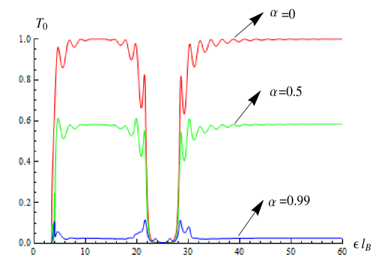
In Figure 6, the transmission coefficients $T_{l}$ is shown versus the energy $\epsilon l_{B}$. The quantity $k_{y}l_{B}=m^{\ast}$ plays a very important role in the transmission of Dirac fermions via the obstacles created by the series of scattering potentials, because it is associated with an effective mass of the particle and hence determines the threshold for the allowed energies. However, the application of the magnetic field in the intermediate zone where the barrier oscillates sinusoidally around $v$ with amplitude $v_{j}$ and frequency $\varpi$ seems to reduce this effective mass to $(k_{y}l_{B}-l\varpi l_{B})$ in the incidence region while it increases it to $(k_{y}l_{B}+\frac{d}{l_{B}}-l\varpi l_{B})$ in the transmission region. The allowed energies are then determined by the greater effective mass, namely $\epsilon l_{B}\geq k_{y}l_{B}+\frac{d}{l_{B}}-l\varpi l_{B}$.

Figure 7: (Color online) Graphs depicting the transmission $T_{0}$ as a function of potential $vl_{B}$ for the monolayer graphene barriers with $\alpha=0$, $\epsilon l_{B}=25$, $k_{y}l_{B}=2$ and $\frac{d}{l_{B}}=0,02$ (red), $\frac{d}{l_{B}}=1.2$ (green) and $\frac{d}{l_{B}}=5$ (blue).

In Figure 7, one can see that the transmission is depending on $vl_{B}$ for $\alpha=0$. This shows us how although the transmission is complete for small widths of the potential and how a bowl, corresponding a total reflection in the vicinity of the energy of propagation, is wider in terms of the width of the potential which behaves as the effective mass is added.

Figure 8: (Color online) Transmission probability of electrons for central band and first few sidebands for $\alpha=0.99$ along with that for static barrier as a function of the barrier width $\epsilon l_{B}=5$, $vl_{B}=12$, $\varpi l_{B}=2$ and $k_{y}l_{B}=1$.

Figure 9: (Color online) Transmission probability of electrons for central band and first few sidebands for a- $\alpha=0.4$ and b- $\alpha=0.99$ along with that for static barrier as a function of the barrier width $d=1l_{B}$, $vl_{B}=12$, $\epsilon l_{B}=5$ and $\varpi l_{B}=0.5$.

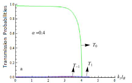
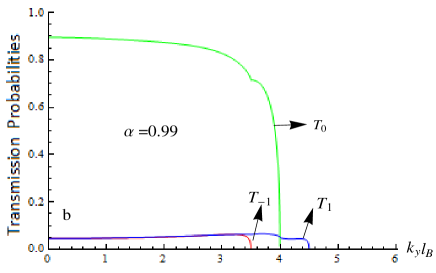
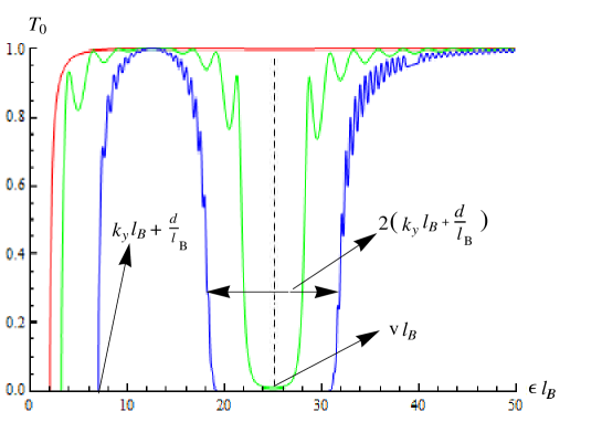
Both of Figures 8 and 9 show the effects of $\frac{d}{l_{B}}$ and $k_{y}l_{B}$ are similar to the point of view of the limitations of permitted transmissions. We observe that the two parameters $\frac{d}{l_{B}}$ and $k_{y}l_{B}$ act as an effective mass respecting, respectively, the two following relations: $k_{y}l_{B}\leq\epsilon l_{B}-\frac{d}{l_{B}}+l\varpi l_{B}$ and $\frac{d}{l_{B}}\leq\epsilon l_{B}-k_{y}l_{B}+l\varpi l_{B}$. It should be noted that the sum of the transmissions of different modes $(l=-1,0,1)$ would never exceeds the unit.

Figure 10: (Color online) Graphs depicting the transmission probability for central band $T_{0}$ and first sidebands $T_{\pm 1}$ as a function of potential $vl_{B}$ for the monolayer graphene barriers $d=\{0.05l_{B},1.6l_{B},2.4l_{B},3.2l_{B}\}$, with $\alpha=0.99$, $\epsilon l_{B}=25$, $\varpi l_{B}=2$ and $k_{y}l_{B}=2$.

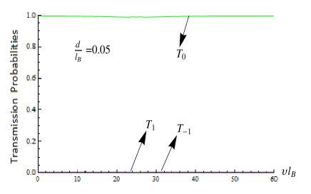
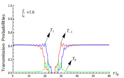
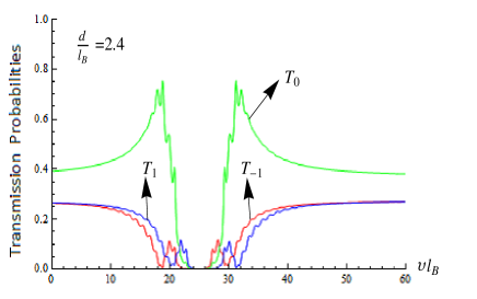
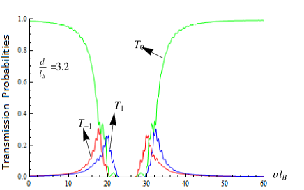
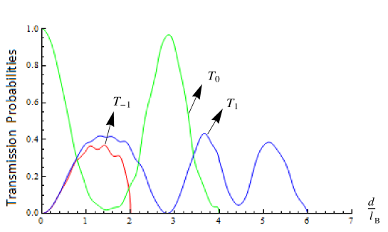
From Figure 10, one can see that the evolution of the central transmission band and the two lateral bands is depending on the width from the single oscillating potential over time accompanied by a magnetic field, and recognizes four different important phases depending on the desired applications. The first phase starts for very small widths which was the dominance of the central band that is significantly large and that begins with a total transmission whatever the applied potential. The second phase comes in second order in which it was the dominance of the two side bands each of which is symmetrical to the other relative to an axis of symmetry located at the potential corresponding to propagation energy. The third phase is similar to the second but with dominance changing between the central strip and the lateral strips retaining the sum between the different transmissions found less than or equal to unity. In the last phase, the central strip recovers its dominance but this faith latter with a total reflection from the turns predicted axis of symmetry and a total distance of the transmission axis. The transmissions of the two lateral strips are placed close to the axis of symmetry in which central transmission is strictly between zero and one such that the sum of all transmissions does not exceed the transmission unit and each sideband becomes symmetrical relative to the opposite to the axis of symmetry.

Figure 11: (Color online) Graphs depicting the transmission probability for central band $T_{0}$ and first sidebands $T_{\pm 1}$ as function of energy $\epsilon l_{B}$ for the monolayer graphene barriers $d=\{0.5l_{B},1.2l_{B},2.4l_{B},3l_{B}\}$, with $\alpha=0.99$, $vl_{B}=25$, $\varpi l_{B}=2$ and $k_{y}l_{B}=2$.

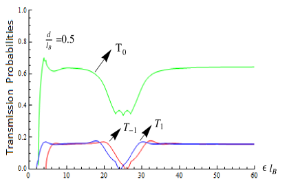
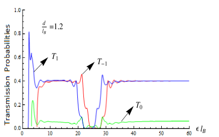
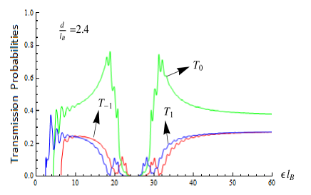
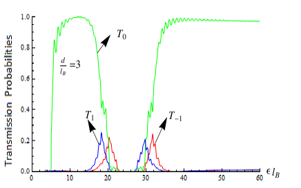
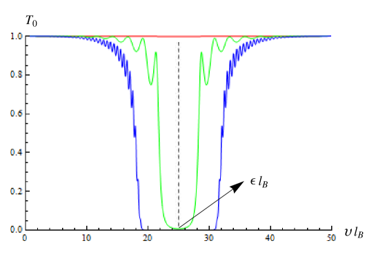
Figure 11 tells us that in the same way the evolution of the same transmissions, depending on the energy, are as before. This faith by complying forbidden energies below the effective mass, namely $\epsilon l_{B}\geq k_{y}l_{B}+\frac{d}{l_{B}}-l\varpi l_{B}$.

7 Total transmission probability

For static barrier, we know that there is only one transmission probability, which is function of the barrier width. Whereas in the oscillating barrier the total transmission probability for energy $\epsilon$ is given by the sum over all modes $l$

$$T=\sum_{l=-\infty}^{l=+\infty}T_{l}.$$ (124)

In the forthcoming analysis, let us choose the parameters characterizing our system in such manner that the lateral bands from $l=\pm 2$ and so on switch off quickly and the sum of the partial transmissions

$$T^{{}^{\prime}}=\sum_{-N}^{N}T_{l}$$ (125)

converges significantly to

$$T^{{}^{\prime}}=T_{-1}+T_{0}+T_{1}$$ (126)

which represent from now the total transmission of all system modes. With this we will see how the results presented for each mode previously in different figures for $T_{0}$ and $T_{\pm 1}$ will be summed up to get the total transmission plots.

Figure 12: (Color online) a-graphs depicting the transmission probability for central band $T_{0}$ and first sidebands $T_{\pm 1}$ as a function of energy $\epsilon l_{B}$ and b-Graphs depicting the transmission probability for $T^{{}^{\prime}}=T_{-1}+T_{0}+T_{1}$ as a function of energy $\epsilon l_{B}$ for the monolayer graphene barriers. $\frac{d}{l_{B}}=3$, with $\alpha=0.99$, $vl_{B}=25$, $\varpi l_{B}=2$ and $k_{y}l_{B}=2$.

Figure 13: (Color online) a-graphs depicting the transmission probability for central band $T_{0}$ and first sidebands $T_{\pm 1}$ as a function of potential $vl_{B}$ and b-Graphs depicting the transmission probability for $T^{{}^{\prime}}=T_{-1}+T_{0}+T_{1}$ as a function of potential $vl_{B}$ for the monolayer graphene barriers. $\frac{d}{l_{B}}=3.2$, with $\alpha=0.99$, $\epsilon l_{B}=25$, $\varpi l_{B}=2$ and $k_{y}l_{B}=2$.

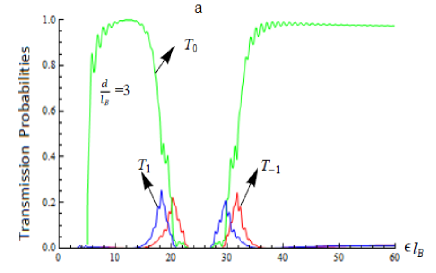
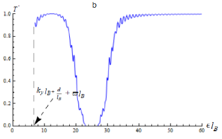
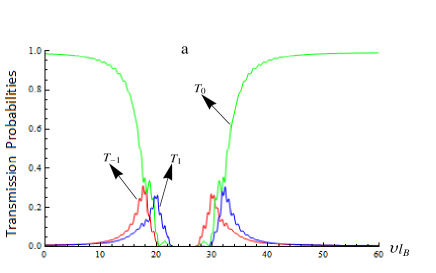
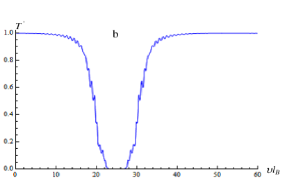
Figure 12 presents $T^{\prime}$ versus the energy $\epsilon l_{B}$. We notice that the allowed energies are determined by the greater effective mass, namely $\epsilon l_{B}\geq k_{y}l_{B}+\frac{d}{l_{B}}+N\varpi l_{B}$. It is clearly see that the $T_{0}$ behavior corresponding central band is much more dominated than other two remaining bands.

In Figure 13, we present $T^{\prime}$ in terms of the potential width $vl_{B}$. To make a clear comparison with former analysis, we pick up the last Figure 10 and give the plot below with the same conditions. This show clearly that we have a fully transmission behavior that summing up all that obtained for $T_{-1}$, $T_{0}$ and $T_{1}$.

8 Conclusion

We have considered Dirac Fermions in graphene subjected to an external magnetic field and time-dependent potential. The solutions of the energy spectrum were obtained for three regions composing the graphene sheet in terms of different physical parameters and the Bessel functions. The obtained eigenvalues are rich so that we have seen that absorbing energy quantum $\varpi$ produces interlevel transitions. Because of the Pauli principle an electron with energy $\epsilon$ can absorb an energy quantum $\varpi$ if only the state with energy $\epsilon+\varpi$ is empty.

Subsequently, we have studied the effect of both oscillating field and applied magnetic field on the electron transport through a single barrier. The time dependent oscillating barrier height generates additional sidebands at energies $\epsilon+l\hbar\omega$ $(l=0,\pm 1,\cdots)$ in the transmission probability due to photon absorption or emission. We have observed that perfect transmission probability at normal incidence (Klein tunneling) persist for harmonically driven single barrier.

We have investigate how the transmission probability is affected by various physical parameters, in particular the barrier width, energy and oscillation frequency. Thus our numerical results support the assertion that quantum interference has an important effect on particle tunneling through a time-dependent graphene-based single barrier. Since most optical applications in electronic devices are based on interference phenomena then we expect that the results of our computations might be of interest to designers of graphene-based electronic devices.

References

- [1] A. K. Geim and K. S. Novoselov, Nat. Mater. 6, 183 (2007).
- [2] K. S. Novoselov, A. K. Geim, S. V. Morozov, D. Jiang, Y. Zhang, S. V. Dubonos, I. V. Grigorieva and A. A. Firsov, Science 306, 666 (2004).
- [3] A. H. Castro Neto, F. Guinea, N. M. R. Peres, K. S. Novoselov and A. K. Geim, Rev. Mod. Phys. 81, 109 (2009).
- [4] A. H. Dayem and R. J. Martin, Phys. Rev. Lett. 8, 246 (1962).
- [5] P. K. Tien and J. P. Gordon, Phys. Rev. 129, 647 (1963).
- [6] M. Moskalets and M. Buttiker, Phys. Rev. B 66, 035306 (2002).
- [7] M. Wagner, Phys. Rev. A 51, 798 (1995).
- [8] M. Wagner, Phys. Rev. B 49, 16544 (1994).
- [9] F. Grossmann, T. Dittrich, P. Jung, P. Hanggi, Phys. Rev. Lett. 67, 516 (1991).
- [10] M. Ahsan Zeb, K. Sabeeh and M. Tahir, Phys. Rev. B 78, 165420 (2008).
- [11] P. Jiang, A. F. Young, W. Chang, P. Kim, L. W. Engel and D. C. Tsui, Appl. Phys. Lett. 97, 062113 (2010) and references therein.
- [12] H. L. Calvo, H. M. Pastawski, S. Roche and L. E. F. Foa Torres, Appl. Phys. Lett. 98, 232103 (2011).
- [13] P. San-Jose, E. Prada, H. Schomerus and S. Kohler, Appl. Phys. Lett. 101, 153506 (2012).
- [14] S. E. Savel’ev and A. S. Alexandrov, Phys. Rev. B 84, 035428 (2011).
- [15] S. E. Savel’ev, W. Hausler and P. Hanggi, Phys. Rev. Lett. 109, 226602 (2012).
- [16] T. L. Liu, L. Chang and C. S. Chu, Phys. Rev. B 88, 195419 (2013).
- [17] M. V. Fistul and K. B. Efetov, Phys. Rev. Lett. 98, 256803 (2007).
- [18] E. Grichuk and E. Manykin, Eur. Phys. J. B 86, 210 (2013).
- [19] S. E. Savel’ev, W. Hausler and P. Hanggi, Eur. Phys. J. B 86, 433 (2013).
- [20] L. Gammaitoni, P. Hanggi, P. Jung and F. Marchesoni, Rev. Mod. Phys. 70, 223 (1998).
- [21] Luo-Luo Jiang, Liang Huang, Rui Yang and Yin-Cheng Lai, Appl. Phys. Lett. 96, 262114 (2010).
- [22] A. Pototsky, F. Marchesoni, F. V. Kusmartsev, P. Hanggi and S. E. Savel’ev, Eur. Phys. J. B 85, 35 (2012).
- [23] A. De Martino, L. DellAnna and R. Egger, Phys. Rev. Lett. 98, 066802 (2007).