Generalized epidemic process on modular networks

Abstract

Social reinforcement and modular structure are two salient features observed in the spreading of behavior through social contacts. In order to investigate the interplay between these two features, we study the generalized epidemic process on modular networks with equal-sized finite communities and adjustable modularity. Using the analytical approach originally applied to clique-based random networks, we show that the system exhibits a bond-percolation type continuous phase transition for weak social reinforcement, whereas a discontinuous phase transition occurs for sufficiently strong social reinforcement. Our findings are numerically verified using the finite-size scaling analysis and the crossings of the bimodality coefficient.

I Introduction

Numerous studies have discussed epidemics on various types of networks Dorogovtsev et al. (2008); Barrat et al. (2008); Havlin and Cohen (2010), but the epidemics of behaviors in societies remains less understood. The latter phenomenon has two features that make it more complex than the former. First, there is social reinforcement: Each individual has the memory of previous social interactions, so that a new behavior is more easily transmitted from an approving neighbor when it has been affirmed by a greater number of social connections Centola and Macy (2007); Centola (2010); [Thereexistsadifferentperspectiveonthisconcept; whichconsidersmemorylesssocialreinforcement.See]DeDomenico2013. Second, human societies usually have highly-clustered modular structures Granovetter (1978). Developing proper mathematical devices to deal with these two features has been a theoretical challenge. In this paper, we present a model for which this problem can be successfully addressed so that the phase transition properties of behavioral epidemics can be analytically predicted.

Previous studies have modeled social reinforcement in several different ways. For example, each node may require a minimum number of approving neighbors to adopt a behavior Centola and Macy (2007); Granovetter (1978); Watts (2002); Centola et al. (2007). Alternatively, an individual may go through a series of intermediate “awareness” levels before the final adoption Krapivsky et al. ; Zheng et al. (2013). Otherwise, the probability of adoption may change for each recommendation received from an additional approving neighbor Lü et al. (2011). The generalized epidemic process (GEP) belongs to the last type, in which the probability of adoption is an arbitrary function of the number of previous recommendations Janssen et al. (2004); Dodds and Watts (2004); Bizhani et al. (2012). The GEP on locally tree-like random networks was analytically solved Bizhani et al. (2012) using a self-consistency equation argument analogous to the derivation of bond percolation threshold on random networks Newman et al. (2001); Newman (2002). The solution revealed that the GEP exhibits a bond-percolation type continuous phase transition for weak social reinforcement, which changes to a discontinuous transition for sufficiently strong social reinforcement. Whether the GEP on more realistic highly clustered networks has similar properties is an interesting problem, since the previous self-consistency equation argument assumes locally tree-like structure and cannot be directly applied to such clustered systems.

While previous works about behavioral epidemics on highly clustered networks Centola and Macy (2007); Centola (2010); Centola et al. (2007); Lü et al. (2011) primarily dealt with the small-world networks Watts and Strogatz (1998), we prefer to focus on the modular networks consisting of highly-clustered communities joined by random inter-community links Girvan and Newman (2002). Such networks capture three crucial properties of social networks at once: clustering, modularity, and small worldness. Besides, such modular networks are structurally very similar to clique-based random networks, whose cascading properties were recently shown to be analytically tractable by a variant of self-consistency equation argument Gleeson (2009); Hackett and Gleeson (2013). Keeping these considerations in mind, we have chosen the GEP on modular networks with equal-sized communities and adjustable proportions of intra- and inter-community links as the focus of our study. In order to reduce the complexity of the problem, we simplify the GEP so that the probability of adoption at and after the second approval is constant, as was the case in Janssen et al. (2004).

The rest of the paper is organized into four sections. In Sec. II, we define the modular network and the two different kinds (original and modified) of GEP used in our study. In Sec. III, we present an analytical approach to the original GEP, which predicts outbreak size, epidemic threshold, and the nature of phase transition. All predictions can be numerically verified. In Sec. IV, with the aid of the crossings of bimodality coefficient, we numerically show that the modified GEP shows the same transition nature despite the differences in the model details. Finally, we summarize our findings and discuss their possible implications in Sec. V.

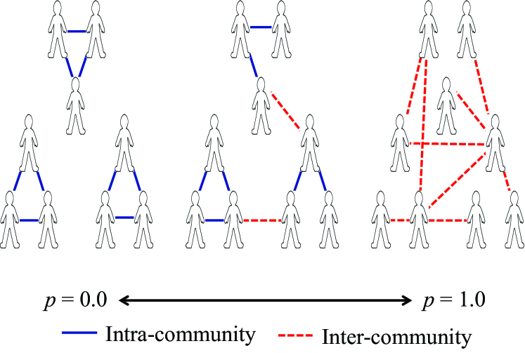
Figure 1: (Color online) Schematic illustration of modular networks for various $p$: The network at $p=0$ consists of $N=12$ nodes partitioned into communities of size $c=3$. As $p$ increases from $0$ to $1$, the disconnected cliques gradually changes via a series of modular structures to the ER network.

II Model

II.1 Modular network

We consider a modular network of $N$ nodes, which consists of predefined communities with $c$ nodes each. The total number of links is fixed so that the average degree is exactly $c-1$. A fraction $p$ of the links connect random pairs of nodes, while the others are all intra-community ties. Self-loops and parallel links are forbidden. If $p=0$, the network has disconnected cliques of size $c$, whereas $p=1$ corresponds to an Erdős–Rényi (ER) network. Thus, by varying $p$ between $0$ and $1$, we can adjust the modularity of the network (see Fig. 1 for a schematic illustration of the effect of $p$). This network is very similar to (but not exactly the same as) the benchmark modular network used in Girvan and Newman (2002). We define the asymptotic limit of this network as the limit of $N\to\infty$ with $c$ kept finite. In this limit, $p$ is effectively the fraction of inter-community ties since a random pair of nodes is far more likely to belong to different communities [$O(N^{2})$ pairs] than to the same community [$O(N)$ pairs].

II.2 Generalized epidemic process (GEP)

In the context of behavioral epidemics, the GEP can be defined as an epidemic process in which the probability of a node adopting the spreading behavior depends on the number of previous unsuccessful attempts to persuade the node Janssen et al. (2004); Bizhani et al. (2012). In the most general case, the probability of adoption at the $n$-th attempt can be denoted by $\lambda_{n}$. In the beginning, the behavior is adopted by a single random node, which is active in the sense that it tries to spread the behavior to its neighbors. At every instant, one randomly chosen active node tries to persuade all its neighbors simultaneously, with the probability of success given by $\lambda_{n}$; any persuaded neighbor adopts the behavior and becomes active. After then, the node deactivates and no longer participates in the dynamics, losing interest in spreading the behavior. This process continues until the system runs out of active nodes. If $R$ nodes adopt the behavior in the end, we call $R$ the outbreak size and $R/N$ the fractional outbreak size.

In the simplest case when all probabilities of adoption are equal ($\lambda_{1}=\ldots=\lambda_{\infty}=\lambda$), the process reduces to the well-known susceptible-infected-recovered (SIR) model Newman (2002), which lacks social reinforcement. We focus on the case minimally more sophisticated than the SIR model, where $\lambda_{1}=\lambda$ and $\lambda_{2}=\cdots=\lambda_{\infty}=T$. Here $\lambda$ represents the inherent strength of the behavior, while $T$ indicates the modified strength of the behavior resulting from the memory of social interactions. When $T>\lambda$, multiple recommendations synergistically enhance the probability of adoption. If $T<\lambda$, multiple recommendations have inhibitory effects on the spreading of behavior. We note that $T<\lambda$ can also be interpreted as the case when the spreading occurs in an explorative way rather than an exploitative way, always preferring to spread through the sites that have been contacted fewer times Pérez-Reche et al. (2011).

For a given set of parameters $c$, $p$, and $T$, there exists an epidemic threshold $\lambda_{c}$ such that $R/N$ can converge to a nonzero value as $N\to\infty$ only for $\lambda>\lambda_{c}$. This phenomenon is called the epidemic transition, which can be interpreted as an absorbing phase transition whose order parameter is the largest possible asymptotic limit of $R/N$. Analytic predictions of this order parameter is explained in Sec. III.

II.3 Modified GEP

In the original GEP, an active node tries to persuade its neighbors. In reality, the spreading of behavior may occur in a slightly different way, in which a randomly chosen susceptible node observes its neighbors and decides whether to adopt the behavior depending on the number of approving neighbors. We require that the node does not update its state when the number of approving neighbors has not changed since the last observation. Thus, the process stops when there is no node that can observe any change in its neighborhood. This process is different from the original GEP in that the probability of adoption does not always change sequentially from $\lambda$ to $T$; depending on the observed number of approving neighbors, the first probability of adoption experienced by the node may well be $T$ rather than $\lambda$. We call this process the modified GEP, whose properties are numerically investigated in Sec. IV.

III Analysis of original GEP

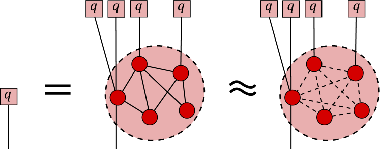
Figure 2: (Color online) Schematic illustration of the self-consistency equation approach to the GEP on modular networks. A modular network is equivalent to a clique-based network sharing the same value of $c$ but with every intra-clique equally disconnected with probability $p$. Since all external neighbors are similar and independent of each other, a self-consistency equation can be obtained for the probability $q$ that an external neighbor adopts the spreading behavior.

This section presents a self-consistency equation approach to the GEP on modular networks, from which the asymptotic limit of $R/N$ can be derived. The approach, originally developed for locally tree-like networks Newman (2002); Bizhani et al. (2012), was recently generalized to clique-based random networks Gleeson (2009); Hackett and Gleeson (2013). We describe how this generalized approach can be adapted to modular networks.

Consider a clique-based random network that consists of cliques of size $c$ and some additional links that connect random pairs of nodes belonging to different cliques. The number of these inter-clique links is such that each node has on average $p(c-1)$ external neighbors belonging to the other cliques in addition to $c-1$ internal neighbors in the same clique. Then, the degree distribution of the network satisfies

$$P(k)=\begin{cases}\frac{\left[p(c-1)\right]^{k-c+1}}{(k-c+1)!}e^{-p(c-1)}&\text{for $k\geq c-1$}\\ 0&\text{for $k<c-1$}.\end{cases}$$ (1)

We denote by $F_{l,j}$ the probability that a node has adopted the behavior by the time $l$ internal and $j$ external neighbors have adopted it. For the sake of simplicity, we assume $T=\lambda$ for the moment. For clique-based random networks, $F_{l,j}$ can be written as $F_{l+j}$ because both internal and external neighbors contribute equally to its value Hackett and Gleeson (2013). More specifically, each neighbor fails to persuade the node with probability $1-\lambda$, thus

$$F_{l+j}=1-(1-\lambda)^{l+j}.$$ (2)

However, in modular networks, on average a fraction $p$ of the inter-clique links are actually disconnected. To account for these nonexistent links, the probability that an internal neighbor fails to persuade the node must be put equal to $p+(1-p)(1-\lambda)$, where $p$ represents the absence of a link and $(1-p)(1-\lambda)$ is the failure to persuade the node despite the presence of a link. Therefore,

$$F_{l,j}=1-\left[p+(1-p)(1-\lambda)\right]^{l}(1-\lambda)^{j}.$$ (3)

Returning to the case of $T\neq\lambda$, any $(1-\lambda)^{n}$ with $n\geq 2$ must be replaced with $(1-\lambda)(1-T)^{n-1}$. Then, Eq. (3) is rewritten as

$$F_{l,j}=1 -[1-(1-p)T]^{l}(1-T)^{j-1}(1-\lambda)$$

$$+\delta_{j,0}\frac{T-\lambda}{1-T}p^{l},$$ (4)

which is the expression we use to describe the GEP on modular networks. We note that the use of Eqs. (1) and (III) is the only change required for making the approach of Gleeson (2009); Hackett and Gleeson (2013) applicable to modular networks. The rest of the derivation is essentially the same as that given by Hackett and Gleeson (2013), which is reviewed in the following for the sake of completeness.

We denote by $q$ the probability that a node at an end of a randomly chosen inter-clique link ends up adopting the behavior through one of the $k-1$ excess links other than the inter-clique link chosen in the beginning. Suppose that the probability of $j$ among $k-c$ external neighbors ($l$ among $c-1$ internal neighbors) adopting the behavior before the behavior spreads to the node is given by $B_{j}^{k-c}(q)$ [$R_{l}^{c-1}(q)$]. Then $q$ satisfies the self-consistency equation

$$q=\sum_{k=1}^{\infty}P^{\prime}(k)\sum_{j=0}^{k-c}\sum_{l=0}^{c-1}B_{j}^{k-c}(q)R_{l}^{c-1}(q)F_{l,j},$$ (5)

where

$$P^{\prime}(k)=\frac{(k-c+1)P(k)}{p(c-1)}=P(k-1)$$ (6)

is the degree distribution of a node at an end of a randomly chosen inter-clique link (see Fig. 2 for a schematic illustration of this self-consistency equation). Similarly, the probability that a randomly chosen node adopts the behavior through one of its $k$ links is given by

$$\lim_{N\to\infty}\frac{R}{N}=\sum_{k=0}^{\infty}P(k)\sum_{j=0}^{k-c+1}\sum_{l=0}^{c-1}B_{j}^{k-c+1}(q)R_{l}^{c-1}(q)F_{l,j}.$$ (7)

From Eqs. (5) and (6), it is clear that

$$q=\lim_{N\to\infty}\frac{R}{N}.$$ (8)

Thus, solving Eq. (5) for $q$ automatically yields the asymptotic limit of the fractional outbreak size $R/N$.

It is very straightforward to obtain $B_{j}^{k-c+1}(q)$, since the locally tree-like structure of inter-clique links implies that each external neighbor adopts the behavior with independent and identical probability equal to $q$. Thus, $B_{j}^{k-c+1}$ is given by the binomial distribution

$$B_{j}^{k-c}(q)=\binom{k-c}{j}q^{j}(1-q)^{k-c-j}.$$ (9)

On the other hand, calculating $R_{l}^{c-1}(q)$ is far more tedious due to the strong interdependence arising from local clustering. We must consider every possible way to spread the behavior among $l$ internal neighbors (while keeping the node itself unaffected) in a single or multiple steps of cascades. An interested reader is referred to Hackett and Gleeson (2013) for the detailed derivation, and here we simply describe the final result:

$$R_{l}^{c-1}(q)=\sum_{(l_{i})}\prod_{i=1}^{v}B_{l_{i}}^{n_{c,i}}(\theta_{c,i}).$$ (10)

The summation is over all possible integer sequences $(l_{i})_{i=1}^{v}$ of variable length $v$ satisfying $l=\sum_{i=1}^{v}l_{i}$ and $l_{i}>0$ except that $l_{v}=0$ for $l<c-1$ [Ifweexcludethezeroelements; thissetofall$(l_i)$isjustthesameasthesetofallcompositionsoftheinteger$l$; whichhasbeenextensivelystudiedincombinatorics.See]Heubach2009. Also note that, adopting the simplifying notation $l_{0}=0$ and $m_{i}=\sum_{j=0}^{i}l_{j}$,

$$n_{c,i}=c-1-m_{i-1}$$ (11)

and

$$\theta_{c,i}=\begin{cases}\frac{G_{m_{i-1}}^{c-1}(q)-G_{m_{i-2}}^{c-1}(q)}{1-G_{m_{i-2}}^{c-1}(q)}&\text{if $i\geq 2$}\\ G_{0}^{c-1}(q)&\text{if $i=1$},\end{cases}$$ (12)

where $G_{m}^{c-1}(q)$ denotes the probability that a single member of the clique has adopted the behavior by the time $m$ other members have adopted the behavior:

$$G_{m}^{c-1}(q) =\sum_{k=0}^{\infty}P(k)\sum_{j=0}^{k-c+1}B_{j}^{k-c+1}(q)F_{m,j}$$

$$=1-\frac{1-\lambda}{1-T}[1-(1-p)T]^{m}e^{-(c-1)pqT}$$

$$\quad+\frac{T-\lambda}{1-T}p^{m}e^{-(c-1)pq}.$$ (13)

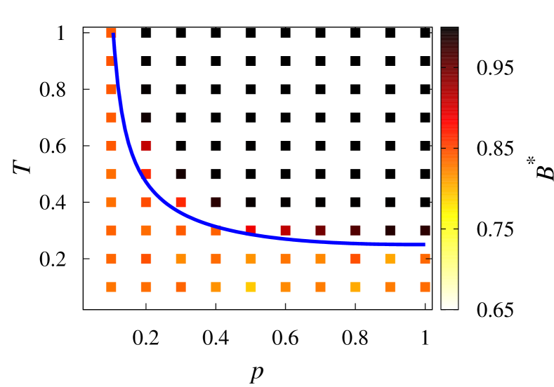
Figure 3: (Color online) Diagram of transition nature for $c=6$. The solid line indicates the tricritical line of the original GEP predicted by the analytical approach, while the gradation of shades indicates the crossing point values of the bimodality coefficient $B^{*}$ for the modified GEP numerically obtained at $N=768000$ and $1536000$. The curvature of the predicted line is qualitatively similar to that of the observed boundary.

From Eqs. (7), (8), and (III), the self-consistency equation can be rewritten as

$$q=H(q)\equiv\sum_{l=0}^{c-1}R_{l}^{c-1}(q)G^{c-1}_{l}(q).$$ (14)

This equation always has a solution at $q=0$, which corresponds to the localized spreading of behavior. An epidemic outbreak is possible only if Eq. (14) has a nonzero solution. In order to check this possibility, we may examine a Taylor expansion of Eq. (14) given by

$$H(q)-q =[H^{\prime}(0)-1]q+\frac{H^{\prime\prime}(0)}{2}q^{2}+O(q^{3})$$

$$=a(\lambda-\lambda_{c})q+\frac{H^{\prime\prime}(0)}{2}q^{2}+O[q^{3}+q(\lambda-\lambda_{c})^{2}]$$

$$=0,$$ (15)

where $H^{\prime}(0)=1$ at $\lambda=\lambda_{c}$ and $a\equiv\partial H^{\prime}(0)/\partial\lambda|_{\lambda=\lambda_{c}}$ is a positive coefficient.

For $H^{\prime\prime}(0)<0$, Eq. (III) implies that $q=0$ is the only solution for $\lambda\leq\lambda_{c}$, and a nonzero solution becomes available for $\lambda>\lambda_{c}$. When $\lambda$ is only slightly larger than $\lambda_{c}$, the nonzero solution satisfies $q\sim(\lambda-\lambda_{c})^{\beta}$ with the critical exponent given by the mean-field value $\beta=1$. The other critical exponents cannot be determined from Eq. (14) alone, for they are dependent on the size distribution of finite outbreaks ($R\ll N$) Havlin and Cohen (2010), whose properties are not well described by Eq. (14). Nonetheless, we expect them to be equal to the mean-field values because, for finite outbreaks, the effect of $T$ is limited to local communities and would not affect the scale-invariant critical properties. Thus, whenever $H^{\prime\prime}(0)<0$, the epidemic transition would not be distinguishable from the ordinary bond percolation transition.

By contrast, if $H^{\prime\prime}(0)>0$, the transition becomes discontinuous. The boundary between the two different types of transitions, or the tricritical point $(\lambda_{t},\,T_{t})$, is given by

$$H^{\prime}(0)=1,\quad H^{\prime\prime}(0)=0.$$ (16)

For the special case of ER networks ($p=1$), Eq. (16) yields

$$\lambda_{t}=1/(c-1),\quad T_{t}=\lambda_{t}/(1-\lambda_{t}),$$ (17)

which confirms the result of Bizhani et al. (2012) obtained for locally tree-like networks. If $p<1$, the tricritical point $T_{t}$ cannot be written in a simple form, but it can still be calculated by numerically solving Eq. (16). The predicted relationship between $p$ and $T_{t}$ is shown by the thick curve in Fig. 3. This curve separates the region of discontinuous transition (above the curve) from that of continuous transition (below the curve).

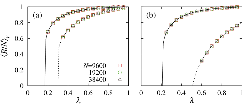
Figure 4: (Color online) Comparison between analytical predictions (lines) and numerical estimations (symbols) of the right-peak average $\langle R/N\rangle_{r}$, which indicates the nonzero fractional outbreak size. They give consistent results for the GEP on both (a) clique-based networks ($c=6$, $p=0.2$, $T=0.7$ for solid line and $c=3$, $p=0.8$, $T=0.7$ for dashed line) and (b) modular networks ($c=6$, $p=0.2$, $T=0.7$ for solid line and $c=3$, $p=0.8$, $T=0.7$ for dashed line).

The analytical approach explained in this section can be numerically verified. The distribution of $R/N$ obtained from simulations consists of two clearly separable peaks for $\lambda$ sufficiently larger than $\lambda_{c}$. Since the left peak is very close to $R/N=0$, only the right peak corresponds to the nonzero fractional outbreak size predicted by the analytical approach. Thus, we may use the right-peak average of $R/N$, denoted by $\langle R/N\rangle_{r}$, as an estimator of the nonzero fractional outbreak size. A comparison between this estimator (symbols) and the prediction (lines) is shown in Fig. 4. As $N$ increases, the former approaches the latter for both clique-based [Fig. 4(a)] and modular [Fig. 4(b)] networks, which is a strong evidence for the validity of the theory.

The estimator $\langle R/N\rangle_{r}$ can be measured reliably only when the right peak is separable from the left peak and contains sufficiently many samples. For this reason, the epidemic threshold $\lambda_{c}$ cannot be directly verified by $\langle R/N\rangle_{r}$. As an alternative indicator of $\lambda_{c}$, we use the crossing of bimodality coefficient, which is described in details in Sec. IV. For the moment, we simply note that the estimated $\lambda_{c}$ is consistent with the prediction, as shown for the case of $\lambda=T$ in Fig. 5.

IV Analysis of modified GEP

While the analytical approach described in Sec. III has been shown to be accurate for the ordinary GEP, it is inaccurate for the modified GEP. Since multiple persuasion attempts in the former process can be treated as a single observation event in the latter, the modified GEP always has a fewer number of updates. Thus, its outbreak size must be smaller than that of the ordinary GEP, and consequently its epidemic threshold would be larger. However, we may still check whether these differences lead to any notable changes in the nature of phase transition, namely its (dis)continuity and critical exponents. For this purpose, we perform numerical simulations of the modified GEP on modular networks. Provided that $p$ is high enough to ensure the existence of a percolating giant cluster, the qualitative properties of the model were checked to be largely invariant with respect to the choice of $c$ and $p$. Therefore, without loss of generality, we present the results for $c=6$ and $p=0.2$ unless otherwise noted.

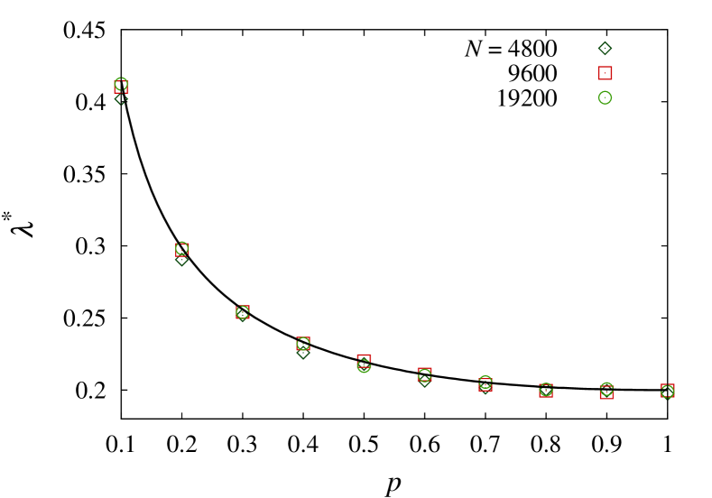
Figure 5: (Color online) Comparison of $\lambda^{*}$ (symbols) obtained from the crossings of $B(\lambda)$ with the analytical prediction of $\lambda_{c}$ (line) in the absence of social reinforcement ($T=\lambda$) for the GEP on modular networks with $c=6$. The prediction is in good agreement with the numerical results.

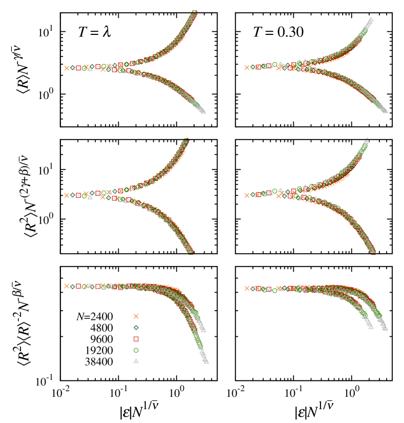
Figure 6: (Color online) FSS of moments of outbreak size $R$ for the modified GEP with $c=6$ and $p=0.2$. The notation $\epsilon\equiv\lambda/\lambda_{c}-1$ is used. The data are obtained from $10^{5}$ samples. When social reinforcement is absent ($T=\lambda$, $\lambda_{c}=0.3283$; left panel) or weak ($T=0.30$, $\lambda_{c}=0.3384$; right panel), the data are well collapsed with $\beta=1$, $\gamma=1$, and $\bar{\nu}=3$ as expected.

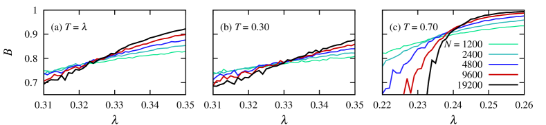
Figure 7: (Color online) Bimodality coefficient $B(\lambda)$ of the outbreak size distribution near $\lambda_{c}$ for the modified GEP with $c=6$ and $p=0.2$, measured for $10^{5}$ samples. The slope of the curve increases with $N$, making a series of crossings that stay around a value much smaller than $1$ for (a) the absence of social reinforcement ($T=\lambda$) and (b) weak social reinforcement ($T=0.30$), while it is close to $1$ for (c) strong social reinforcement ($T=0.70$).

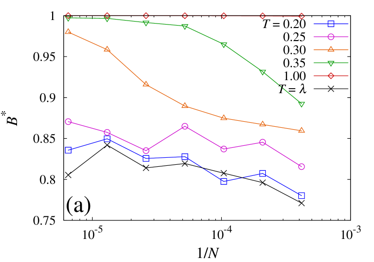
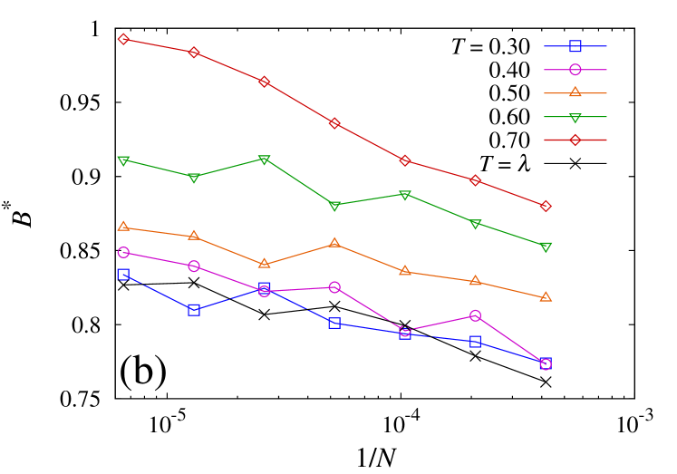
Figure 8: (Color online) The rightmost crossings $B^{*}(N)$ of two $B(\lambda)$ curves for system sizes $N$ and $2N$, obtained from $10^{5}$ runs of the modified GEP with $c=6$. Results for (a) $p=1.0$ and (b) $p=0.2$ are shown separately. Interpreting the asymptotic limit of $B^{*}$ as $B(\lambda_{c})$, we observe that $B(\lambda_{c})$ approaches $1$ only for sufficiently strong social reinforcement.

We first estimate the critical exponents by the FSS analysis of the moments of outbreak size $R$. Using the notation $\epsilon\equiv(\lambda-\lambda_{c})/\lambda_{c}$, Fig. 6 shows that all data are well collapsed by the predicted FSS forms de Souza et al.

$$\langle R\rangle =N^{\gamma/\bar{\nu}}f(\left|\epsilon\right|N^{1/\bar{\nu}}),$$ (18)

$$\langle R^{2}\rangle =N^{(\beta+2\gamma)/\bar{\nu}}g(\left|\epsilon\right|N^{1/\bar{\nu}})$$ (19)

provided that social reinforcement is either absent ($T=\lambda$) or sufficiently weak ($T=0.30$) to yield continuous transitions. Here $\lambda_{c}$ is chosen to give the best collapse, and critical exponents are those of the mean-field bond percolation universality class ($\beta=1$, $\gamma=1$, $\bar{\nu}=3$). This shows that the critical properties of the modified GEP are likely to be the same as those of the original GEP.

Now we move on to check whether the modified GEP has both continuous and discontinuous transitions. In order to numerically determine the transition nature, we employ the bimodality coefficient $B$ SAS (2013) of the outbreak size distribution, which is defined as

$$B(\lambda)=\frac{\left\langle\left(\frac{R-\langle R\rangle}{\sigma}\right)^{3}\right\rangle^{2}+1}{\left\langle\left(\frac{R-\langle R\rangle}{\sigma}\right)^{4}\right\rangle},$$ (20)

where $\sigma\equiv\sqrt{\langle R^{2}\rangle-\langle R\rangle^{2}}$. This coefficient is equal to $1$ only for random variables with exactly two possible choices, such as Bernoulli trials or two delta peaks. It is smaller than $1$ for the other kinds of distributions Pearson (1921). In the case of the modified GEP, as $N\to\infty$, the bimodality coefficient at the transition point $B(\lambda_{c})$ converges to $1$ only for discontinuous transitions, whereas it approaches a smaller value determined by the outbreak size distribution $P(R)\sim R^{-\tau+1}$ (which is equivalent to the probability of a randomly chosen node belonging to a cluster of size $R$ in the original percolation problem de Souza et al. ) for continuous transitions:

$$B(\lambda_{c})=\frac{(4-\tau)(6-\tau)}{(5-\tau)^{2}}.$$ (21)

For the mean-field bond-percolation universality class, we have $\tau=5/2$, so $B(\lambda_{c})=0.84$.

As shown in Fig. 7, a pair of $B(\lambda)$ curves measured at different values of $N$ make some crossings. To estimate $\lambda_{c}$ and $B(\lambda_{c})$, we keep track of one of those crossings (say the rightmost one, to remove the ambiguity) as $N$ is successively increased by factors of $2$. Denoting by $(\lambda^{*},\,B^{*})$ the coordinates of the rightmost crossing, Figs. 5 and 8 show their behavior as $N$ is successively increased by factors of $2$. It seems that both $\lambda^{*}$ and $B^{*}$ converge to a limit, which can be interpreted as $\lambda_{c}$ and $B(\lambda_{c})$, respectively. The agreement between the predicted $\lambda_{c}$ and the estimator $\lambda^{*}$ for the original GEP shown in Fig. 5 supports this interpretation.

As shown for both $p=1$ [Fig. 8(a)] and $p=0.2$ [Fig. 8(b)], $B^{*}$ converges to values near $0.84$ when $T$ is sufficiently small or fixed equal to $\lambda$, which is to be expected from Eq. (21) and the mean-field bond-percolation critical exponents implied by Fig. 6. Meanwhile, for sufficiently large values of $T$, $B^{*}$ approaches very close to $1$, suggesting discontinuous transitions. Although the curves obtained at intermediate values of $T$ seemingly converge to values other than $0.84$ and $1$, we expect this to be a crossover phenomenon at finite size.

Based on these observations, we use $B^{*}$ obtained from two $B(\lambda)$ curves with sufficiently large values of $N$ as a proxy for the true $B(\lambda_{c})$. Figure 3 shows the $(p,T)$-dependence of $B^{*}$ obtained from $N=768000$ and $N=1536000$ by a gradation of shades. Both the dark region of discontinuous transition and the light region of continuous transition are observed, whose border shows a curvature similar to that of the tricritical line (solid curve) of the original GEP. Thus, despite the differences between the original and modified GEP, many properties related to the nature of phase transition remain similar.

V Summary and discussions

Using the self-consistency equation method adapted to clique-based random networks, we formulated an analytical approach to the generalized epidemic process (GEP) on modular networks, which describes the emergence of collective behavior through social contacts. The theory predicts that strong social reinforcement induces an abrupt epidemic outbreak (discontinuous transition), while weak social reinforcement leads to a gradual epidemic outbreak (continuous transition) whose critical exponents are those of the mean-field bond percolation universality class. We also obtained the mathematical condition [Eq. (16)] for the tricritical line that forms the boundary between the two different types of transition. These analytical predictions were numerically confirmed by tracking the crossings of the bimodality coefficient test. We also numerically showed that the modified GEP, in which the nodes observe rather than persuade others, exhibits the same transition nature despite the differences in the model details.

We note that the modularity parameter $p$ changes the positions of tricritical points only, leaving the nature of critical points and the existence of discontinuous transitions unaffected. Thus, the modular networks ($p<1$) turn out to have the same critical properties as those of the Erdős–Rényi (ER) networks ($p=1$). It is also notable that the tricritical point $T_{t}$ increases monotonically as $p$ is decreased. Since lowering $p$ increases clustering, it could have amplified the effect of social reinforcement so that $T_{t}$ is minimized at some $p<1$. Instead, $T_{t}$ is minimized at $p=1$, for which the clustering coefficient becomes zero. All these properties might be attributable to the fact that modular networks look similar to ER random networks when coarse grained, since clustering is localized to small communities and long-range inter-community links are randomly distributed. Reducing $p$ (i.e., removing inter-community links) is just equivalent to lowering the average degree of the coarse-grained ER random network, which merely raises the critical and the tricritical points. The critical exponents, which represent the scale-invariant properties Goldenfeld (1992), would remain unchanged as long as the coarse-grained structure of the network is essentially the same.

Finally, we comment on a few possible extensions of our study. First, we only considered the case when degree and community size distributions are very homogeneous, while both distributions tend to be heterogeneous for realistic networks Guimerà et al. (2003). Just as bond percolation on scale-free networks has a unique set of critical exponents, the critical properties of the GEP would be affected by such structural heterogeneity. Second, we discussed the GEP only from the phase transition perspective, but the model can also be studied from the viewpoint of optimization, as was done for small-world networks Lü et al. (2011). For example, what is the optimal value of $p$ that maximizes the outbreak size for given $\lambda$ and $T$? The analytical approach of Sec. III can also be applied to answer such questions. Lastly, the tricritical line predicted in our study might have its own critical properties, which can be addressed in future studies.