The photon magnetic moment problem revisited

Abstract

The photon magnetic moment for radiation propagating in magnetized vacuum is defined as a pseudo-tensor quantity, proportional to the external electromagnetic field tensor. After expanding the eigenvalues of the polarization operator in powers of $k^{2}$, we obtain approximate dispersion equations (cubic in $k^{2}$), and analytic solutions for the photon magnetic moment, valid for low momentum and/or large magnetic field. The paramagnetic photon experiences a red shift, with opposite sign than the gravitational one, which differs for parallel and perpendicular polarizations. It is due to the drain of photon transverse momentum and energy by the external field. By defining an effective transverse momentum, the constancy of the speed of light orthogonal to the field is guaranteed. We conclude that the propagation of the photon non-parallel to the magnetic behaves as if there is a quantum compression of vacuum or warp of space-time in an amount depending on its angle with regard to the field.

1 Introduction

We have shown in EliPRD that for a photon moving in a magnetic field $\mathbf{B}$, assumed constant and homogeneous (and for definiteness, taken along the $x_{3}$ axis, thus $|B_{3}|=B$, $B_{1}=B_{2}=0$ ), an anomalous magnetic moment defined as $\mu_{\gamma}=-\partial\omega/\partial B$ arises. This quantity has meaning, and can be defined only when the photon mass shell includes the radiative corrections, i.e., the magnetized photon self-energy, and calculated explicitly only after obtaining the solution of the photon dispersion equations shabad2 . It was shown that it is paramagnetic ($\mu_{\gamma}>0$), since it arises physically when the photon propagates, as due to the magnetic response of the virtual electron-positron pairs of vacuum, or vacuum polarization, under the action of $\mathbf{B}$, leading to vacuum magnetization. Thus, the photon embodies both properties of the free photon and of a magnetic dipole, which leads to consider it more as a quasi-photon, in analogy with the polariton of condensed matter physics polariton . Such properties are valid in the whole region of transparency, which is the region of momentum space where the photon self-energy, and in consequence, its frequency $\omega$, is real. This region is defined for transverse momentum $(\omega^{2}-k_{\parallel}^{2})^{1/2}\leq 2m$, where $\omega$, $k_{\parallel}$, are the photon frequency and momentum components along $\mathbf{B}$, and $m$ is the electron mass. In shabad2 it is shown that the quantities

$$z_{1} = (\mathbf{k}\cdot\mathbf{B})^{2}/\mathbf{B}^{2}-\omega^{2}=k_{\parallel}^{2}-\omega^{2},$$ (1)

$$z_{2} = (\mathbf{B}\times{\mathbf{k}})^{2}/\mathbf{B}^{2}$$

$$= \mathbf{k}^{2}-(\mathbf{k}\cdot\mathbf{B})^{2}/\mathbf{B}^{2}=k_{\perp}^{2},$$

are relativistic invariant variables for the photon propagating in the magnetic field $\mathbf{B}$, where $z_{1}+z_{2}=k^{2}$ is the square of the four-momentum vector $k_{\mu}$. In what follows we will use equally $z_{2}$ and $k_{\perp}^{2}$ when referring to the transverse momentum squared.

As pointed out in EliPRD , beyond that region, as the photon becomes unstable shabad2 for frequencies $\omega\geq 2m$ (and has a significant probability of decaying in electron-positron pairs), the photon magnetic moment loses meaning if considered independent of the magnetic moment produced by the electron-positron background. Let us remark that the case studied in EliPRD , shabad2 is based on the hypothesis of a constant and homogeneous magnetic field defined by the invariants $\textsf{F}={\cal F}_{\mu\nu}^{2}=2(B^{2}-E^{2})=const>0$, $\textsf{G}=\mathbf{E}\cdot\mathbf{B}=0$ (as pointed out earlier, we will refer to the set of frames for which the external field $\bf{E}=0$). Expressions for physical quantities as the polarization operator $\Pi_{\mu\nu}$ depend on scalar quantities such as $\textsf{F}=2B^{2}$, $k^{2}$ (the total four-momentum squared) and $k_{\mu}{\cal F_{\mu\nu}}^{2}k_{\nu}$. Being scalars, they do not depend on the direction of the coordinate axis, although in a specific problem a direction for $\mathbf{B}$ must be chosen. Such a direction breaks the spatial symmetry, and for simplicity, it is chosen as coinciding with one of the coordinate axes. In EliPRD we found the expressions of the photon magnetic moment keeping in mind that the exact photon self-energy is an even function of $B$, as it is demanded by Furry’s theorem Fradkin ).

Also in EliPRD the dynamical results obtained have general validity in the subset of Lorentz frames moving parallel to the magnetic field pseudovector $\mathbf{B}$, independently of the orientation of the coordinate axes, since 3D scalars (as $\mathbf{k}^{2}$) and pseudoscalars (as $\mathbf{B}\cdot\mathbf{k}$) are invariant under proper rotations. The reduced Lorentz symmetry for a specified chosen field direction $\mathbf{B}$ is obviously described by the group of Lorentz translations along $\mathbf{B}$ multiplied by the group of spatial rotations around $\mathbf{B}$. In Selym , SelymShabad a “perpendicular component” for the photon magnetic moment, orthogonal to $\mathbf{B}$, was reported to exist as a non-zero vector, but as was recognized by the authors, it does not contribute to the photon energy and can not be deduced from the photon dispersion equation, as we will show in Section 2.

In Section 2 it is shown in a neat way that the photon magnetic moment introduced in EliPRD can be defined as a quantity linear in the external electromagnetic field tensor ${\cal{F}_{\mu\nu}}$, from which a pseudovector photon magnetic moment ${\mathbf{\mu}}_{\gamma}^{(i)}\parallel\mathbf{B}$ can be written for each Lorentz frame parallel to B. Physical reasons are given later in support to this fact. We focus mainly in the case in which the dispersion law is a small deviation of the light cone case. We shall introduce a cubic in $k^{2}$ approximation for the dispersion curve, whose region of validity cover most of the region of transparency for fields very near the critical $B\lesssim B_{c}$, (where $B_{c}=m^{2}/e\sim 4.14\times 10^{13}$ G is the Schwinger critical field) but decreases for supercritical fields, and they can be compared to the exact curves, drawn numerically for fields of order and greater than $B_{c}$. We conclude that in the region of transparency the paramagnetic photon behavior is maintained for supercritical fields. In Section 3 we discuss the interesting consequence of photon paramagnetism, which leads to a decrease of the frequency with increasing magnetic field. The effect is polarization-dependent. We interpret that in such region the speed of light does not change, but the dispersion law must be reinterpreted by defining an effective transverse momentum which decreases with $B$. This leads to space-time consequences: vacuum orthogonal to the field behaves as compressed; time, measured by the period of an electromagnetic wave, run faster for increasing $B$ and is direction-dependent.

In Section 4 we deal in a more detailed way with the red shift effect in a magnetic field (already reported in ElizabethPROC ), which acts in an opposite way than the gravitational red shift in the whole range of the transparency region. We discuss also the arising of an effective transverse momentum orthogonal to the field (also polarization-dependent), from which the photon dispersion curves are obtained in a wide range of frequencies characterized by the condition $z_{1}<<m^{2}$.

2 Photon magnetic moment from tensor and pseudovector expressions

In EliPRD the quantity $\partial\omega/\partial B$ was introduced as the modulus of a vector parallel to $\mathbf{B}$. The definition of photon magnetic moment was a generalization of the usual definition of this quantity for electrons and positrons, as is done in Johnson . Then $\mu_{\gamma}=-\partial\omega/\partial B$ is understood as the modulus of a vector along $\mathbf{B}$ since we have $\partial B/\partial\mathbf{B}=\mathbf{n}_{\parallel}$, where $\mathbf{n}_{\parallel}$ is a unit vector parallel to $\mathbf{B}$.

Let us consider the expression for the vector ${\mathbf{\mu}}_{\gamma}=-\partial\omega/\partial\mathbf{B}$ in the most general case. For any value of $B$ and independently of the order considered in the loop expansion for the polarization operator, the photon anomalous magnetic moment will be shown to be a vector parallel to $\mathbf{B}$. This can be easily deduced from the photon dispersion equations. Initially we have seven independent variables: the four components of $k_{\mu}$ plus the three components of $\mathbf{B}$ in an arbitrary system of reference. By choosing the field along a fixed axis, say, $x_{3}$, its three components are reduced to one $B=\sqrt{\textsf{F}/2}$ (in components it is $B_{\mu}=\frac{1}{2}\varepsilon_{\mu\lambda\nu}{\cal F}_{\lambda\nu}$). Each of the dispersion equations for the eigenvalues of the polarization operator $\kappa^{(i)}$ ($i=1,2,3$) imposes an additional constraint, reducing the independent variables to four, $B$ plus the three components of $\mathbf{k}$ which are $k_{1},k_{2}$ and $k_{3}\equiv k_{\parallel}$, but cylindrical symmetry around $\bf{B}$ makes $k_{1},k_{2}$ to appear always as $k_{1}^{2}+k_{2}^{2}=z_{2}$, reducing one independent variable. As $\kappa^{(i)}$ depends on the photon momentum components in terms of the invariant variables $z_{1},z_{2}$, the dispersion equations, obtained as the zeros of the photon inverse Green function $D^{-1}_{\mu\nu}=0$, after diagonalizing the polarization operator, are

$$k^{2}=\kappa_{i}(z_{2},z_{1},B)\hskip 28.45274pti=1,2,3.$$ (2)

which can be written shabad2 as

$$z_{1}+z_{2}=\kappa^{(i)}(z_{1},z_{2},B),\hskip 28.45274pti=1,2,3.$$ (3)

There are three non vanishing eigenvalues and three eigenvectors, since $i=1,2,3$, corresponding to three photon propagation modes. One additional eigenvector is the photon four momentum vector $k_{\nu}$ whose eigenvalue is $\kappa_{4}=0$. shabad2 . However, in a specific direction only two, out of the three modes, propagate in vacuum, which manifests the property of bi-refringence.

The independent variables in (3) are reduced to two, for instance, $z_{2}$ and $B$, if (3) is solved as $z_{1}=f(z_{2},B)$ shabad2 . But as $k_{\parallel}$ is a component of the photon momentum, the dependence of $z_{1}$ on $z_{2}$ and $B$ in specific calculations is assumed as being contained on the photon energy $\omega$. Thus we usually write $\omega^{2}=k_{\parallel}^{2}-f^{(i)}(z_{2},B)$. In other words, in the solution of each of the dispersion equations one assumes $\omega^{2}$ as a function of the independent variables $z_{2},k_{\parallel}$ and $B$. After solving the dispersion equations for $\omega$ in terms of $k_{\parallel}$ and $z_{2}$ we get

$$\omega^{(i)2}=|\textbf{k}|^{2}+f\left(z_{2},m^{2},B\right)^{(i)}.$$ (4)

It can be shown shabad2 that for propagation orthogonal to $B$ the mode $i=2$ is polarized along $B$ and the $i=3$ is polarized perpendicular to $B$.

We will define from (4) the tensor

$$M_{\mu\nu}^{(i)} = \partial z_{1}/\partial\cal{F}_{\mu\nu}$$

$$= \frac{1}{2}\frac{\partial f^{i}(z_{2},B)}{\partial B^{2}}\cal{F}_{\mu\nu},$$

Thus,

$$-\frac{\partial\omega}{\partial{\cal{F}_{\mu\nu}}}=\frac{1}{2\omega}\frac{\partial z_{1}}{\partial{\cal{F}_{\mu\nu}}}=\frac{1}{2\omega}M_{\mu\nu}^{(i)}=\frac{1}{4\omega}\frac{\partial z_{1}}{\partial B^{2}}{\cal{F}_{\mu\nu}}.$$ (6)

Then the photon magnetic moment can be defined as a quantity proportional to the pseudovector

$$M_{\lambda}=\frac{1}{2}\frac{\partial z_{1}}{\partial B^{2}}\varepsilon_{\lambda\mu\nu}{\cal{F}_{\mu\nu}}.$$ (7)

The proportionality factor $1/2\omega$ is not Lorentz invariant, and for each frame moving parallel to $\mathbf{B}$ we define for each mode the photon magnetic moment as a $3d$ pseudo-vector ${\mathbf{\mu}}_{\gamma}^{(i)}=\frac{1}{2\omega}\mathbf{M}$, where $\mathbf{M}||\mathbf{B}$.

This can also be seen directly from (3) by writing

$$\frac{\partial z_{1}}{\partial B}=\frac{\partial\kappa^{(i)}}{\partial z_{1}}\frac{\partial z_{1}}{\partial B}+\frac{\partial\kappa^{(i)}}{\partial B},$$ (8)

which leads to

$$\frac{\partial z_{1}}{\partial B}=-2\omega\frac{\partial\omega}{\partial B}=\frac{\frac{\partial\kappa^{(i)}}{\partial B}}{1-\frac{\partial\kappa^{(i)}}{\partial z_{1}}}.$$ (9)

Finally we get the $3d$ pseudo-vector photon anomalous magnetic moment as

$${\mathbf{\mu}}_{\gamma}^{(i)} \equiv -\frac{\partial\omega}{\partial\mathbf{B}}$$

$$= \frac{1}{2\omega}\frac{\frac{\partial\kappa^{(i)}}{\partial B}}{1-\frac{\partial\kappa^{(i)}}{\partial z_{1}}}\mathbf{n}_{\parallel}.$$

Thus, $|M|=\frac{\partial\kappa^{(i)}}{\partial B}/(1-\frac{\partial\kappa^{(i)}}{\partial z_{1}})$. It has been proved in the most general case that ${\mathbf{\mu}}_{\gamma}=-\partial\omega/\partial\mathbf{B}=-(\partial\omega/\partial B)\mathbf{n}_{\parallel}$ is a vector parallel to $\mathbf{B}$.

2.1 Conserved electron-positron and photon angular momentum

For the transparency region, ($\omega<2m$) the photon magnetic moment is a consequence of the vacuum magnetization produced by the electron-positron virtual pairs. The dynamics of observable electrons and positrons was discussed in Johnson , and these results are valid for virtual pairs of vacuum. All symmetry and conservation properties are valid for vacuum pairs, in agreement to the content of a basic theorem due to Coleman Coleman which states that the invariance of the vacuum is the invariance of the world.

As stated earlier, for electrons and positrons physical quantities are invariant only under rotations around $x_{3}$ or displacements along it Johnson . This means that conserved quantities (whose operators commute with the Dirac Hamiltonian), are all parallel to $\mathbf{B}$, as angular momentum and spin components $\mathbf{J}_{3}$,$\mathbf{L}_{3}$,$\mathbf{s}_{3}$ and the linear momentum $\mathbf{p}_{3}$. We must emphasize here that the electron-positron momentum orthogonal to B is not conserved. It implies that for the photon dispersion equation, which includes the self-energy tensor, momentum $k_{\perp}$ orthogonal to the field is neither conserved. Also, eigenvalues $J_{1,2}$, $L_{1,2}$, $s_{1,2}$ do not correspond to any observable. By using units $\hbar=c=1$, the energy eigenvalues are $E_{n,p_{3}}=\sqrt{p_{3}^{2}+m^{2}+eB(2n+1+s_{3})}$ where $s_{3}=\pm 1$ are the spin eigenvalues along $x_{3}$ and $n=0,1,2..$ are the Landau quantum numbers. In other words, the transverse squared Hamiltonian $\mathbf{H}_{t}^{2}$ eigenvalues are $E_{n,p_{3}}^{2}-p_{3}^{2}-m^{2}=eB(2n+1+s_{3})$, it is quantized as integer multiples of $eB$. It can be written $\mathbf{H}^{2}_{t}=2eB(\mathbf{J}_{z}+eB\mathbf{r}_{0}^{2}/2)$, where $\mathbf{r}_{0}^{2}$ is the squared center of the orbit coordinates operator, with eigenvalues $(2l+1)/eB$, and the eigenvalues of $J_{z}$ are $n-l+s_{3}/2$. Thus, the energy is degenerate with regard to the quantum number $l$, or either, with regard to the momentum $p_{y}$ or the orbit’s center coordinate $x_{0}=p_{y}/eB$.

The magnetic moment operator $\mathbf{M}$ is the sum of two terms one of which Johnson is not a constant of motion but its quantum average vanishes. Its expectation value is $\bar{M}=-<\partial\mathbf{H}/\partial B>=-\partial E_{n,p_{3}}/\partial B$ Pauli . Then

$$\bar{M}(p_{3},n)=-(E^{2}-p_{3}^{2}-m^{2})/2BE,$$ (11)

is the modulus of a vector parallel to $\mathbf{B}$ for negative energy states, antiparallel to $\mathbf{B}$ for positive energy states, and $\mathbf{B}=M\mathbf{n}_{\parallel}$.

The expression (11) for the magnetic moment behaves as diamagnetic, but the magnetization, obtained from the energy density of vacuum has otherwise a paramagnetic behavior. This is because, due to the degeneracy of energy eigenvalues with regard to the orbit’s center coordinates, the density of states depends linearly on the magnetic field (returning momentarily to units $\hbar,c$) through the factor $eB/4\pi^{2}\hbar^{2}c^{2}$. Thus (11) is not enough for calculating the vacuum magnetization since we must start actually from the energy eigenvalues, and taking the density of states factor, proceed to sum over Landau states $\sum_{n}$ and to integrate on $\int cdp_{3}$. Then, for obtaining the energy density, we must note that the factor $(1/\hbar c)\int cdp_{3}$ provides energy per unit length whereas the factor $(eB/\hbar c)$, having inverse square of length dimensions and coming from the orbit’s center degeneracy, is necessary to provide energy per unit volume. By recalling that $\phi_{0}=\hbar c/e$ is the magnetic flux quantum, the term in parenthesis can be written as $B/\phi_{0}$ and it is (up to a factor $1/4\pi^{2}$) the number of flux quanta per unit area orthogonal to the field in vacuum. Thus, we see that due to this factor the Landau ground state $n=0$, whose energy eigenvalue is independent of $B$, has however, an important contribution to vacuum magnetization.

Notice that, although $<\mathbf{M}>$ and $\mathbf{J}_{3}$ are parallel vectors, and these quantities are closely related dynamically, there is no a linear relation between their moduli $\bar{M}$ and $J_{3}$ as it is in non-relativistic quantum mechanics. On the opposite $\bar{M}$ is a nonlinear function of the $J_{3}$ and and $r_{0}^{2}$ eigenvalues. There is no room for an electron magnetic moment component orthogonal to $\mathbf{B}$, which would provide a physical basis to that of the photons.

To obtain the expression for the vacuum energy density $\Omega$ we start from

$$\Omega=(eB/4\pi^{2}\hbar^{2}c)\sum_{n}\int dp_{3}\alpha_{n}E(p_{3},n,eB),$$ (12)

where $\alpha_{n}=2-\delta_{0n}$, is a degeneracy factor. Such expression is divergent, and after subtracting the divergences, one is left with the Euler-Heisenberg expression for the vacuum energy (returning to units $\hbar=c=1$), $\Omega_{EH}=\frac{\alpha B^{2}}{8\pi^{2}}\int_{0}^{\infty}e^{-B_{c}x/B}\left[\frac{cothx}{x}-\frac{1}{x^{2}}-\frac{1}{3}\right]\frac{dx}{x}$ which is an even function of $B$ and $B_{c}$,where $B_{c}=m^{2}/e\simeq 4.4\times 10^{13}$G is the Schwinger critical field. The main conclusion is that magnetized vacuum is paramagnetic ${\cal M}_{V}=-\partial\Omega_{EH}/\partial B>0$ and is an odd function of $B$ Elizabeth . For $B<<B_{c}$ it is ${\cal M}_{V}=\frac{2\alpha}{45\pi}\frac{B^{3}}{B_{c}^{2}}$, where $\alpha$ is the fine structure constant.

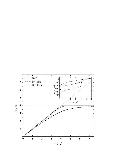
Figure 1: Solutions of the dispersion equations for the second mode, for different magnetic field values (with continuous lines we represent the approximate solution and with discontinuous lines the exact ones). Note that the light cone curve is the straight line $-z_{1}=z_{2}$. The behavior for $(z_{1}+z_{2})/m^{2}$ is drawn in the upper right figure, in a logarithmic scale, to allow depict the three curves.

We conclude that no component of ${\mathbf{\mu}}_{\gamma}$ perpendicular to $\mathbf{B}$ arises in our problem. But the main conclusion according to EliPRD , after explicit calculations, is the photon paramagnetic behavior ${\mathbf{\mu}}_{\gamma}>0$.

3 Photon anomalous magnetic moment in the one loop approximation

We want to give explicit expressions for the photon magnetic moment, starting from the renormalized eigenvalues of the polarization operator in the one-loop approximation, given in shabad2

$$\kappa_{i}=\frac{2\alpha}{\pi}\int_{0}^{\infty}dt\int_{-1}^{1}d\eta e^{-\frac{t}{b}}\left[\frac{\rho_{i}}{\sinh t}e^{\zeta}+\frac{k^{2}\bar{\eta}^{2}}{2t}\right],$$ (13)

$$\zeta(z_{1},z_{2},B) = -\frac{z_{2}}{eB}\frac{\sinh(\eta_{+}t)\sinh(\eta_{-}t)}{\sinh t}-\frac{z_{1}}{eB}\bar{\eta}^{2}t,$$

$$\rho_{1}(z_{1},z_{2}) = -\frac{k^{2}}{2}\frac{\sinh(\eta_{+}t)\cosh(\eta_{+}t)}{\sinh t}\eta_{-},$$

$$\rho_{2}(z_{1},z_{2}) = -\frac{z_{1}}{2}\bar{\eta}^{2}\cosh t-\frac{z_{2}}{2}\frac{\sinh(\eta_{+}t)\cosh(\eta_{+}t)}{\sinh t}\eta_{-},$$

$$\rho_{3}(z_{1},z_{2}) = -\frac{z_{2}}{2}\frac{\sinh(\eta_{+}t)\sinh(\eta_{-}t)}{\sinh^{2}t}$$

$$\hskip 56.9055pt-\frac{z_{1}}{2}\frac{\sinh(\eta_{+}t)\cosh(\eta_{+}t)}{\sinh t}\eta_{-},$$

where we have used the notation $b=\frac{eB}{m^{2}}=\frac{B}{B_{c}}$, $\eta_{\pm}=\frac{1\pm\eta}{2}$, $\bar{\eta}=\sqrt{\eta_{+}\eta_{-}}$.

As we discussed in EliPRD , an explicit expression for a photon magnetic moment $\mu_{\gamma}^{2,3}>0$ in the regions $-z_{1}\leq 4m^{2}$ can be obtained from (13). To that end we differentiate with regard to $B$ the dispersion equation $z_{1}+z_{2}=\kappa_{i}$ and get

$$\frac{\partial z_{1}}{\partial B}=\frac{\partial\kappa_{i}}{\partial B}=\frac{2\alpha}{\pi}\int_{0}^{\infty}dt\int_{-1}^{1}d\eta e^{-\frac{t}{b}}\left[\phi_{i}+\frac{\partial z_{1}}{\partial B}\varphi_{i}\right],$$

$$\phi_{i} = \frac{1}{m^{2}}\left[\frac{\rho_{i}e^{\zeta}}{\sinh t}\left(\frac{t}{b}-\zeta\right)+\frac{k^{2}}{b}\frac{\bar{\eta}^{2}}{2}\right],$$

$$\varphi_{i} = \frac{e^{\zeta}}{\sinh t}\left(\frac{\partial\rho_{i}}{\partial z_{1}}-\frac{\rho_{i}}{eB}\bar{\eta}^{2}t\right)+\frac{\bar{\eta}^{2}}{2t},$$

and, taking in mind that $\frac{\partial z_{1}}{\partial B}=-2\omega\frac{\partial\omega}{\partial B}$ in (3), we obtain a general expression for the photon anomalous magnetic moment

$$\mu_{\gamma}^{i}=-\frac{\partial\omega}{\partial B}=\frac{m^{2}}{2\omega B}\frac{\frac{2\alpha}{\pi}\int_{0}^{\infty}dt\int_{-1}^{1}d\eta e^{-\frac{t}{b}}\phi_{i}}{1-\frac{2\alpha}{\pi}\int_{0}^{\infty}dt\int_{-1}^{1}d\eta e^{-\frac{t}{b}}\varphi_{i}}.$$

It is easy to see that for propagation along $B$ the vacuum behaves as in the limit $B=0$ for all eigenmodes. For that reason, we are mainly interested in studying perpendicular photon propagation case $k_{\parallel}=0$, for which the first mode is non physical. In EliPRD we solved numerically the system of equations (38) and (3), in the interval $0<B<B_{c}$ and confirmed that the paramagnetic behavior is maintained throughout the region of transparency. We stress here that the photon magnetic moment has a maximum on the photon dispersion curve EliPRD near the threshold for pair creation $z_{1}=-4m^{2}+\epsilon$.

3.1 The limit $k^{2}=z_{1}+z_{2}<<eB$

There is wide range of frequencies characterized by the condition $k^{2}=z_{1}+z_{2}<<eB$, which corresponds to small deviations from the light cone $k^{2}=0$. For such frequencies the photon magnetic moment behavior is well described by the following approximate expression (see the Appendix for details)

$$\mu_{\gamma} = -\frac{\partial\omega}{\partial B}$$ (14)

$$= \displaystyle\frac{1}{2\omega}\frac{\frac{\partial\chi_{i}^{(0)}}{\partial B}+\frac{\partial\chi_{i}^{(1)}}{\partial B}k^{2}+\frac{\partial\chi_{i}^{(2)}}{\partial B}k^{4}+\frac{\partial\chi_{i}^{(3)}}{\partial B}k^{6}}{1-\chi_{i}^{(1)}-\frac{\partial\chi_{i}^{(0)}}{\partial z_{1}}-Xk^{2}-Yk^{4}-\frac{\partial\chi_{i}^{(3)}}{\partial z_{1}}k^{6}},$$

$$X = \frac{\partial\chi_{i}^{(1)}}{\partial z_{1}}+2\chi_{i}^{(2)},$$

$$Y = \frac{\partial\chi_{i}^{(2)}}{\partial z_{1}}+3\chi_{i}^{(3)},$$

where the $\chi_{i}^{(l)}$ are functions of $z_{1}$ and $B$

$$\chi_{i}^{(l)} = \frac{2\alpha}{\pi}\int_{0}^{\infty}dt\int_{-1}^{1}d\eta e^{-\frac{t}{b}}\psi_{i}^{l},$$ (15)

$$\psi_{i}^{(0)} = \frac{\rho_{0i}}{\sinh t}e^{\zeta_{0}},$$

$$\psi_{i}^{(1)} = \left[\frac{\rho_{0i}\xi+\theta_{i}}{\sinh t}e^{\zeta_{0}}+\frac{1-\eta^{2}}{8t}\right],$$

$$\psi_{i}^{(l)} = \frac{e^{\zeta_{0}}}{\sinh t}\left[\frac{\rho_{0i}\xi^{l}}{l!}+\frac{\theta_{i}\xi^{l-1}}{(l-1)!}\right],\hskip 28.45274ptl=2,3,...,$$

and $\omega$, $k^{2}$ are given by

$$k^{2} = \frac{\sqrt[3]{R+\sqrt{\frac{Q^{3}}{\left(\chi_{i}^{(3)}\right)^{2}}+R}}+\sqrt[3]{R-\sqrt{\frac{Q^{3}}{\left(\chi_{i}^{(3)}\right)^{2}}+R}}}{\sqrt[3]{\left(\chi_{i}^{(3)}\right)^{2}}}$$ (16)

$$\hskip 159.3356pt-\frac{\chi_{i}^{(2)}}{3\chi_{i}^{(3)}},$$

$$R = -\frac{1}{2}\left[\chi_{i}^{(0)}\chi_{i}^{(3)}-\frac{1}{3}\left(\chi_{i}^{(1)}-1\right)\chi_{i}^{(2)}+\frac{2}{27}\left(\chi_{i}^{(2)}\right)^{2}\right],$$

$$Q = \frac{1}{3}\left[\left(\chi_{i}^{(1)}-1\right)\chi_{i}^{(3)}-\frac{1}{3}\left(\chi_{i}^{(2)}\right)^{2}\right].$$

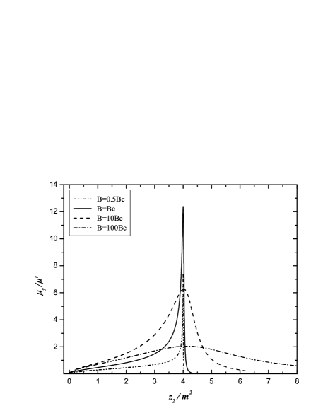
Figure 2: Photon anomalous magnetic moment for the second mode.

We have found a cubic-in-$k^{2}$ approximation for the dispersion curve, which as we see in Fig. 1, is valid in the whole region of transparency for small deviations from the light cone dispersion equation. The approximate curves can be compared to the exact ones, which in both cases were drawn numerically. We conclude from Fig. 2 that in the region of transparency the paramagnetic photon behavior is maintained for supercritical fields: by fixing $z_{2}$, we observe that the quantity $-z_{1}$, and in consequence $\omega$, decreases with increasing $B$.

4 The decrease of frequency with increasing field

In EliPRD we showed that in the region of transparency $\mu_{\gamma}^{i}=-\partial\omega^{i}/\partial B>0$, which means that $\partial\omega^{i}/\partial B<0$. This means that the frequency decreases with increasing field, that is, the incoming photon is red-shifted. (In the case of a gravitational field, for the incoming photon the frequency increases with increasing the modulus of the field gravredshift ). We will give below detailed expressions, especially for the small departure from the light cone case.

It is very important to consider at this point two limits for the dispersion equations: the low frequency quasi-photon limit $\omega\ll 2m$ (small departure from the light cone), and the high frequency quasi-pair limit, which occurs for the second mode when $z_{1}\lesssim-4m^{2}$. In this case $\kappa^{2}$ has a inverse square root divergence, and the solution of the dispersion equation shows a very strong departure from the light cone. In the first case, the expansion of $\kappa^{i}$ in the low frequency, low magnetic field $b=B/B_{c}<1$ limit, and the resulting dispersion equations, was discussed in EliPRD . The dispersion equation, written as $\omega^{2}=|{\bf{k}}^{2}|+\kappa^{(i)}(z_{2},eB)$ is such that $\kappa^{(i)}(z_{2},eB)\ll\omega^{2}$. Thus, as said earlier, the photon self-energy acts as a small perturbation to the light cone equation. The high frequency limit was discussed in shabad2 . In that case, for instance, for the second mode, near the first resonance frequency $z_{1}\lesssim-4m^{2}$, it is $\kappa^{(2)}(z_{2},eB)\gg\omega^{2}$, (in other words, for Landau quantum numbers $n,n^{\prime}=0,1,2,..$ the polarization tensor has an infinite set of branching points at values $z_{1}=(E_{0n}+E_{0n^{\prime}})^{2}$, where $E_{0n}=\sqrt{m^{2}+2eBn}$ and $E_{0n^{\prime}}=\sqrt{m^{2}+2eBn^{\prime}}$). The polarization operator diverges and it is not strictly a “perturbation” but becomes the dominant term. It leads to a quasi-particle which behaves as a massive vector boson, and we name it quasi-pair. Its phase and group velocities are smaller than $c$.

For the quasi-photon limit, by taking the first two terms in the $\kappa^{(i)(0)}$ series expansion in powers of $b^{2}$, and up to fields very close to $B_{c}$ (for instance, $B\sim 0.4B_{c}$), in the series expression for the functions $f^{(2,3)}$, defined in Sec. 2, one can neglect terms from the power $b^{4}$ on. One has $f^{(2,3)}/k_{\perp}^{2}=-\frac{C^{i}\alpha b^{2}}{45\pi}\ll 1$, and as a good approximation the dispersion equations for these modes we have,

$$\omega^{i2}-k^{2}_{\parallel}=k_{\perp}^{2}\left(1-\frac{C^{i}\alpha b^{2}}{45\pi}\right)$$ (17)

where $C^{i}=7,4$ for $i=2,3$. Eq. (17) must be interpreted as the dispersion equation in presence of the magnetic field for an incoming photon which initially, far from the magnetized region, satisfied the usual light cone equation $\omega_{0}^{2}=k^{2}_{\parallel}+k_{\perp}^{2}$. In other words, the dispersion equation before the magnetic field was switched on. The effect of the magnetic field is to decrease the incoming transverse momentum squared by a factor $g(B)^{(i)}=1-f(B)^{(i)}/k_{\perp}^{2}<1$ , to the effective value $k_{eff\perp}^{2}=k_{\perp}^{2}g(B)^{(i)}<k_{\perp}^{2}$ (and in consequence, the initial photon energy decreased from $\omega_{0}\to\omega$, where $\omega=\sqrt{k^{2}_{\parallel}+k_{eff\perp}^{2}}$. Thus, as stated previously, the transverse momentum is not conserved in the magnetic field, and $k_{eff\perp}$ is the effective transverse momentum measured by an observer located in the region where the magnetic field is $\mathbf{B}$. For propagation orthogonal to $\mathbf{B}$, it is $\omega=\omega_{0}\sqrt{g(B)^{(i)}}$, since $\omega_{0}=k_{\perp}$. The non conservation of momentum leads to the decrease of the photon energy, which is red-shifted for incoming photons.

The magnetic field drains (gives) momentum (and energy) to the incoming (outgoing) photon. The case is just the opposite of the gravitational case, in which the gravitational field increases (decreases) the incoming (outgoing) photon momentum (and energy).

Let us devote some space to remind the gravitational field case (we shall use in this paragraph the speed of light as $c$). The last statements can be seen by starting from the Hamilton-Jacobi equation in the massless limit (the action function $S$ becomes the eikonal). Landau . For a photon moving in a centrally symmetric gravitational field the constants of motion are the energy $\omega_{0}$ and angular momentum $L$ with regard to its center. The linear momentum is not a constant of motion. Very far from the massive body, the total energy is $\omega_{0}$, its linear momentum is $k_{0}=\omega_{0}/c$. Near the massive body of mass $M$, for $r>r_{G}$, by calling $e^{\nu}=1-r_{G}/r$, where $r_{G}=2GM/c^{2}$ is the gravitational radius of the body, we can write for a massless particle whose squared effective radial momentum defined by $k_{r}^{2}=e^{\nu}(\partial S/\partial r)^{2}$ as

$$k_{r}^{2}+\frac{L^{2}}{r^{2}}=e^{-\nu}k_{0}^{2},$$ (18)

which expresses the total effective squared momentum as the effective squared energy $\omega_{G}^{2}=e^{-\nu}\omega_{0}^{2}$ divided by $c^{2}$. The observed photon energy (frequency) has been increased from $\omega_{0}$ to $\omega_{G}=e^{-\nu/2}\omega_{0}$. Notice that for $r_{G}\ll r$, one may write, by taking approximately $\omega_{G}\simeq(1+r_{G}/2r)\omega_{0}$,

$$c\sqrt{k_{r}^{2}+(L^{2}/r^{2})}-\frac{r_{G}\omega_{0}}{2r}=\omega_{0}$$ (19)

which expresses in a transparent way the energy conservation, and that the observed (kinetic) energy for the approaching photon is $\omega_{G}>\omega_{0}$ Landau , whereas its interaction energy with the body of mass $M$ is negative. For very large $r$, (19) leads back to $k_{0}c=\omega_{0}$.

4.1 Speed of light orthogonal to $\mathbf{B}$ and vacuum compression

Lorentz transformations in non-parallel directions change the magnetic field to $\mathbf{B}^{\prime}$ and leads to the arising of an electric field $\textbf{E}^{\prime}$, preserving the invariance of ${\cal F}=2B^{2}=2(B^{\prime 2}-E^{\prime 2})$, but leading to inequivalent solutions of the equations of motion. However, they are physically good. Lorentz frames parallel to $\mathbf{B}$ are preferred to preserve the simplicity of the case $\mathbf{B}\neq 0$, $\mathbf{E}=0$. In all of them the photon propagation have equivalent dynamics. It is easy to see that $\partial\omega/\partial k_{\parallel}=1$ in these frames.

As the transverse momentum is not conserved, the speed of light orthogonal to $\mathbf{B}$, if taken as

$$\partial\omega^{i}/\partial k_{\perp}<1$$ (20)

seems to lead to a sub-luminal speed of photons. This interpretation, however, is logically unsatisfactory: one starts from a relativistic invariant theory (Quantum Electrodynamics) and from results obtained perturbatively in the context of this theory in a magnetized medium, concludes that the cornerstone of the relativistic invariance is violated. We maintain the relativistic principle of constancy of the speed of light in vacuum as valid, and claim that (20) expresses the fact that the non-conserved momentum transverse to the field B has an effective value smaller than $k_{\perp}$. In doing that, we state that due to the non-conservation of transverse momentum $k_{\perp}$, both its initial value $k_{\perp}$ and energy $\omega_{0}$ have been decreased to $k_{eff\perp}$, $\omega^{i}$ and the transverse speed of light must be expressed by the equation $\partial\omega^{i}/\partial k_{eff\perp}=1$, in full analogy to the gravitational field case. That is, local observers would find the transverse speed of light as unity. For them, from (17), the light cone equation can be written in coordinate space as

$$\left[\frac{\partial^{2}}{\partial x_{1}^{2i\prime}}+\frac{\partial^{2}}{\partial x_{2}^{2i\prime}}+\frac{\partial^{2}}{\partial x_{3}^{2}}-\frac{\partial^{2}}{\partial x_{0}^{2}}\right]\Psi^{i}=0$$ (21)

where $x_{1,2}^{i\prime}=x_{1,2}^{i}/\sqrt{g(B)^{(i)}}>x_{1,2}^{i}$. This means that the local observer measures, for instance, longer wavelengths, since any rule for measuring lengths if placed in magnetized vacuum, is compressed in the direction orthogonal to $\mathbf{B}$ in the amount $\sqrt{g(B)^{(i)}}$. The longer wavelength is in correspondence to the observed smaller frequencies $\omega^{i}<\omega_{0}$. The vacuum compression is due to the negative pressure effect of magnetized vacuum in the direction perpendicular to the field $\mathbf{B}$ discussed in Elizabeth . Such compression is related to the following facts: the quantity $S_{B}=c\hbar/eB$ can be considered as the quantum of area corresponding to a flux quantum for a field intensity $\mathbf{B}$. Thus, by increasing $B$, $S_{B}$ decreases. As a consequence, the spread of the electron and positron wave functions decreases exponentially with $B$ in the direction orthogonal to the field since they depend on the transverse coordinates as $e^{-\xi^{2}}$ where $\xi^{2}=x_{\perp}^{2}/S_{B}$.

These results mean space-time consequences which bear some analogy to general relativity: we have seen that the vacuum orthogonal to the field behaves as compressed; and also that the red shift means shorter frequencies. But this, in turn, leads to the fact that if time is measured by the wave modes periods $T^{(i)}=2\pi/\omega^{(i)}$, it runs faster for increasing $B$ and do it in a polarization-dependent way and for waves propagating non parallel to $\bf{B}$.

The previous discussion is valid for the low frequency $\omega\ll 2m$, low magnetic field limit, $B\ll B_{c}$, when the spacing between Landau levels is small compared to $2m$. As the field intensity increases the quantity $g(B)$ decreases. The role of the separation between Landau levels of virtual pairs becomes more and more significant as one approaches the first threshold of resonance, which is the quasi-pair region, where $B\lesssim B_{c}$. For frequencies $\omega\simeq 2m$ and $k_{\parallel}<\omega$, the dispersion equation for the second mode may be written shabad2 , since the polarization operator is expressed as a sum over Landau levels $n,n^{\prime}$ of the virtual electron-positron pairs, in terms of the dominant term $n=n^{\prime}=0$, as

$$z_{1}+z_{2}=\frac{2\alpha eBme^{-z_{2}/2eB}}{\sqrt{z_{1}+4m^{2}}}.$$ (22)

This equation is valid in a neighborhood of $z_{1}\lesssim-4m^{2}$. Notice that its limit for $\bf{k}\to 0$ is $\omega\neq 0$. Actually, it describes a massive vector boson particle closely related to the electron-positron pair (see below). This is not in contradiction with the gauge invariance property of the photon self energy. Eq. (22) has solutions found by Shabad shabad2 as those of a cubic equation. One can estimate its behavior very near $z_{1}=-4m^{2}$, by assuming $z_{1}=-4m^{2}+\epsilon$ and $z_{2}=4m^{2}-\epsilon$, the initial energy and transverse momentum where $\epsilon$ is a small quantity. One can obtain the solution approximately as $(z_{1}+4m^{2})^{3/2}=2\alpha eBme^{-z_{2}/2eB}$, from which $z_{1}=-4m^{2}+(2\alpha eBme^{-z_{2}/2eB})^{2/3}$. This means approximately $\omega^{2}=\sqrt{k_{\parallel}^{2}+4m^{2}-(2\alpha eBme^{-2m^{2}/eB})^{2/3}}$. Thus, the transverse momentum of the original photon is trapped by the magnetized medium, the resulting quasi-particle being deviated to move along the field as a vector boson of mass $\omega_{t}=\sqrt{4m^{2}-m^{2}(2\alpha be^{-2/b})^{2/3}}$. Our approach is approximate. A more complete discussion would be made by following the method of shabad2 . This quasi-pair is obviously paramagnetic, as can be checked easily. It differs totally from photons originally propagating parallel to $\mathbf{B}$. For slightly larger energies such that $z_{1}\lesssim-4m^{2}$, and $b$ of order unity, that is $B\sim B_{c}$, they decay in observable electron-positron pairs, and the polarized vacuum becomes absorptive (see shabad2 ). Thus, near the critical field $B_{c}$ our problem bears some analogy to the gravitational singularity effects on light. For light passing near a black hole, if $r\simeq r_{G}$, the light is deviated enough to be absorbed by the black hole. Among other differences in both cases, it must be remarked that the gravitational field in black holes is usually centrally symmetric, whereas our magnetic field is axially symmetric.

5 The red-shift of the paramagnetic photon

For the specific case of the magnetic field produced by a star, we assume that it has axial symmetry and that it decreases with increasing distance along the plane orthogonal to it. In place of assuming an explicit dependence $\mathbf{B}=\mathbf{B}(\textbf{r})$, we assume a partition in concentric shells, in which the magnetic field is considered as constant inside each one. Then $B$ increases to $B+\Delta B$ when passing from a shell to its inner neighbor, and decreases $B-\Delta B$ when passing to the outer one.

From (17), the frequency is red shifted when passing from a region of magnetic field $B$ to another of increased field $B+\Delta B$. In the same limit it is,

$$\Delta\omega^{(2)}=-\frac{14\alpha z_{2}b\Delta b}{45\pi|\textbf{k}|}<0,$$ (23)

and

$$\Delta\omega^{(3)}=-\frac{8\alpha z_{2}b\Delta b}{45\pi|\textbf{k}|}<0.$$ (24)

Here $\Delta b=\Delta B/B_{c}$. Thus, the red shift, consequence of the photon paramagnetism, differs for longitudinal and transverse polarizations.

To give an order of magnitude, for instance, for photons of frequency $10^{20}$ Hz, and magnetic fields of order $10^{12}$ G, $|\Delta\omega|\sim 10^{-6}\omega$.

For the quasi-pair case, from EliPRD , when $z_{1}\to-4m^{2}+\epsilon$ the photon redshift can be written approximately, by calling $P=4m^{2}+z_{1}$. $U=\alpha m^{3}e^{-z_{2}/2eB}$, as

$$\Delta\omega^{(2)}=-\frac{PU}{\omega B_{c}(P^{3/2}+bU)}\left(1+\frac{z_{2}}{2eB}\right)\Delta B<0,$$ (25)

The coefficient of $\Delta B$ at the right, which is minus the photon magnetic moment, has a maximum located on the dispersion curve near the threshold for pair creation $z_{1}=-4m^{2}+\epsilon$. In terms of

$$\omega_{t}=\sqrt{4m^{2}-m^{2}[2\alpha b\exp{(-2/b)}]^{2/3}},$$ (26)

this maximum is

$$\mu_{\gamma}^{(2)}=\frac{e(1+2b)}{3\omega_{t}b}\left[2\alpha b\exp{(-2/b)}\right]^{2/3}$$ (27)

which for $b\sim 1$ is about $13\mu^{\prime}$, where $\mu^{\prime}$ is the anomalous electron magnetic moment.

For supercritical fields $B\to B_{c}/4\alpha$, $\mu_{\gamma}^{(2)}$ (given by the expression (27)) may become arbitrarily large. But this formula is not valid in the mentioned limit $B\to B_{c}/4\alpha$, for which the condition $z_{1}\ll 4m^{2}$ is also satisfied when $z_{2}\approx 4m^{2}$. In that case, according to Shabad3 , the right approximate dispersion equation is

$$z_{1}=-\frac{z_{2}}{1+\frac{\alpha}{3\pi}b},$$ (28)

and, as a consequence, the photon anomalous magnetic moment (for perpendicular photon propagation) looks like

$$\mu_{\gamma}^{(2)}=\frac{\alpha e}{6\pi m^{2}}\frac{\sqrt{z_{2}}}{1+\frac{\alpha}{3\pi}b}.$$ (29)

It is easy to see from (29) that $\mu_{\gamma}^{(2)}$ uniformly tends to zero when the magnetic field grows $b\rightarrow\infty$.

Notice that (23),(24) are the analog of the gravitational red shift gravredshift

$$\Delta\omega_{g}=-\frac{\Delta\phi}{c^{2}}\omega,$$ (30)

where $\Delta\phi=-GM/r_{2}+GM/r_{1}$ and $r_{2}>r_{1}$. However since the gravitational field is negative, $\Delta\phi>0$ corresponds to a decrease in the absolute value of $\phi$, as opposite to $\Delta B>0$. But as pointed out earlier, the magnetic red shift is produced with opposite sign than the gravitational red shift. For $r_{2}\to\infty$ the photon gravitational red shift is $\Delta\omega_{g}=-r_{G}/2r$; this is what is observed for the light coming from a star of mass $M$. For a neutron star of mass $M\sim M_{\bigodot}$, and star radius $r_{1}\sim 10$ Km, $\omega_{g}/\omega\sim 10^{-1}$. The magnetic red shift for the same star, at frequencies of order $\omega=2m$ and field $B\sim B_{c}$ is $\Delta\omega_{B}/\omega=\int_{0}^{B}\mu_{\gamma}^{i}dB/\omega\sim 10^{-5}$. This implies that the magnetic red shift is a small correction to the gravitational red shift up to critical fields.

6 Conclusions

We have shown that the photon magnetic moment ${\mathbf{\mu}}_{\gamma}^{(i)}$ can be understood as as a pseudovector quantity, which is linear in the electromagnetic field tensor ${\cal{F}_{\mu\nu}}$. A cubic in $k^{2}$ approximation for the polarization operator was obtained, from which analytic solutions of the photon dispersion equations and anomalous magnetic moment are easily deduced. These approximate expressions are valid in a very wide range of photon momentum and magnetic fields, whenever the condition $k^{2}/eB\ll 1$ is satisfied. In the whole region of transparency the paramagnetic photon behavior is maintained, even for supercritical fields $B>B_{c}$.

In the region of transparency and for magnetic fields $B\ll B_{c}$ and frequencies $\omega\ll 2m$ photons propagate in magnetized vacuum with energies and transverse momentum decreasing for increasing fields, and vice-versa: it behaves as a tiny dipole moving at the speed of light in magnetized vacuum. For larger magnetic fields $B\simeq B_{c}$ and frequencies $\omega\lesssim 2m$, the resulting quasi–particle behaves as a massive vector boson moving parallel to the field B, its mass being $m_{q}\lesssim 2m$. The last behavior extends to all the region of transparency for supercritical fields $B\gg B_{c}$. It has been discussed the analogy between the photon propagation in a magnetic field and in a gravitational field. Red shift is produced also in the magnetic field case, but with opposite sign than the gravitational one, leading also to space-time deformations.

The presented results, related to the photon propagation in a uniform magnetic field, may be applied to the study of photons in an axially symmetric magnetic field $B=B(x_{\perp})$, by considering concentric shells in which the field is taken as uniform, but varying from shell to shell. This can be made whenever the variation of $B$ over the length $l=\sqrt{\hbar c/eB}$ is negligibly small. We have found a that the photon magnetic moment has a maximum on the dispersion curve, in the region close to the electron-positron pair creation threshold.

The study of photon properties in an external magnetic field Adler -ShabadUsov is very important in the astrophysical context, where high magnetic fields have been estimated to exist GRB -magnAstroph2 ; and can be considered as an important part of a more general problem: the theoretical study of high energy processes of elementary particles in strong external electromagnetic fields. Nowadays, this issue has also attracted the interest of several experimental researchers, due to the development of high power lasers and ion accelerators (see tev ,Muller and references therein).

Appendix A Series expansion of the polarization operator

A.1 $k^{2}=z_{1}+z_{2}<<eB$ limit

The functions $\zeta$ and $\rho_{i}$ ($i=1,2,3$), linear in $z_{1}$ and $z_{2}$, may also be written as

$$\zeta(z_{1},-z_{1}+k^{2},B) = \zeta_{0}(z_{1},B)+k^{2}\xi(B),$$ (31)

$$\rho_{i}(z_{1},-z_{1}+k^{2}) = \rho_{0i}(z_{1})+k^{2}\theta_{i},$$ (32)

where $\zeta_{0}=\zeta(z_{1},-z_{1},B)$, $\xi=\zeta(0,k^{2},B)/k^{2}$ and $\rho_{0i}=\rho_{i}(z_{1},-z_{1})$, $\theta_{i}=\rho_{i}(0,k^{2})/k^{2}$. We can express then (13) as

$$\kappa_{i}=\sum_{l=0}^{\infty}\chi_{i}^{(l)}k^{2l},$$ (33)

$$\chi_{i}^{(l)} = \frac{2\alpha}{\pi}\int_{0}^{\infty}dt\int_{-1}^{1}d\eta e^{-\frac{t}{b}}\psi_{i}^{l},$$ (34)

$$\psi_{i}^{(0)} = \frac{\rho_{0i}}{\sinh t}e^{\zeta_{0}},$$

$$\psi_{i}^{(1)} = \left[\frac{\rho_{0i}\xi+\theta_{i}}{\sinh t}e^{\zeta_{0}}+\frac{1-\eta^{2}}{8t}\right],$$

$$\psi_{i}^{(l)} = \frac{e^{\zeta_{0}}}{\sinh t}\left[\frac{\rho_{0i}\xi^{l}}{l!}+\frac{\theta_{i}\xi^{l-1}}{(l-1)!}\right],\hskip 28.45274ptl=2,3,....$$

We retain only the first four terms in the series expansion (33)

$$\kappa_{i}\approx\chi_{i}^{(0)}+\chi_{i}^{(1)}k^{2}+\chi_{i}^{(2)}k^{4}+\chi_{i}^{(3)}k^{6},$$ (35)

and explicitly solve the resulting approximate dispersion equation, cubic-in-$k^{2}$,

$$0=\chi_{i}^{(0)}+(\chi_{i}^{(1)}-1)k^{2}+\chi_{i}^{(2)}k^{4}+\chi_{i}^{(3)}k^{6}.$$ (36)

The solutions are given by

$$k^{2} = \frac{\sqrt[3]{R+\sqrt{\frac{Q^{3}}{\left(\chi_{i}^{(3)}\right)^{2}}+R}}+\sqrt[3]{R-\sqrt{\frac{Q^{3}}{\left(\chi_{i}^{(3)}\right)^{2}}+R}}}{\sqrt[3]{\left(\chi_{i}^{(3)}\right)^{2}}}$$ (37)

$$\hskip 147.95424pt-\frac{\chi_{i}^{(2)}}{3\chi_{i}^{(3)}},$$

$$R = -\frac{1}{2}\left[\chi_{i}^{(0)}\chi_{i}^{(3)}-\frac{1}{3}\left(\chi_{i}^{(1)}-1\right)\chi_{i}^{(2)}+\frac{2}{27}\left(\chi_{i}^{(2)}\right)^{2}\right],$$

$$Q = \frac{1}{3}\left[\left(\chi_{i}^{(1)}-1\right)\chi_{i}^{(3)}-\frac{1}{3}\left(\chi_{i}^{(2)}\right)^{2}\right].$$

We differentiate with regard to $B$ the dispersion equation (36) and, by using $\frac{\partial z_{1}}{\partial B}=-2\omega\frac{\partial\omega}{\partial B}$ , we obtain finally an expression for the photon anomalous magnetic moment

$$\mu_{\gamma} = -\frac{\partial\omega}{\partial B}$$ (38)

$$= \displaystyle\frac{1}{2\omega}\frac{\frac{\partial\chi_{i}^{(0)}}{\partial B}+\frac{\partial\chi_{i}^{(1)}}{\partial B}k^{2}+\frac{\partial\chi_{i}^{(2)}}{\partial B}k^{4}+\frac{\partial\chi_{i}^{(3)}}{\partial B}k^{6}}{1-\chi_{i}^{(1)}-\frac{\partial\chi_{i}^{(0)}}{\partial z_{1}}-Xk^{2}-Yk^{4}-\frac{\partial\chi_{i}^{(3)}}{\partial z_{1}}k^{6}},$$

$$X = \frac{\partial\chi_{i}^{(1)}}{\partial z_{1}}+2\chi_{i}^{(2)},$$

$$Y = \frac{\partial\chi_{i}^{(2)}}{\partial z_{1}}+3\chi_{i}^{(3)},$$

with $\omega$ and $k^{2}$ given by (37) and

$$\frac{\partial\chi_{i}^{(l)}}{\partial B} = -\frac{2\alpha}{\pi B}\int_{0}^{\infty}dt\int_{-1}^{1}d\eta e^{-\frac{t}{b}}\frac{e^{\zeta_{0}}}{\sinh t}\vartheta_{i}^{(l)}$$ (39)

$$\vartheta_{i}^{(0)} = \rho_{0i}\left[-\frac{t}{b}+\zeta_{0}\right],$$

$$\vartheta_{i}^{(1)} = \left[\left(\rho_{0i}\xi+\theta_{i}\right)\left(-\frac{t}{b}+\zeta_{0}\right)+\rho_{0i}\xi\right]-\frac{\sinh t}{e^{\zeta_{0}}}\frac{1-\eta^{2}}{8b},$$

$$\vartheta_{i}^{(2)} = \left[\left(\frac{\rho_{0i}\xi^{2}}{2}+\theta_{i}\xi\right)\left(-\frac{t}{b}+\zeta_{0}\right)+\rho_{0i}\xi^{2}+\theta_{i}\xi\right],$$

$$\vartheta_{i}^{(3)} = \left[\left(\frac{\rho_{0i}\xi^{3}}{6}+\theta_{i}\frac{\xi^{2}}{2}\right)\left(-\frac{t}{b}+\zeta_{0}\right)+\rho_{0i}\frac{\xi^{3}}{3}+\theta_{i}\xi^{2}\right],$$

$$\frac{\partial\chi_{i}^{(l)}}{\partial z_{1}} = -\frac{2\alpha}{\pi z_{1}}\int_{0}^{\infty}dt\int_{-1}^{1}d\eta e^{-\frac{t}{b}}\upsilon_{i}^{(l)}$$ (40)

$$\upsilon_{i}^{(0)} = \frac{\rho_{0i}}{\sinh t}e^{\zeta_{0}}\left(\zeta_{0}+1\right),$$

$$\upsilon_{i}^{(1)} = \frac{e^{\zeta_{0}}}{\sinh t}\left[\left(\rho_{0i}\xi+\theta_{i}\right)\zeta_{0}+\rho_{0i}\xi\right],$$

$$\upsilon_{i}^{(2)} = \frac{e^{\zeta_{0}}}{\sinh t}\left[\left(\frac{\rho_{0i}\xi^{2}}{2}+\theta_{i}\xi\right)\zeta_{0}+\rho_{0i}\frac{\xi^{2}}{2}\right],$$

$$\upsilon_{i}^{(3)} = \frac{e^{\zeta_{0}}}{\sinh t}\left[\left(\frac{\rho_{0i}\xi^{3}}{6}+\theta_{i}\frac{\xi^{2}}{2}\right)\zeta_{0}+\rho_{0i}\frac{\xi^{3}}{6}\right].$$

References

- (1) H. Pérez Rojas and E. Rodríguez Querts, Phys. Rev. D 79, 093002 (2009)
- (2) A. E. Shabad, Ann. Phys. 90, 166 (1975).
- (3) Ch. Kittel, Introduction to Solid State Physics, John Wileys and Sons, New York (1996).
- (4) S. Villalba, Phys. Rev. D 81, 105019, (2010)
- (5) S. Villalba-Chavez,A.E. Shabad, Phys.Rev. D 86, 105040, (2012)
- (6) H. Pérez Rojas, E. Rodriguez Querts and J. Helayel Netto, Jour. of Mod. Phys. E 20 (2011)
- (7) M.H. Johnson, B.A. Lippmann, Phys. Rev. 76, 828 (1949)
- (8) S. Coleman, Jour. of Math. Physics, 7, (1966), 787.
- (9) E. S. Fradkin, ZhETF, 29, 121, (1955)(JETP, 2,121 (1956))
- (10) W. Pauli, Handbuch der Physik, 24, 1,161 (1933).
- (11) W. Heisenberg and H. Euler, Zeits. fur Phys. 38, 714 (1936)
- (12) H. Pérez Rojas and E. Rodríguez Querts, Int. J. Mod. Phys. A 213761, (2006).
- (13) T.P. Cheng, Relativity, Gravitation and Cosmology, Oxford University Press, New York, (2005).
- (14) L. D. Landau, E. M. Lifshitz, The Classical Theory of Fields, Pergamon Press (1971).
- (15) A. E. Shabad, in Proc. of the Int. Workshop on Strong Magn. Fields and Neutron Stars, Havana 2003. Edited by Univ. de Porto Alegre, Brazil
- (16) S.L. Adler, Annals Phys. 67, 599-647, (1971) 599-647
- (17) V.N. Baier, V.M. Katkov, Phys.Rev. D75, 073009, (2007).
- (18) A. E. Shabad, V.V. Usov, Phys. Rev. D 81, 125008, (2010).
- (19) T. Piran, AIP Conf. Proc. 784 164-174 (2005).
- (20) V.V. Usov, Astrophys.J. 572, L87 (2002).
- (21) M. Ruderman, The Electromagnetic Spectrum of Neutron Stars, NATO ASI Proceedings , Springer, New York, (2004).
- (22) R. C. Duncan and C. Thompson, Astrophys. J. 392, L9 (1992).
- (23) J. Ambjorn, P. Olesen, Nucl. Phys. B 330, 193 (1990).
- (24) A. Di Piazza, C. Muller, K. Z. Hatsagortsyan, C. H. Keitel, Rev. Mod. Phys. 84, 1177 (2012).