This is a preprint. The revised version of this paper is published as
P. Coretto and F. Giordano (2017). “Nonparametric estimation of the dynamic range of music signals”. Australian & New Zealand Journal of Statistics, Vol. 59(4), pp. 389–412 (download link).

NONPARAMETRIC ESTIMATION OF THE
DYNAMIC RANGE OF MUSIC SIGNALS

Abstract. The dynamic range is an important parameter which measures the spread of sound power, and for music signals it is a measure of recording quality. There are various descriptive measures of sound power, none of which has strong statistical foundations. We start from a nonparametric model for sound waves where an additive stochastic term has the role to catch transient energy. This component is recovered by a simple rate-optimal kernel estimator that requires a single data-driven tuning. The distribution of its variance is approximated by a consistent random subsampling method that is able to cope with the massive size of the typical dataset. Based on the latter, we propose a statistic, and an estimation method that is able to represent the dynamic range concept consistently. The behavior of the statistic is assessed based on a large numerical experiment where we simulate dynamic compression on a selection of real music signals. Application of the method to real data also shows how the proposed method can predict subjective experts’ opinions about the hifi quality of a recording.

Keywords: random subsampling, nonparametric regression, music data, dynamic range.

AMS2010: 97M80 (primary); 62M10, 62G08, 62G09, 60G35 (secondary)

1 Introduction

Music signals have a fascinating complex structure with interesting statistical properties. A music signal is the sum of periodic components plus transient components that determine changes from one dynamic level to another. The term “transients” refers to changes in acoustic energy. Transients are of huge interest. For technical reasons most recording and listening medium have to somehow compress acoustic energy variations, and this causes that peaks are strongly reduced with respect to the average level. The latter is also known as “dynamic range compression”. Compression of the dynamic range (DR) increases the perceived loudness. The DR of a signal is the spread of acoustic power. Loss of DR along the recording-to-playback chain translates into a loss of audio fidelity. While DR is a well established technical concept, there is no consensus on how to define it and how to measure it, at least in the field of music signals. DR measurement has become a hot topic in the audio business. In 2008 the release of the album “Death Magnetic” (by Metallica), attracted medias’ attention for its extreme and aggressive loud sounding approach caused by massive DR compression. DR manipulations are not reversible, once applied the original dynamic is lost forever (see Katz, 2007; Vickers, 2010, and references therein). Furthermore, there is now consensus that there is a strong correlation between the DR and the recording quality perceived by the listener. Practitioners in the audio industry use to measure the DR based on various descriptive statistics for which little is known in terms of their statistical properties (Boley et al., 2010; Ballou, 2005).

The aim of this paper is twofold: (i) define a DR statistic that is able to characterize the dynamic of a music signal, and to detect DR compression effectively, (ii) build a procedure to estimate DR with proven statistical properties. In signal processing a “dynamic compressor” is a device that reduces the peakness of the sound energy. The idea here is that dynamic structure of a music signal is characterized by the energy produced by transient dynamic, so that the DR is measured by looking at the distribution of transient power. We propose a nonparametric model composed by two elements: (i) a smooth regression function mainly accounting for long term harmonic components; (ii) a stochastic component representing transients. In this framework transient power is given by the variance of the stochastic component. By consistently estimating the distribution of the variance of the stochastic component, we obtain the distribution of its power which, in turn, is the basis for constructing our DR statistic. The DR, as well as other background concepts are given in Sections 2 and 3.

This paper gives four contributions. The idea of decomposing the music signal into a deterministic function of time plus a stochastic component is due to the work of Serra and Smith (1990). However, it is usually assumed that stochastic term of this decomposition is white noise. While this is appropriate in some situations, in general the white noise assumption is too restrictive. The first novelty in this paper is that we propose a decomposition where the stochastic term is an $\alpha$-mixing process, and this assumption allows to accommodate transient structures beyond those allowed by linear processes. The stochastic component is obtained by filtering out the smooth component of the signal, and this is approximated with a simple kernel estimator inspired to Altman (1990). The second contribution of this work is that we develop upon Altman’s seminal paper obtaining a rate optimal kernel estimator without assuming linearity and knowledge of the correlation structure of the stochastic term. An important advantage of the proposed smoothing is that only one data-driven tuning is needed (see Assumption A4 and Proposition 1), while existing methods require two tunings to be fixed by the user (e.g. Hall et al., 1995). Approximation of the distribution of the variance of the stochastic component of the signal is done by a subsampling scheme inspired to that developed by Politis and Romano (1994) and Politis et al. (2001). However, the standard subsampling requires to compute the variance of the stochastic component on the entire sample, which in turn means that we need to compute the kernel estimate of the smooth component over the entire sample. The latter is unfeasible given the astronomically large nature of the typical sample size. Hence, a third contribution of the paper is that we propose a consistent random subsampling scheme that does only require computations at subsample level. The smoothing and the subsampling are discussed in Section 4. A further contribution of the paper is that we propose a DR statistic based on the quantiles of the variance distribution of the stochastic component. The smoothing–subsampling previously described is used to obtain estimates of such a statistic. The performance of the DR statistic is assessed in a simulation study where we use real data to produce simulated levels of compression. Various combinations of compression parameters are considered. We show that the proposed method is quite accurate in capturing the DR concept. DR is considered as a measure of hifi quality, and based on a real dataset we show how the estimated DR measure emulates comparative subjective judgements about hifi quality given by experts. All this is treated in Sections 6 and 7. Conclusions and final remarks are given in Section 8. All proofs of statements are given in the final Appendix.

2 Background concepts: sound waves, power and dynamic

Let $x(t)$ be a continuous time waveform taking values on the time interval $T_{1}\leq t\leq T_{2},$ such that $\int_{T_{1}}^{T_{2}}x(t)dt=0$. Its power is given by

$$P^{RMS}=C\sqrt{\frac{1}{T_{2}-T_{1}}\int_{T_{1}}^{T_{2}}x(t)^{2}dt}$$ (1)

where $C$ is an appropriate scaling constant that depends on the measurement unit. (1) defines the so-called root mean square (RMS) power. It tells us that the power expressed by a waveform is determined by the average magnitude of the wave swings around its average level. In other words the equation (1) reminds us of the concept of standard deviation. A sound wave $x(t)$ can be recorded and stored by means of analog and/or digital processes. In the digital world $x(t)$ is represented numerically by sampling and quantizing the analog version of $x(t)$. The sampling scheme underlying the so-called Compact Disc Digital Audio, is called Pulse Code Modulation (PCM). In PCM sampling a voltage signal $x(t)$ is sampled as a sequence of integer values proportional to the level of $x(t)$ at equally spaced times $t_{0},t_{1},\ldots$ . The CDDA is based on PCM with sampling frequency equal to 44.1KHz, and 16bits precision. The quantization process introduces rounding errors also known as quantization noise. Based on the PCM samples $\{x_{0},x_{1},\ldots x_{T}\}$, and under strong conditions on the structure of the underlying $x(t)$, the RMS power can be approximated by

$$P^{RMS}_{T}=\sqrt{\frac{1}{T+1}\sum_{t=0}^{T}x_{t}^{2}}.$$ (2)

The latter is equal to sampling variance, because this signals have zero mean. Power encoded in a PCM stream is expressed as full-scale decibels:

$$\text{dBFS}=20\log_{10}\frac{P^{RMS}_{T}}{P_{0}},$$ (3)

where $P_{0}$ is the RMS power of a reference wave. Usually $P_{0}=1/\sqrt{2}$, that is, the RMS power of a pure sine-wave, or $P_{0}=1$ that is, the RMS power of pure square-wave. For simplicity we set $P_{0}=1$ in this paper. dBFS is commonly considered as DR measure because it measures the spread between sound power and power of a reference signal.

For most real-world signal power changes strongly over time. In Figure 1 we report a piece of sound extracted from the left channel of the song “In the Flesh?” by Pink Floyd. The song starts with a soft sweet lullaby corresponding to Block 1 magnified in the bottom plot. However, at circa 20.39s the band abruptly starts a sequence of blasting riffs. This teaches us that: (i) sound power of music signals can change tremendously over time; (ii) the power depends on $T$, that is the time horizon. In the audio engineering community the practical approach is to time-window the signal and compute average power across windows, then several forms of DR statistics are computed (see Ballou, 2005) based on dBFS. In practice one chooses a $T$, then splits the PCM sequence into blocks of $T$ samples allowing a certain number $n_{o}$ of overlapping samples between blocks, let $\overline{P^{RMS}}_{T}$ be the average of $P_{T}^{RMS}$ values computed on each block, finally a simple DR measure, that we call “sequential DR”, is computed as

$$\text{DRs}=-20\log_{10}\frac{\overline{P^{RMS}}_{T}}{x_{\text{peak}}},$$ (4)

where $x_{\text{peak}}$ is the peak sample. The role of $x_{\text{peak}}$ is to scale the DR measure so that it does not depend on the quantization range. DRs=10 means that on average the RMS power is 10dBFS below the maximum signal amplitude. Notice that 3dBFS increment translates into twice the power. DRs numbers are easily interpretable, however, the statistical foundation is weak. Since the blocks are sequential, $T$ and $n_{o}$ determine the blocks uniquely regardless the structure of the signal at hand. The second issue is whether the average $\overline{P^{RMS}}_{T}$ is a good summary of the power distribution in order to express the DR concept. Certainly the descriptive nature of the DRs statistic, and the lack of a stochastic framework, does not allow to make inference and judge numbers consistently.

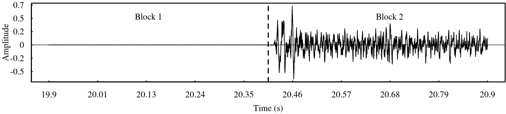
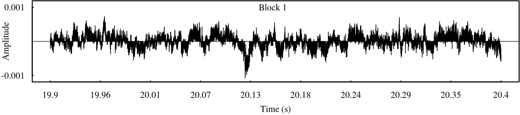
Figure 1: Waveform extracted from the left channel of the song “In the Flesh?” from “The Wall” album by Pink Floyd (Mobile Fidelity Sound Lab remaster, catalog no. UDCD 2-537). Top plot captures 980ms of music centered at time 20.39524s (vertical dashed line). Bottom plot magnifies Block 1.

3 Statistical properties of sound waves and modelling

The German theoretical physicist Herman Von Helmholtz (1885) discovered that within small time intervals sound signals produced by instruments are periodic and hence representable as sums of periodic functions of time also known as “harmonic components”. The latter implies a discrete power spectrum. Risset and Mathews (1969) discovered that the intensity of the harmonic components varied strongly over time even for short time lengths. Serra and Smith (1990) proposed to model sounds from single instruments by a sum of sinusoids plus a white noise process. While the latter can model simple signals, e.g. a flute playing a single tune, in general such a model is too simple to represent more complex sounds.

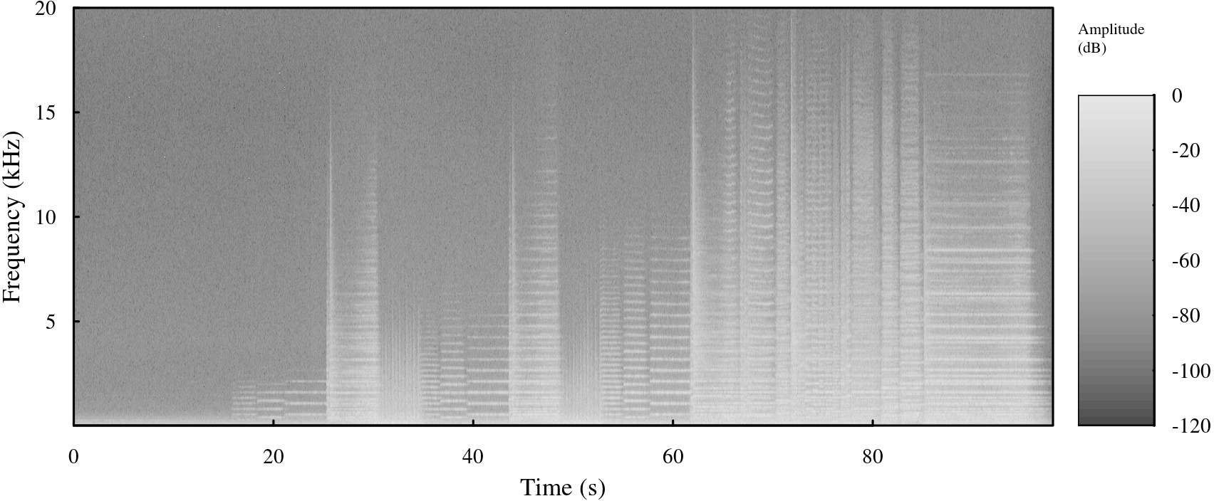
Figure 2: Spectrogram of the right channel of the opening fanfare of “Also Sprach Zarathustra” (Op. 30) by Richard Strauss, performed by Vienna Philharmonic Orchestra conducted by Herbert von Karajan (Decca, 1959). The power spectra values are expressed in dBFS scale and coded as colors ranging from black (low energy) to white (high energy).

Figure 2 reports the spectrogram of a famous fanfare expressed in dBFS. This is a particularly dynamic piece of sound. The orchestra plays a soft opening followed by a series of transients at full blast with varying decay-time. There are several changes in the spectral distribution. At particular time points there are peaks localized in several frequency bands, but there is a continuum of energy spread between peaks. This shows how major variations are characterized by a strong continuous component in the spectrum that is also time-varying. In their pioneering works Voss and Clarke (1975); Voss (1978) found evidence that, at least for some musical instruments, once the recorded signal is passed trough band-pass filter with cutoffs set at 100Hz and 10KHz, the signal within the bandpass has a spectrum that resembles $1/f$–noise or similar fractal processes. But the empirical evidence is based on spectral methods acting as if the processes involved were stationary, whereas this is often not true. Moreover, while most acoustic instruments produce most of their energy between 100Hz and 10KHz, this is not true if one considers complex ensembles. It is well known that for group of instruments playing together, on average 50% of the energy is produced in the range [20Hz, 300Hz]. Whether or not the $1/f$–noise hypothesis is true is yet to be demonstrated, in this paper we give examples that show that the $1/f$–noise hypothesis does not generally hold.

These observations are essential to motivate the following model for the PCM samples. Let $\{Y_{t}\}_{t\in\mathbb{Z}}$ be a sequence such that

$$Y_{t}=s(t)+\varepsilon_{t},$$ (5)

under the following assumptions:

A1.

The function $s(t)$ has a continuous second derivative.

A2.

$\{\varepsilon_{t}\}_{t\in\mathbb{Z}}$ is a strictly stationary and $\alpha$-mixing process with mixing coefficients $\alpha(k)$, $\operatorname{E}[\varepsilon_{t}]=0$, $\operatorname{E}\left|\varepsilon_{t}^{2}\right|^{2+\delta}<+\infty$, and $\sum_{k=1}^{+\infty}\alpha^{\delta/(2+\delta)}(k)<\infty$ for some $\delta>0$.

(5) is by no means interpretable as a Tukey-kind signal plus noise decomposition. The observable (recorded) sound wave $Y_{t}$ deviates from $s(t)$ because of several factors: (i) transient changes in acoustic energy; (ii) several sources of noise injected in the recording path; (iii) non-harmonic components. We call the process $\{\varepsilon_{t}\}_{t\in\mathbb{Z}}$ the “stochastic sound wave” (SSW). The main difference with Serra and Smith (1990) is that in their work $\varepsilon_{t}$ is a white noise, and $s(t)$ is a sum of sinusoids. Serra and Smith (1990) are mainly interested in the spectral structure, hence they use $s(t)$ to study the discrete part of the spectrum. Moreover they are interested in simple sounds from single instruments, hence they simply assume that $\varepsilon_{t}$ is a white noise. Their assumptions are reasonable for simple sounds, but in general do not hold for complex sounds from an ensemble of instruments.

A1 imposes a certain degree of smoothness for $s(\cdot)$. This is because we want that the stochastic term absorbs transients while $s(\cdot)$ mainly models long-term periodic (harmonic) components. The $\alpha$-mixing assumption allows to manage non linearity, departure from Gaussianity, and a certain slowness in the decay of the dependence structure of the SSW. Certainly the $\alpha$-mixing assumption A2 would not be consistent with the long-memory nature of $1/f$–noise. However, the $1/f$–noise features disappear once the long term harmonic components are caught by $s(\cdot)$ (see discussion on the example of Figure 3). Whereas A2 allows for various stochastic structures, the restrictions on the moments and mixing coefficients are needed for technical reasons. Nevertheless, the existence of the fourth moment is not that strong in practice, because this would imply that the SSW has finite power variations, which is something that has to hold otherwise it would be impossible to record it.

4 Estimation

The DR statistic proposed in this paper is estimated based on the following subsampling algorithm.

input : PCM data, $b\in N,K\in N$

output : DR statistic

Draw a random sample $\left\{I_{1},I_{2},\ldots,I_{K}\right\}$ from the set $\left\{1,2,\ldots,n-b+1\right\};$

for $i=1,2,\ldots,K$ do

       optimally estimate $s(\cdot)$ on the subsample $Y^{\text{sub}}_{i}=\left\{y_{I_{i}},y_{I_{i}+1},\ldots,y_{I_{i}+b-1}\right\},$

       compute the sampling variance of $\hat{\varepsilon}$ over $Y^{\text{sub}}_{i}$

end for

Construct the empirical distribution of the variances of $\hat{\varepsilon}$.

Compute the DR statistic based on empirical distribution of the variances of $\hat{\varepsilon}.$

Algorithm 1 blockwise smoothing

In analogy with equation (2), the RMS power of the SSW is given by the sampling standard deviation of $\{\varepsilon_{t}\}_{t\in\mathbb{Z}}$. The main goal is to obtain an estimate of the distribution of the variance of $\{\varepsilon_{t}\}_{t\in\mathbb{Z}}$. Application of existing methods would require nonparametric estimation of $s(\cdot)$ on the entire sample. However, the sample size is typically of the order of millions of observations. Moreover, since the smooth component is time-varying, one would estimate $s(\cdot)$ by using kernel methods with local window. It is clear that all this is computationally unfeasible. Compared with the standard subsampling, the “blockwise smoothing” Algorithm gives clear advantages: (i) randomization reduces the otherwise impossible large number of subsamples to be explored; (ii) none of the computations is performed on the entire sample. In particular estimation of $s(\cdot)$ is performed subsample-wise as in Proposition 2 and Corollary 1; (iii) estimation of $s(\cdot)$ on smaller blocks of observations allows to adopt a global, rather than a local, bandwidth approach. Points (ii) and (iii) are crucial for the feasibility of the computing load. The smoothing and the random subsampling part of the procedure are disentangled in the next two Sections.

4.1 Smoothing

This section treats the smoothing with respect to the entire sample. The theory developed into this section is functional to the development of the local estimation of $s(\cdot)$ at subsample level. The latter will be treated in Section 4.2. First notice that without loss of generality we can always rescale $t$ onto $(0,1)$ with equally spaced values. Therefore, model (5) can be written as

$$Y_{i}=s(i/n)+\varepsilon_{i},\qquad i=1,\ldots,n.$$ (6)

Estimation of $s(t)$, $t\in(0,1)$, is performed based on the classical Priestley-Chao kernel estimator (Priestley and Chao, 1972)

$$\hat{s}(t)=\frac{1}{nh}\sum_{i=1}^{n}\mathcal{K}\left(\frac{t-i/n}{h}\right)y_{i},$$ (7)

under the assumption

A3.

$\mathcal{K}(\cdot)$ is a density function symmetric about zero with compact support. Moreover, $\mathcal{K}(\cdot)$ is Lipschitz continuous of some order. The bandwidth $h\in H=[c_{1}n^{-1/5};c_{2}n^{-1/5}]$, where $c_{1}$ and $c_{2}$ are two positive constants such that $c_{1}$ is arbitrarily small while $c_{2}$ is arbitrarily large.

Without loss of generality, we will use the Epanechnikov kernel for its well known efficiency properties, but any other kernel function fulfilling A3 is welcome. Altman (1990) studied the kernel regression problem when the error term additive to the regression function exhibits serial correlation. Furthermore in the setup considered by Altman (1990) the error term is a linear process. The paper showed that when the stochastic term exhibits serial correlation, standard bandwidth optimality theory no longer applies. The author proposed an optimal bandwidth estimation which is based on a correction factor that assumes that the autocorrelation function is known. Therefore Altman’s theory does not apply here for two reasons: (i) in this paper the $\left\{\varepsilon_{t}\right\}_{t\in\mathbb{Z}}$ is not restricted to the class of linear processes; (ii) we do not assume that serial correlations are known. Let $\hat{\varepsilon}_{i}=y_{i}-\hat{s}(i/n)$, and let us define the cross-validation function

$$\text{CV}(h)=\left[1-\frac{1}{nh}\sum_{j=-M}^{M}\mathcal{K}\left(\frac{j}{nh}\right)\hat{\rho}(j)\right]^{-2}\frac{1}{n}\sum_{i=1}^{n}\hat{\varepsilon}_{i}^{2};$$ (8)

where the first term is the correction factor à la Altman with the difference that it depends on the estimated autocorrelations of $\{\varepsilon_{t}\}_{t\in\mathbb{Z}}$ up to $M$th order. We show that the modification does not affect consistency at the optimal rate. The number of lags into the correction factor depends both on $n$ and $h$. Intuitively consistency of the bandwidth selector can only be achieved if $M$ increases at a rate smaller than $nh$, and in fact we will need the following technical requirement:

A4.

Whenever $n\to\infty$; then $M\to\infty$ and $M=O(\sqrt{nh})$.

The previous condition makes clear the relative order of the two smoothing parameters $M$ and $h$. The bandwidth is estimated by minimizing the cross-validation function, that is

$$\hat{h}={\text{argmin}}_{h\in H}\;\text{CV}(h).$$

Since $t$ is deterministic and equally spaced in $(0,1)$ and, using the approach as in Altman (1990), we can write the Mean Square Error (MSE) of $\hat{s}(t)$ as

$$\mbox{MSE}(h;\hat{s}(t))=\frac{B_{\mathcal{K}}^{2}}{4}h^{4}[s^{\prime\prime}(t)]^{2}+\frac{V_{\mathcal{K}}}{nh}\sigma_{\varepsilon}^{2}(1+2S_{\rho}),$$

where $s^{\prime\prime}(\cdot)$ is the second derivative of $s(\cdot)$, $\sigma_{\varepsilon}^{2}=E(\varepsilon_{t}^{2})$, $S_{\rho}=\sum_{j=1}^{\infty}\rho(j)$, $B_{\mathcal{K}}=\int u^{2}\mathcal{K}(u)du$ and $V_{\mathcal{K}}=\int\mathcal{K}^{2}(u)du$. Let $\text{MISE}(h;\hat{s})$ be the Mean Integrated Square Error of $\hat{s}(\cdot)$, that is

$$\text{MISE}(h;\hat{s})=\int_{0}^{1}\mbox{MSE}(h;\hat{s}(t))dt=\frac{B_{\mathcal{K}}^{2}}{4}h^{4}\int_{0}^{1}[s^{\prime\prime}(t)]^{2}dt+\frac{V_{\mathcal{K}}}{nh}\sigma_{\varepsilon}^{2}(1+2S_{\rho})$$

and let $h^{\star}$ be the global minimizer of $\text{MISE}(h;\hat{s})$.

Proposition 1.

Assume A1, A2, A3 and A4. $\hat{h}/{h^{\star}}\stackrel{{\scriptstyle\text{p}}}{{\longrightarrow}}1$ as $n\to\infty$.

Proof of Proposition 1 is given in the Appendix. It shows that $\hat{h}$ achieves the optimal global bandwidth. The previous result improves the existing literature in several aspects. Previous works on kernel regression with correlated errors all requires stronger assumptions on $\{\varepsilon_{t}\}_{t\in\mathbb{Z}}$, e.g. linearity, Gaussianity, existence of high order moments and some stringent technical conditions (see Altman, 1990, 1993; Hart, 1991; Xia and Li, 2002; Francisco-Fernández et al., 2004). None of the contributions in the existing literature treats the choice of the smoothing parameters in the cross-validation function, that is $M$. Francisco-Fernández et al. (2004) mentions its crucial importance, but no clear indication on how to set it is given. A4 improves upon this giving a clear indication of how this tuning has to be automatically fixed in order to achieve optimality. In fact, Proposition 1 suggests to take $M=\lfloor\sqrt{nh}\rfloor$. Therefore the smoothing step is completely data-driven. Notice that alternatively standard cross-validation would require to fix two tuning parameters (see Theorem 2.3 in Hall et al., 1995).

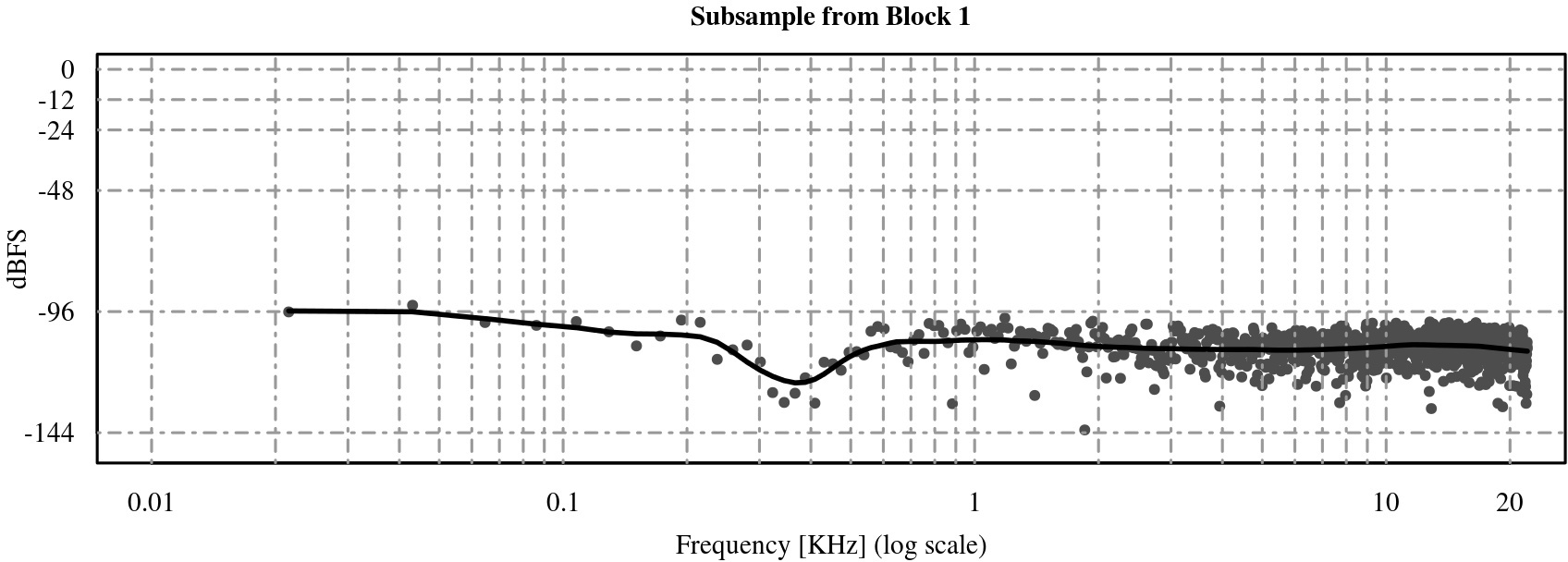
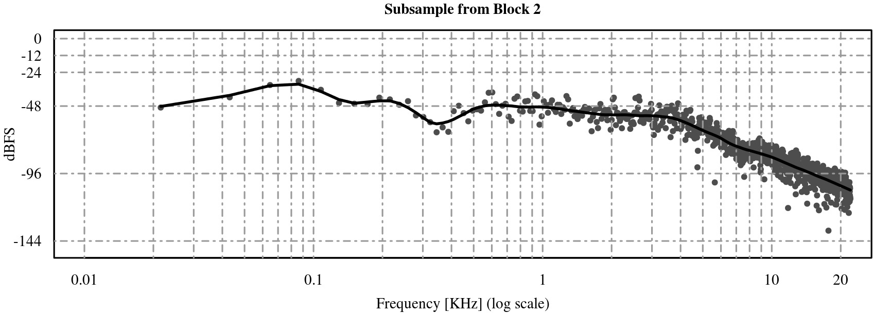
Figure 3: Points represent windowed periodogram power spectral density estimates of the SSW obtained in two subsamples of size 50ms extracted from the wave reported in Figure 1. The solid line has been obtained by kernel smoothing. The top plot refers to a subsample randomly chosen within “Block 1”, while the bottom plot refers to a subsample randomly chosen within “Block 2”.

Figure 4: Estimated signal and squared residuals for a subsamples of 50ms randomly extracted from the second half of the wave reported in Figure 1. The estimated optimal bandwidth is $\hat{h}=0.01521$.

In order to see how the behavior of $\{\varepsilon_{t}\}_{t\in\mathbb{Z}}$ is time-varying, see Figure 3. The SSW has been estimated based on (7) and (8) on subsamples of length equal to 50ms. The first subsample has been randomly chosen within Block 1 of Figure 1, while the second has been randomly chosen within Block 2. Discrete-time Fourier transform measurements have been windowed using Hanning window. Points in the plots correspond to spectral estimates at FFT frequencies scaled to dBFS (log-scale). It can be seen that the two spectrum show dramatic differences. In the first one the energy spread by the SSW is modest and near the shape and level of uncorrelated quantization noise. On the other hand, the bottom spectrum shows a pattern that suggests that correlations vanish at slow rate which is consistent with A2. The steep linear shape of on log-log coordinates above 3KHz reminds us approximately the shape of the $1/f$–noise spectrum, however below 3KHz the almost flat behavior suggests a strong departure from the $1/f$–noise hypothesis. All this confirms the idea that there are music sequences where the SSW in (5) cannot be seen as the usual “error term”. Tests proposed in Berg et al. (2012) also lead to rejection of the linear hypothesis for the SSW. In the end, it is remarkable that these extremely diverse stochastic structures coexist within just one second of music. In Figure 4 we show the estimated $\hat{s}(\cdot)$ against observed data (top panel), and the corresponding $\hat{\varepsilon}_{t}^{2}$ for a 50ms subsample taken from the same song. The large spikes in the bottom panel correspond to situations where the amplitude variations increase unexpectedly so that they are caught by the stochastic component of the model.

4.2 Random Subsampling

Equation (2) only takes into account sum of squares, this is because theoretically PCM are always scaled to have zero mean. Notice that, even though we assume that $\{\varepsilon_{t}\}_{t\in\mathbb{Z}}$ has zero expectation, we define RMS based on variances taking into account the fact that quantization could introduce an average offset in the PCM samples. Let us introduce the following quantities:

$$V_{n}=\frac{1}{n-1}\sum_{i=1}^{n}\left(\varepsilon_{i}-\bar{\varepsilon}\right)^{2},\qquad\text{with}\quad\bar{\varepsilon}=\frac{1}{n}\sum_{i=1}^{n}\varepsilon_{i}.$$ (9)

The distribution of the RMS power of the SSW is given by the distribution of $\sqrt{V_{n}}$. By A2 it can be shown that $\sqrt{n}(V_{n}-\sigma^{2}_{\varepsilon})\stackrel{{\scriptstyle\text{d}}}{{\longrightarrow}}\text{Normal}(0,V),$ where $\sigma^{2}_{\varepsilon}=\operatorname{E}[\varepsilon_{t}^{2}]$ and $V=\lim_{n\rightarrow\infty}n\operatorname{Var}[V_{n}]$. From now onward, $G(\cdot)$ will denote the distribution function of a $\text{Normal}(0,V)$.

Although the sequence $\left\{\varepsilon_{i}\right\}$ is not observable, one can approximate its power distribution based on $\hat{\varepsilon}_{i}=y_{i}-\hat{s}(i/n)$. Replacing $\varepsilon_{i}$ with $\hat{\varepsilon}_{i}$ in (9) we obtain:

$$\hat{V}_{n}=\frac{1}{n-1}\sum_{i=1}^{n}\left(\hat{\varepsilon}_{i}-\bar{\hat{\varepsilon}}\right)^{2},\qquad\text{with}\quad\bar{\hat{\varepsilon}}=\frac{1}{n}\sum_{i=1}^{n}\hat{\varepsilon}_{i}.$$

The distribution of $\hat{V}_{n}$ can now be used to approximate the distribution of $V_{n}$. One way to do this is to implement a subsampling scheme à la Politis et al. (2001). That is, for all blocks of observations of length $b$ (subsample size) one compute $\hat{V}_{n}$, in this case there would be $n-b+1$ subsamples to explore. Then one hopes that the empirical distribution of the $n-b+1$ subsample estimates of $\hat{V}_{n}$ agrees with the distribution of $V_{n}$ when both $n$ and $b$ grow large enough at a certain relative speed. This is essentially the subsampling scheme proposed by Politis et al. (2001) and Politis and Romano (2010), but it is of limited practical use here because the scale of $n$ is usually in millions, and the computation of $\hat{s}(\cdot)$ on the entire sample would require a huge computational effort that is of order $O(n^{2})$. This is because the Kernel estimation procedure requires a number o iterations of order $O(n)$ for each point of the support. On a modern computer an highly optimized software programmed in C language takes about 17 hours to compute $\hat{s}(\cdot)$ on a 3min song ($n=15,876,000$ samples), and about 38 hours for a 4.5min song ($n=23,814,000$). This figures are for a fixed global $h$. If we perform cross-validation on a grid with 25 points (a reasonable choice), the estimate becomes 17 days for a 3min song, and almost 40 days for a 4.5min song. And then one needs to add the computing time needed for the subsampling steps which will depend on $b$ and $K$. The blockwise smoothing algorithm solves the problem by introducing a variant to the classical subsampling scheme previously described. Namely instead of estimating $s(\cdot)$ on the entire series, we estimate it on each subsample separately, then we use the average estimated error computed block-wise instead of $\bar{\hat{\varepsilon}}$ computed on the whole sample. Moreover a blockwise kernel estimate of $s(\cdot)$ allows to work with the simpler global bandwidth instead of the more complex local bandwidth without loosing too much in the smoothing step. The blockwise smoothing algorithm proposed in this paper (with the default choice of $b$ and $K$ discussed afterwards) computes the proposed DR statistic in about 30s on the same computer for a 3min song, this saves us 17 days of computing.

Let $\hat{s}_{b}(\cdot)$ be the estimator of $s(\cdot)$ on a subsample of length $b$, that is

$$\hat{s}_{b}(t)=\frac{1}{bh}\sum_{i=1}^{b}\mathcal{K}\left(\frac{t-i/b}{h}\right)y_{i}.$$ (10)

At a given time point $t$ we consider a block of observations of length $b$ and we consider the following statistics

$$V_{n,b,t}=\frac{1}{b-1}\sum_{i=t}^{t+b-1}(\varepsilon_{i}-\bar{\varepsilon}_{b,t})^{2},\qquad\text{and}\qquad\hat{V}_{n,b,t}=\frac{1}{b-1}\sum_{i=t}^{t+b-1}(\hat{\varepsilon}_{i}-\bar{\hat{\varepsilon}}_{b,t})^{2},$$

with $\bar{{\varepsilon}}_{b,t}=b^{-1}\sum_{i=t}^{t+b-1}{\varepsilon}_{i}$ and $\bar{\hat{\varepsilon}}_{b,t}=b^{-1}\sum_{i=t}^{t+b-1}\hat{\varepsilon}_{i}$. Note that in $\hat{V}_{n,b,t}$ we can consider either $\hat{\varepsilon}_{i}=y_{i}-\hat{s}(i/n)$ or $\hat{\varepsilon}_{i}=y_{i}-\hat{s}_{b}((i-t+1)/b)$, $i=t,\ldots,t+b-1$. Of course, the bandwidth, $h$, depends on $n$ or $b$. We do not report this symbol because it will be clear from the context. The empirical distribution functions of $V_{n,b,t}$ and $\hat{V}_{n,b,t}$ will be computed as

$$G_{n,b}(x) = \frac{1}{n-b+1}\sum_{t=1}^{n-b+1}\text{\bf\large 1}\left\{\sqrt{b}\left(V_{n,b,t}-V_{n}\right)\leq x\right\},$$

$$\hat{G}_{n,b}(x) = \frac{1}{n-b+1}\sum_{t=1}^{n-b+1}\text{\bf\large 1}\left\{\sqrt{b}(\hat{V}_{n,b,t}-V_{n})\leq x\right\};$$

where $\text{\bf\large 1}\left\{A\right\}$ denotes the usual indicator function of the set $A$. Furthermore, the quantiles of the subsampling distribution also converges to the quantities of interest, that is those of $V_{n}$. This is a consequence of the fact that $\sqrt{n}V_{n}$ converges weakly to a Normal distribution, let it be $F$. Let define the empirical distributions:

$$F_{n,b}(x) = \frac{1}{n-b+1}\sum_{t=1}^{n-b+1}\text{\bf\large 1}\left\{\sqrt{b}V_{n,b,t}\leq x\right\},$$

$$\hat{F}_{n,b}(x) = \frac{1}{n-b+1}\sum_{t=1}^{n-b+1}\text{\bf\large 1}\left\{\sqrt{b}\hat{V}_{n,b,t}\leq x\right\}.$$

For $\gamma\in(0,1)$ the quantities $q(\gamma)$, $q_{n,b}(\gamma)$ and $\hat{q}_{n,b}(\gamma)$ denote respectively the $\gamma$-quantiles with respect to the distributions $F$, $F_{n,b}$ and $\hat{F}_{n,b}$. We adopt the usual definition that $q(\gamma)=\inf\left\{x:F(x)\geq\gamma\right\}$. However exploring all subsamples makes the procedure still computationally heavy. A second variant is to reduce the number of subsamples by introducing a random block selection. Let $I_{i}$, $i=1,\ldots K$ be random variables indicating the initial point of every block of length $b$. We draw the sequence $\left\{I_{i}\right\}_{i=1}^{K}$, with or without replacement, from the set $I=\{1,2,\ldots,n-b+1\}$. The empirical distribution function of the subsampling variances of $\varepsilon_{t}$ over the random blocks will be:

$$\tilde{G}_{n,b}(x)=\frac{1}{K}\sum_{i=1}^{K}\text{\bf\large 1}\left\{\sqrt{b}\left(\hat{V}_{n,b,I_{i}}-V_{n}\right)\leq x\right\},$$

and the next results states the consistency of $\tilde{G}$ in approximating $G$.

Proposition 2.

Assume A1, A2, A3 and A4. Let $\hat{s}_{b}(t)$ be the estimator of $s(t)$ on a subsample of length $b$. If $K\rightarrow\infty$, $b/n\rightarrow 0$, $b\rightarrow\infty$ then $\sup_{x}\left|\tilde{G}_{n,b}(x)-G(x)\right|\stackrel{{\scriptstyle\text{p}}}{{\longrightarrow}}0$ when $n\rightarrow\infty$.

We can also establish consistency for the quantiles based on $\left\{\hat{V}_{n,b,I_{i}}\right\}_{i=1}^{K}$. Let define the distribution function

$$\tilde{F}_{n,b}(x)=\frac{1}{K}\sum_{t=1}^{K}\text{\bf\large 1}\left\{\sqrt{b}\hat{V}_{n,b,I_{t}}\leq x\right\},$$

and let $\tilde{q}_{n,b}(\gamma)$ be the $\gamma$-quantile with respect to $\tilde{F}$.

Corollary 1.

Assume A1, A2, A3 and A4. Let $\hat{s}_{b}(t)$ be the estimator of $s(t)$ on a subsample of length $b$. If $K\rightarrow\infty$, $b/n\rightarrow 0$, $b\rightarrow\infty$ then $\tilde{q}_{n,b}(\gamma)\stackrel{{\scriptstyle\text{p}}}{{\longrightarrow}}q(\gamma)$ when $n\rightarrow\infty$.

Proposition 2 and Corollary 1 are novel in two directions. First, the two statements are based on $\hat{\varepsilon}_{i}$ rather than observed $\varepsilon_{i}$ as in standard subsampling. Second, we replace $s(\cdot)$ by $s_{b}(\cdot)$ allowing for local smoothing without using local-windowing on the entire sample.
Hence the subsampling procedure proposed here consistently estimates the distribution of $V_{n}$ and its quantiles. The key tuning constant of the procedure is $b$. One can estimate an optimal $b$, but again we have to accept that the astronomically large nature of $n$ would take the whole estimation time infeasible. Moreover, for the particular problem at hand, there are subject matter considerations that can effectively drive the choice of $b$. For music signals dynamic variations are usually investigated on time intervals ranging from 35ms to 125ms (these are metering ballistics established with the IEC61672-1 protocol). Longer time horizons up to 1s are also used, but these are usually considered for long-term noise pollution monitoring. In professional audio software, 50ms is usually the default starting value. Therefore, we suggest to start from $b=2205$ as the “50ms–default” for signals recorded at the standard 44.1KHz sampling rate.

5 Dynamic range statistic

The random nature of $\varepsilon_{t}$ allows us to use statistical theory to estimate its distribution. If the SSW catches transient energy variations, then its distribution will highlight important information about the dynamic. The square root of $\hat{V}_{n,b,I_{i}}$ is a consistent estimate of the RMS power of $\varepsilon_{t}$ over the block starting from $t=I_{i}$. The loudness of the $\varepsilon_{t}$ component over each block can be measured on the dBFS scale taking $-10\log_{10}\hat{V}_{n,b,I_{i}}$. In analogy with DRs we can define a DR measure based on the subsampling distribution of $\hat{V}_{n,b,I_{i}}$. We define the DR measure blockwise as $\text{DR}_{n,b,I_{i}}=-10\log_{10}\hat{V}_{n,b,I_{i}}$. For a sound wave scaled onto the interval [-1,1] this is actually a measure of DR of $\varepsilon_{t}$ because it tells us how much the SSW is below the maximum attainable instantaneous power. We propose a DR statistic, the “Median Stochastic DR”, defined as the median of the subsampling distribution of $\text{DR}_{n,b,\cdot}$:

$$\text{MeSDR}=\text{med}_{K}\{\text{DR}_{n,b,I_{i}};\;\;i=1,2\ldots,K\},$$

where $\text{med}_{K}\{\cdot\}$ denotes the empirical median over a set of $K$ observations. The MeSDR is a consistent estimator of $-10\log_{10}\sigma_{\varepsilon}^{2}$, where $\sigma^{2}_{\varepsilon}=\mbox{E}(V_{n})$ is a parameter of the process $\{\varepsilon_{t}\}_{t\in\mathbb{Z}}$. In order to see this note that: (i) in the limit $\sigma^{2}_{\varepsilon}$ is the center of a symmetric distribution (see Section4.2); (ii) by Corollary 1 the median of the subsampling quantites $\hat{V}_{n,b,\cdot}$ is consistent for the median of $V_{n}$; (iii) the $\log(\cdot)$ function is continuous and strictly monotonic, hence the median is invariant to such a transformation. Of course in the asymptotic regime with probability one both the sample mean, and the sample median would give the same consistent estimate for $\sigma_{\varepsilon}^{2}$, but in finite samples there are reasons to prefer the median. A DR statistic is a measure of spread that compares the location of the power distribution with its peak. Existing DR measures are based on mean power (e.g. the DRs in (4)), but in finite samples the estimated mean is pushed toward the extreme peaks so that the spread of location-vs-peak may not be well represented. Since the median is less influenced by the peaks, it is more appropriate to represent the spread. This is better understood based on results in Section 6.

The numerical interpretation of MeSDR is straightforward. Note that for waves scaled onto [-1,1] it is easy to see that our statistic is expressed in dBFS. If the wave is not scaled onto [-1,1], it suffices to add $20\log_{10}$( maximum absolute observed sample), and this will correct for the existence of headroom. Suppose MeSDR=20, this means that 50% of the stochastic sound power is at least 10dBFS below the maximum instantaneous power. Large values of MeSDR indicate large dynamic swings. Furthermore, it can be argued that the SSW not only catches transients and non-periodic smooth components. In fact, it’s likely that it fits noise, mainly quantization noise. This is certainly true, but quantization noise operates at extremely low levels and its power is constant over time. Moreover, since it is likely that digital operations producing DR compression (compressors, limiters, equalizers, etc.) increase the quantization noise (in theory this is not serially correlated), this would reflect in a decrease of MeSDR, so we should be able to detect DR compression better than classical DRs-like measures.

6 Simulation experiment

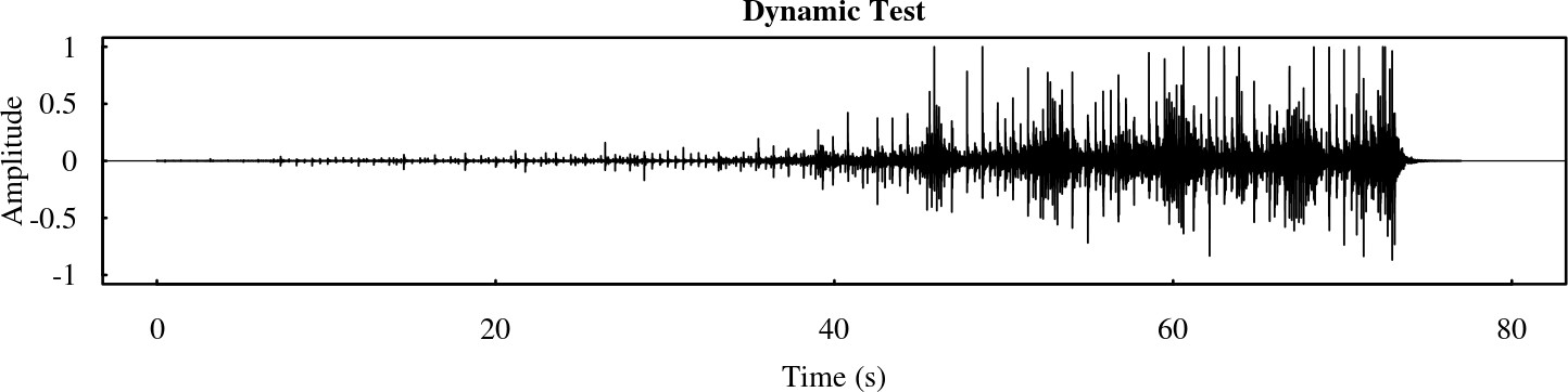
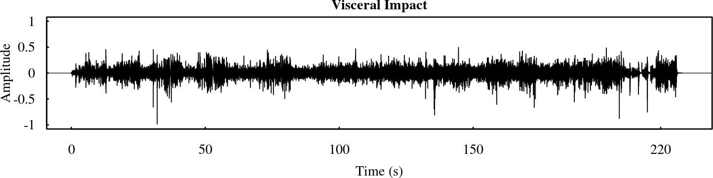
Figure 5: Waveforms of the left channel of the songs titled “Dynamic Test” (track no.29), and “Visceral Impact” (track no.17) from the audiophile CD “Ultimate Demonstration Disc: Chesky Records’ Guide to Critical Listening” (Chesky Record, catalog no. UD95).

A common way of assessing a statistical procedure is to simulate data from a certain known stochastic process fixed as the reference truth, and then compute Monte Carlo expectations of bias and efficiency measures. The problem here is that writing down a stochastic model capable of reproducing the features of real-world music signal is too complex. Instead of simulating such a signal we assess our methods based on simulated perturbations on real data. We considered two well recorded songs and we added various degrees of dynamic compression to assess whether our measure is able to highlight dynamic differences. A good method for estimating a measure of DR should consistently measure the loss of DR introduced by compressing the dynamic. In order to achieve a fair comparison we need songs on which little amount of digital processing has been applied. Chesky Records is a small label specialized in audiophile recordings, their “Ultimate Demonstration Disc: Chesky Records’ Guide to Critical Listening” (catalog number UD95), is almost a standard among audiophiles as test source for various aspects of hifi reproduction. We consider the left channel of tracks no.29, called “Dynamic Test”, and track no.17 called “Visceral Impact”. Both waveforms are reported in Figure 5. The “Dynamic Test” consists of a drum recorded near field played with an increasing level. Its sound power is so huge that a voice message warns against play backs at deliberately high volumes, which in fact could cause equipment and hearing damages. Most audiophiles subjectively consider this track as one of the most illustrious example of dynamic recording. The track is roughly one minute long. The “Visceral Impact” is actually the song “Sweet Giorgia Brown” by Monty Alexander and elsewhere published in the Chesky catalog. The song has an energetic groove from the beginning to the end and it’s about three minutes long. Differently from the previous track, that has increasing level of dynamic, this song has a uniform path. This can be clearly seen in Figure 5.

We removed initial and final silence from both tracks, and the final length (in sample units) for “Dynamic Test” is $n=2,646,000$, while $n=7,938,000$ for the second song. We then applied compression on both waves. A dynamic compressor is a function that whenever the original signal exceeds a given power (threshold parameter), the power of the output is scaled down by a certain factor (compression ratio parameter). With a threshold of -12dBFS and a compression ratio of 1.5, whenever the signal power is above -12dBFS, the compressor reduces the signal level to $2/3$ so that the input power is 1.5${\times}$(output power). All this has been performed using SoX, an high quality audio digital processing software, with all other tuning parameters set at default values. For both threshold levels equal to -12dBFS and -24dBFS we applied on each song compression ratios equal to $\{1.5,2,2.5,3,3.5,4,4.5,5\}$. There are a total of 16 compressed versions of the original wave for each song. Hence the total number of tracks involved in the simulation experiment is 34. Even though the random subsampling makes the computational effort feasible, 34 cases still require a considerable amount of computations. The subsampling algorithm has been run with $K=500$ for both songs, while $b=2205$ (which means 50ms) for “Dynamic Test”, and $b=3528$ (which means 80ms) for “Visceral Impact”. A larger $b$ for larger $n$ obeys the theoretical requirements that $b/n\rightarrow 0$ as $n$ and $b$ grow to $\infty$. The constant $M$ is fixed according to Proposition 1, i.e. $M=\lfloor\sqrt{n\hat{h}}\rfloor$. Stability analysis has been conducted changing these parameters. In particular, we tried several values of $b$ for both tracks, but results did not change overall. A larger value of $K$ also had almost no impact on the final results, however larger $K$ increases the computational load considerably. In a comparison like this, one can choose to fix the seeds for all cases so that statistics are computed over the same subsamples in all cases. However this would not allow to assess the stability of the procedure against subsampling induced variance. The results presented here are obtained with different seeds for each case, but fixed seed has been tested and it did not change the main results. Moreover, we estimate $s(\cdot)$ in $(h,1-h)$ to avoid the well known issue of the boundary effect for the kernel estimator.

Figure 6: MeSDR statistics for the song “Dynamic Test”. The left plot reports 90%-confidence bands, while the right plot reports 95%-confidence bands.

Figure 7: MeSDR statistics for the song “Visceral Impact”. The left plot reports 90%-confidence bands, while the right plot reports 95%-confidence bands.

The results for all the cases are summarized in Figures 6 and 7 where we report MeSDR statistics with 90% and 95%-confidence bands. The simulation experiment reveals an interesting evidence.

1. First notice that each of the curves in Figures 6 and 7 well emulates the theoretical behaviour of DR vs compression ratios. In fact, if we had an ideal input signal with constant unit RMS power, the DR decreases at the speed of $\log_{10}(1/\text{compression ratio})$ for any threshold value. When the RMS power is not constant, a consistent DR statistics should still behave similar to $\log_{10}(1/\text{compression ratio})$ with a curvature that depends both on the threshold parameter and the amount of power above the threshold.

2. At both threshold levels, for both songs the MeSDR does a remarkable discrimination between compression levels. For a given positive compression level none confidence bands for the -12dBFS threshold overlaps with the confidence bands for the -24dBFS case. Over 32 cases, a single overlap happens in Figure 6 for compression ratio equal to 1.5 when consider the wider 95%–confidence interval.

3. For both songs the confidence intervals are larger for the -12dBFS case, and on average the “Dynamic Test” reports longer intervals. This is expected because increasing the threshold from -12dBFS to -24dBFS will increase the proportion of samples affected by compression so that the variations of MeSDR will be reduced. Moreover we also expect that if the dynamic of a song doesn’t have a sort of uniform path, as in the case of the “Dynamic Test”, the variability of the MeSDR will be larger. Summarizing, not only the level of MeSDR, but also the length of the bands (i.e. the uncertainty) revels important information on the DR.

4. There is a smooth transition going from 90% to 95%–confidence intervals.This is an indication that the tails of the distribution of the MeSDR are well behaved.

The experiment above shows how MeSDR is able to detect consistently even small differences in compression levels. Hence it can be used to effectively discriminate between recording quality.

Figure 8: TT-DR statistics for the song “Dynamic Test” (left) and “Visceral Impact” (right).

In order to compare the results with state of the art existing methods we computed the TT-DR on the same data. The TT-DR is a popular measure of dynamic range expressed in dBFS that has gained a massive following. It is is promoted by the “Pleasurize Music Foundation” (www.pleasurizemusic.com). TT-DR is based on the sequential windowing of the signal as for the DRs, but different from this, it replaces the average power with the average of the power measurements exceeding the 80% quantile of the distribution. The idea behind the TT-DR is that compression only affects the tail of the power distribution. Results are reported in Figure 8. For the uncompressed cases the TT-DR quantifies the dynamic of “Dynamic Test” as larger than that of “Visceral Impact”, although it is clear that the “Dynamic Test” sounds more dynamic. This is because the TT-DR compares the mean of the 20% largest power measurements with the peak. The problem here is that the mean will be pushed toward the peak if within the top 20% power measurements there is still an high degree of positive asymmetry. The latter will happen particularly in cases where the dynamic variations are as extreme as for the “Dynamic Test”. A major drawback of TT-DR is that overall the range of the statistic across these cases does not exceeds 4dBFS for the “Dynamic Test”, and 8dBFS for the “Visceral Impact”, which is an indication of the inability to capture the DR concept consistently as the variations in dynamic levels here are enormous. For a given compression ratio the TT-DR does not always discriminate between the -12dBFS and the -24dBFS thresholds, and overall the differences for the two curves never exceeds 1dBFS. For a given threshold the TT-DR often fails to distinguish compression ratios, and again it is strange that this happens more for the “Dynamic Test”. The other disadvantage of the TT-DR is that the sequential windowing (deterministic) does not allow to construct confidence intervals and other inference tools.

7 Real data application

There are a number small record labels that gained success issuing remastered versions of famous albums. Some of these reissues are now out of catalogue and are traded at incredible prices on the second hand market. That means that music lovers actually value the recording quality. On the other hand majors keep issuing new remastered versions promising miracles, they often claim the use of new super technologies termed with spectacular names. But music lovers are often critical. Despite the marketing trend of mastering music with obscene levels of dynamic compression to make records sounding louder, human ears perceive dynamic compression better than it is thought. In this section we measure the DR of three different digital masterings of the song “In the Flesh?” from “The Wall” album by Pink Floyd. The album is considered one of the best rock recording of all times and “In the Flesh?” is a champion in dynamic, especially in the beginning (as reported in Figure  1) and at the end. We analysed three different masters: the MFSL by Mobile Fidelity Sound Lab (catalog UDCD 2-537, issued in 1990); EMI94 by EMI Records Ltd (catalog 8312432, issued in 1994); EMI01 produced by EMI Music Distribution (catalog 679182, issued in 2001). There are much more remasters of the album not considered here. The EMI01 has been marketed as a remaster with superior sound obtained with state of the art technology. The MFSL has been worked out by a company specialized in classic album remasters. The first impression is that the MFSL sounds softer than the EMI versions. However, there are Pink Floyd fans arguing that the MFSL sounds more dynamic, and overall is better than anything else. Also the difference between the EMI94 and EMI01 is often discussed on internet forums with fans arguing that EMI01 did not improve upon EMI94 as advertised.

Table 1: MeSDR statistics for “In the Flesh?” from “The Wall” album by Pink Floyd. “Lower” and “Upper” columns are limits of the confidence intervals based on the asymptotic approximation of the distribution of the empirical quantiles.

Seed number	Version	MeSDR	90%–Interval		95%–Interval
			Lower	Upper	Lower	Upper
Equal	MFSL	29.77	29.32	30.29	29.22	30.35
	EMI94	25.96	25.65	26.48	25.38	26.61
	EMI01	26.00	25.66	26.52	25.40	26.67
Unequal	MFSL	29.55	29.31	29.94	29.27	30.22
	EMI94	25.63	25.36	26.11	25.20	26.18
	EMI01	25.81	25.52	26.18	25.48	26.34

We measured the MeSDR of the three tracks and compared the results. Since there was a large correlation between the two channels, we only measured the channel with the largest peak, that is the left one. The three waves have been time–aligned, and the initial and final silence has been trimmed. The MeSDR has been computed with a block length of $b=2205$ (that is 50ms), and $K=500$. We computed the MeSDR both with equal and unequal seeds across the three waves to test for subsampling induced variability when $K$ is on the low side. Results are summarized in Table 1. First notice the seed changes the MeSDR only slightly. Increasing the value of $K$ to 1000 would make this difference even smaller. The second thing to notice is that MeSDR reports almost no difference between EMI94 and EMI01. In a way the figure provided by the MeSDR is consistent with most subjective opinions that the MFSL, while sounding softer, has more dynamic textures. We recall here that a 3dBFS difference is about twice the dynamic in terms of power. Table 1 suggests that the MFSL remaster is about 4dBFS more dynamic than competitors, this is a huge difference.

A further question is whether there are statistically significant differences between the sound power distributions of the tracks. It’s obvious that the descriptive nature of the approaches described in Section 2 cannot answer to such a question. Our subsampling approach can indeed answer to this kind of question by hypothesis testing. If the mixing coefficients of $\{\varepsilon_{t}\}_{t\in\mathbb{Z}}$ go to zero at a proper rate, one can take the loudness measurements $\left\{\text{DR}_{n,b,I_{i}}\quad i=1,2,\ldots,K\right\}$ as almost asymptotically independent and then apply some standard tests. In order to assess the differences in MeSDR across the three masterings we performed the Mood’s median test (Mood, 1954). The null hypothesis is that all masterings have the same MeSDR against the alternative that at least one of them is different. We used $\text{DR}_{n,b,I_{i}}$ estimates from unequal seed calculations to reinforce the independence between the three groups. The resulting p-value is 8.95${\times}10^{-17}$, the latter confirms the subjective perception that there are strong differences. Performing the Mood’s test in pairs, the p-value is extremely low when MFSL is compared against EMI94 or EMI01, while the comparison between EMI94 and EMI01 gives a p-value=0.6579907. Although the median test here is a natural choice, Freidlin and Gastwirth (2000) showed that it has low power in many situations. The suggestion of Freidlin and Gastwirth (2000) for two-sample problems is to use the Mann-Whitney tests for location shift. Therefore, we applied the Mann-Whitney test for the null hypothesis that the DR distribution of MFSL and EMI94 are not location-shifted, against the alternative that MFSL is right shifted with respect to EMI94. The resulting p-value$<2.2\times 10^{-16}$ suggests to reject the null at any sensible significance level, and this confirms that MFSL sounds more dynamic compared to EMI94. Comparison between MFSL and EMI01 leads to a similar result. We also tested the null hypothesis that EMI94 and EMI01 DR levels are not location-shifted, against the alternative that there is some shift different from zero. The resulting p-value=0.6797 suggests to not reject the null at any standard confidence level. The latter confirms the figure suggested by MeSDR, that is, there is no significant overall dynamic difference between the two masterings.

8 Concluding Remarks

Starting from the DR problem we exploited a novel methodology to estimate the variance distribution of a time series produced by a stochastic process additive to a smooth function of time. The general set of assumptions on the error term makes the proposed model flexible and general enough to be applied under various situations not explored in this paper. The smoothing and the subsampling theory is developed for fixed global bandwidth and fixed subsample size. We constructed a DR statistic that is based on the random term. This has two main advantages: (i) it allows to draw conclusions based on inference; (ii) since power variations are about sharp changes in the energy levels, it is likely that these changes will affect the stochastic part of (5) more than the smooth component. In a controlled experiment our DR statistic has been able to highlight consistently dynamic range compressions. Moreover we provided an example where the MeSDR statistic is able to reconstruct differences perceived subjectively on real music signals.

Appendix

Proof of Proposition 1.

First notice that A2–A3 in this paper imply that Assumptions A–E in Altman (1990) are fulfilled. In particular A2 on mixing coefficients of $\varepsilon_{t}$ ensures that Assumptions E and D in Altman (1990) are satisfied. Let $\hat{\gamma}(j)=\frac{1}{n}\sum_{t=1}^{n-j}\hat{\varepsilon}_{t}\hat{\varepsilon}_{t+j}$ be the estimator of the autocovariance $\gamma(j)$ with $j=0,1,\ldots$ and $r_{n}=\frac{1}{nh}+h^{4}=n^{-4/5}$ by A3. First we note that by Markov inequality

$$\frac{1}{n}\sum_{i=1}^{n}\left(s(i/n)-\hat{s}(i/n)\right)^{2}-\text{MISE}(h;\hat{s})=o(r_{n})$$ (11)

Let us now rearrange $\hat{\gamma}(j)$ as

$$\hat{\gamma}(j) = \frac{1}{n}\sum_{i=1}^{n-j}\left(s(i/n)-\hat{s}(i/n)\right)\left(s((i+j)/n)-\hat{s}((i+j)/n)\right)+$$ (12)

$$+ \frac{1}{n}\sum_{i=1}^{n-j}\left(s((i+j)/n)-\hat{s}((i+j)/n)\right)\varepsilon_{i}+$$

$$+ \frac{1}{n}\sum_{i=1}^{n-j}\left(s(i/n)-\hat{s}(i/n)\right)\varepsilon_{i+j}+\frac{1}{n}\sum_{i=1}^{n-j}\varepsilon_{i}\varepsilon_{i+j}=I+II+III+IV$$

By (11) and Schwartz inequality it results that $I=O_{p}\left(r_{n}\right)$. Now, consider term $III$ in (12). Since $\hat{s}(t)=s(t)\left(1+O_{p}\left(r_{n}^{1/2}\right)\right)$, it is sufficient to investigate the behaviour of

$$\frac{1}{n}\sum_{i=1}^{n-j}s(i/n)\varepsilon_{i+j}.$$

By A1 and applying Chebishev inequality, it happens that $III=O_{p}(n^{-1/2})$. Based on similar arguments one has that term $II=O_{p}(n^{-1/2})$. Finally, $IV=\gamma(j)+O_{p}(n^{-1/2})$. Then $\hat{\gamma}(j)=\gamma(j)+O_{p}(r_{n})+O_{p}(n^{-1/2})+O_{p}(j/n)$, where the $O_{p}(j/n)$ is due to the bias of $\hat{\gamma}(j)$. It follows that also $\hat{\rho}(j)=\rho(j)+O_{p}(r_{n})+O_{p}(n^{-1/2})+O_{p}(j/n)$. Since $\mathcal{K}(\cdot)$ is bounded from above then one can write

$$\frac{1}{nh}\sum_{j=-M}^{M}\mathcal{K}\left(\frac{j}{nh}\right)\hat{\rho}(j)= \frac{1}{nh}\sum_{j=-M}^{M}\mathcal{K}\left(\frac{j}{nh}\right)\rho(j)+$$

$${}+ \frac{M}{nh}O_{p}(r_{n})+\frac{M}{nh}O_{p}(n^{-1/2})+\frac{M^{2}}{n}O_{p}\left(\frac{1}{nh}\right);$$

by A4 and $h=O(n^{-1/5})$, it holds true that

$$\frac{1}{nh}\sum_{j=-M}^{M}\mathcal{K}\left(\frac{j}{nh}\right)\hat{\rho}(j)=\frac{1}{nh}\sum_{j=-M}^{M}\mathcal{K}\left(\frac{j}{nh}\right)\rho(j)+o_{p}(r_{n}).$$ (13)

So, taking the quantity in the expression (22) of Altman (1990), we have to evaluate

$$Q_{1}=\left|\frac{1}{nh}\sum_{j=-nh/2}^{nh/2}\mathcal{K}\left(\frac{j}{nh}\right)\rho(j)-\frac{1}{nh}\sum_{j=-M}^{M}\mathcal{K}\left(\frac{j}{nh}\right)\hat{\rho}(j)\right|$$

where we consider the nearest integer in place of $nh$. By (13), it follows that

$$Q_{1}=\left|\frac{2}{nh}\sum_{j=M+1}^{nh/2}\mathcal{K}\left(\frac{j}{nh}\right)\rho(j)\right|+o_{p}(r_{n}).$$

Since, by assumptions A2, A3 and A4,

$$\frac{1}{nh}\sum_{j=M+1}^{nh/2}\mathcal{K}\left(\frac{j}{nh}\right)\rho(j)\sim\rho(nh)=o(r_{n}),$$

then $Q_{1}=o_{p}(r_{n})$. Notice that the first term in $Q_{1}$ is the analog of expression (22) in Altman (1990). Therefore, $\text{CV}(h)$ can now be written as

$$\text{CV}(h) =\left[1-\frac{1}{nh}\sum_{j=-M}^{M}\mathcal{K}\left(\frac{j}{nh}\right)\hat{\rho}(j)\right]^{-2}\frac{1}{n}\sum_{i=1}^{n}\hat{\varepsilon}_{i}^{2}$$

$$=\left[1-\frac{1}{nh}\sum_{j=-nh/2}^{nh/2}\mathcal{K}\left(\frac{j}{nh}\right)\rho(j)\right]^{-2}\frac{1}{n}\sum_{i=1}^{n}\hat{\varepsilon}_{i}^{2}+o_{p}(r_{n}).$$

Apply the classical bias correction and based on (14) in Altman (1990), we have that

$$\text{CV}(h)=\frac{1}{n}\sum_{t=1}^{n}\varepsilon_{t}^{2}+\text{MISE}(h;\hat{s})+o_{p}(r_{n}),$$

using the same arguments as in the proof of Theorem 1 in Chu and Marron (1991). Since $\text{MISE}(h;\hat{s})=O(r_{n})$, it follows that $\hat{h}$, the minimizer of $\text{CV}(h)$, is equal to $h^{\star}$, the minimizer of $\text{MISE}(h;\hat{s})$, asymptotically in probability. ∎

Before proving Proposition 2, we need a technical Lemma that states the consistency of the classical subsampling (not random) in the case of the estimator $\hat{s}(t)$ on the entire sample.

Lemma 1.

Assume A1, A2, A3 and A4. Let $\hat{s}(t)$ be the estimator of $s(t)$ computed on the entire sample (of length n). If $b/n\rightarrow 0$ whenever $n\rightarrow\infty$and $b\rightarrow\infty$, then

$$(i) \sup_{x}\left|\hat{G}_{n,b}(x)-G(x)\right|\stackrel{{\scriptstyle p}}{{\longrightarrow}}0$$

$$(ii) \hat{q}_{n,b}(\gamma)\stackrel{{\scriptstyle p}}{{\longrightarrow}}q(\gamma)$$

where $\gamma\in(0,1)$ and $\hat{G}_{n,b}(x)$, $G(x)$, $\hat{q}_{n,b}(\gamma)$ and $q(\gamma)$ are defined in Section 4.

Proof.

For the part (i), notice that under the assumption A2, the conditions of Theorem (4.1) in Politis et al. (2001) hold. Let us denote $r_{n}=\frac{1}{nh}+h^{4}$, which is $r_{n}=n^{-4/5}$ by Proposition (1). As in the proof of Proposition (1), we can write

$$\frac{1}{b}\sum_{i=t}^{t+b-1}\left(\hat{\varepsilon}_{i}-\varepsilon_{i}\right)^{2}=O_{p}(r_{n})+O(1/b)\qquad\text{for all}\;t,$$

since $\hat{s}(\cdot)$ is estimated on the entire sample of length $n$ and $\{\varepsilon_{i}\}$ is a sequence of stationary random variables by A2. The term $O(1/b)$ is due to the error of the deterministic variable in $s(\cdot)$, when we consider the mean instead of the integral. Note that we do not report this error ($O(1/n)$) in (11) because the leading term is $r_{n}$ given that $r_{n}^{-1}/n\rightarrow 0$ when $n\rightarrow\infty$. In this case $b^{-1}\sum_{i=t}^{t+b-1}\left(\hat{\varepsilon}_{i}-\varepsilon_{i}\right)^{2}$ is an estimator of $\text{MISE}_{I}(h;\hat{s})$ on a set $I\subset(0,1)$. Now $\sqrt{b}(r_{n}+b^{-1})\rightarrow 0$ as $n\rightarrow\infty$, and all this is sufficient to have that $\sqrt{b}\left(\hat{V}_{n,b,t}-V_{n,b,t}\right)\stackrel{{\scriptstyle\text{p}}}{{\longrightarrow}}0$, for all $t$. Then, we can conclude that $\sqrt{b}\left(\hat{V}_{n,b,t}-V_{n}\right)$ has the same asymptotic distribution as $\sqrt{b}\left(V_{n,b,t}-V_{n}\right)$. Let us denote $Z_{1t}=\sqrt{b}\left(V_{n,b,t}-V_{n}\right)$ and $Z_{2t}=\sqrt{b}\left(\hat{V}_{n,b,t}-V_{n,b,t}\right)$, hence

$$\hat{G}_{n,b}(x)=\frac{1}{n-b+1}\sum_{t=1}^{n-b+1}\text{\bf\large 1}\left\{Z_{1t}+Z_{2t}\leq x\right\}.$$

By the same arguments used for the proof of Slutsky theorem the previous equation can be written as

$$\sup_{x}\left|\hat{G}_{n,b}(x)-G(x)\right| \leq \sup_{x}\left|G_{n,b}(x\pm\xi)-G(x)\right|+$$

$$+ \frac{1}{n-b+1}\sum_{t=1}^{n-b+1}\text{\bf\large 1}\left\{|Z_{2t}|>\xi\right\}$$

for any positive constant $\xi$. Since $G(x)$ is continuous at any $x$ (Normal distribution), it follows that $\sup_{x}\left|G_{n,b}(x)-G(x)\right|\stackrel{{\scriptstyle\text{p}}}{{\longrightarrow}}0$ by Theorem (4.1) in Politis et al. (2001). Moreover, by A2 $Z_{2t}\stackrel{{\scriptstyle\text{p}}}{{\longrightarrow}}0$, for all $t$ and thus

$$\frac{1}{n-b+1}\sum_{t=1}^{n-b+1}\text{\bf\large 1}\left\{|Z_{2t}|>\xi\right\}\stackrel{{\scriptstyle\text{p}}}{{\longrightarrow}}0,$$

for all $\xi>0$, which proves the result.

Finally, part (ii) is straightforward following Theorem 5.1 of Politis et al. (2001) and part (i) of this Lemma. ∎

Proof of Proposition 2.

Let $\mbox{P}^{*}(X)$ and $\mbox{E}^{*}(X)$ be the conditional probability and the conditional expectation of a random variable $X$ with respect to a set $\chi=\left\{Y_{1},\ldots,Y_{n}\right\}$. Here $\hat{G}_{n,b}(x)$ uses the estimator $\hat{s}_{b}(\cdot)$ on each subsample of length $b$. Then,

$$\frac{1}{b}\sum_{i=t}^{t+b-1}\left(\hat{\varepsilon}_{i}-\varepsilon_{i}\right)^{2}=O_{p}\left(b^{-4/5}\right)\qquad\text{for all}\;t,$$

as in the proofs of Proposition 1 and Lemma 1 (i). Then, $\sqrt{b}b^{-4/5}\rightarrow 0$. So, by Lemma 1 (i), it follows that

$$\sup_{x}\left|\hat{G}_{n,b}(x)-G(x)\right|\stackrel{{\scriptstyle\text{p}}}{{\longrightarrow}}0,$$

since $G(x)$ is continuous for all $x$. Let $Z_{i}(x)=\text{\bf\large 1}\left\{\sqrt{b}\left(\hat{V}_{n,b,i}-V_{n}\right)\leq x\right\}$ and $Z_{i}^{*}(x)=\text{\bf\large 1}\left\{\sqrt{b}\left(\hat{V}_{n,b,I_{i}}-V_{n}\right)\leq x\right\}$. $I_{i}$ is a random variable from $I=\left\{1,2,\ldots,n-b+1\right\}$. Then, $\mbox{P}^{*}(Z_{i}^{*}(x)=Z_{i}(x))=\frac{1}{n-b+1}$ for all $i$ and each $x$. Then, we can write $\tilde{G}_{n,b}(x)=\frac{1}{K}\sum_{i=1}^{K}Z_{i}^{*}(x)$ and

$$\mbox{E}^{*}\left(\tilde{G}_{n,b}(x)\right)=\frac{1}{n-b+1}\sum_{t=1}^{n-b+1}Z_{i}(x)=\hat{G}_{n,b}(x)\stackrel{{\scriptstyle\text{p}}}{{\longrightarrow}}G(x).$$

By Corollary 2.1 in Politis and Romano (1994) we have that

$$\sup_{x}\left|\tilde{G}_{n,b}(x)-\hat{G}_{n,b}(x)\right|\rightarrow 0\quad\mbox{almost sure}.$$

Then, the result follows. ∎

Proof of Corollary 1.

It follows the proof of Lemma 1 (ii) by replacing Lemma 1 (i) with Proposition 2. ∎

References

- Altman (1990) Altman, N. S. (1990). Kernel smoothing of data with correlated errors. Journal of the American Statistical Association 85(411), 749–759.
- Altman (1993) Altman, N. S. (1993). Estimating error correlation in nonparametric regression. Statistics & probability letters 18(3), 213–218.
- Ballou (2005) Ballou, G. (2005). Handbook for Sound Engineers. Focal Press.
- Berg et al. (2012) Berg, A., T. McMurry, and D. N. Politis (2012). Testing time series linearity: traditional and bootstrap methods. Handbook of Statistics: Time Series Analysis: Methods and Applications 30, 27.
- Boley et al. (2010) Boley, J., M. Lester, and C. Danner (2010). Measuring dynamics: Comparing and contrasting algorithms for the computation of dynamic range. In Proceedings of the AES 129th Convention, San Francisco.
- Chu and Marron (1991) Chu, C. K. and J. S. Marron (1991). Comparison of two bandwidth selectors with dependent errors. The Annals of Statistics 19(4), 1906–1918.
- Francisco-Fernández et al. (2004) Francisco-Fernández, M., J. Opsomer, and J. M. Vilar-Fernández (2004). Plug-in bandwidth selector for local polynomial regression estimator with correlated errors. Journal of Nonparametric Statistics 16(1-2), 127–151.
- Freidlin and Gastwirth (2000) Freidlin, B. and J. L. Gastwirth (2000). Should the median test be retired from general use? The American Statistician 54(3), 161–164.
- Hall et al. (1995) Hall, P., S. N. Lahiri, and J. Polzehl (1995). On bandwidth choice in nonparametric regression with both short- and long-range dependent errors. The Annals of Statistics 23(6), 1921–1936.
- Hart (1991) Hart, J. D. (1991). Kernel regression estimation with time series errors. J. Roy. Statist. Soc. Ser. B 53(1), 173–187.
- Katz (2007) Katz, B. (2007). Mastering audio: the art and the science. Focal Press.
- Mood (1954) Mood, A. M. (1954). On the asymptotic efficiency of certain nonparametric two-sample tests. The Annals of Mathematical Statistics, 514–522.
- Politis and Romano (1994) Politis, D. N. and J. P. Romano (1994). Large sample confidence regions based on subsamples under minimal assumptions. The Annals of Statistics 22(4), 2031–2050.
- Politis and Romano (2010) Politis, D. N. and J. P. Romano (2010). K-sample subsampling in general spaces: The case of independent time series. Journal of Multivariate Analysis 101(2), 316–326.
- Politis et al. (2001) Politis, D. N., J. P. Romano, and M. Wolf (2001). On the asymptotic theory of subsampling. Statistica Sinica 11(4), 1105–1124.
- Priestley and Chao (1972) Priestley, M. and M. Chao (1972). Non-parametric function fitting. Journal of the Royal Statistical Society. Series B (Methodological) 34(3), 385–392.
- Risset and Mathews (1969) Risset, J. C. and M. V. Mathews (1969). Analysis of musical-instrument tones. Physics today 22, 23.
- Serra and Smith (1990) Serra, X. and J. Smith (1990). Spectral modeling synthesis: A sound analysis/synthesis system based on a deterministic plus stochastic decomposition. Computer Music Journal 14(4), 12.
- Vickers (2010) Vickers, E. (2010). The loudness war: Background, speculation and recommendations. In Proceedings of the AES 129th Convention, San Francisco, CA, pp. 4–7.
- von Helmholtz (1885) von Helmholtz, H. (1885). On the sensations of tone (English translation AJ Ellis). New York: Dover.
- Voss (1978) Voss, R. F. (1978). ”1/f noise” in music: Music from 1/f noise. The Journal of the Acoustical Society of America 63(1), 258.
- Voss and Clarke (1975) Voss, R. F. and J. Clarke (1975, Nov). “1/fnoise” in music and speech. Nature 258(5533), 317–318.
- Xia and Li (2002) Xia, Y. and W. Li (2002). Asymptotic behavior of bandwidth selected by the cross-validation method for local polynomial fitting. Journal of multivariate analysis 83(2), 265–287.