Cache-Oblivious Peeling of Random Hypergraphs

Abstract

The computation of a peeling order in a randomly generated hypergraph is the most time-consuming step in a number of constructions, such as perfect hashing schemes, random $r$-SAT solvers, error-correcting codes, and approximate set encodings. While there exists a straightforward linear time algorithm, its poor I/O performance makes it impractical for hypergraphs whose size exceeds the available internal memory.

We show how to reduce the computation of a peeling order to a small number of sequential scans and sorts, and analyze its I/O complexity in the cache-oblivious model. The resulting algorithm requires $O(\operatorname{sort}(n))$ I/Os and $O(n\log n)$ time to peel a random hypergraph with $n$ edges.

We experimentally evaluate the performance of our implementation of this algorithm in a real-world scenario by using the construction of minimal perfect hash functions (MPHF) as our test case: our algorithm builds a MPHF of $7.6$ billion keys in less than $21$ hours on a single machine. The resulting data structure is both more space-efficient and faster than that obtained with the current state-of-the-art MPHF construction for large-scale key sets.

1 Introduction

Hypergraphs can be used to model sets of dependencies among variables of a system: vertices correspond to variables and edges to relations of dependency among variables, such as equations binding variables together. This correspondence can be used to transfer graph-theoretical properties to solvability conditions in the original system of dependencies.

Among these, one of the most useful is the concept of peeling order. Given an $r$-hypergraph, a peeling order is an order of its edges such that each edge has a vertex of degree $1$ in the subgraph obtained by removing the previous edges in the order. Such an order exists if the hypergraph does not have a non-empty $2$-core, i.e. a set of vertices that induces a subgraph whose vertices have all degree at least $2$.

In the above interpretation, if the equations of a system are arranged in peeling order, then each equation has at least one variable that does not appear in any equation that comes later in the ordering, i.e., the system becomes triangular, so it can be easily solved by backward substitution. For this reason, peeling orders found application in a number of fundamental problems, such as hash constructions [3, 6, 9, 10, 11, 12, 21], solving random instances of $r$-SAT [12, 24, 25], and the construction of error-correcting codes [15, 20, 23]. These applications exploit the guarantee that if the edge sparsity $\gamma$ of a random $r$-hypergraph is larger than a certain sparsity threshold $c_{r}$ (e.g., $c_{3}\approx 1.221$), then with high probability the hypergraph has an empty $2$-core [25].

The construction of perfect hash functions (PHF) is probably the most important of the aforementioned applications. Given a set $S$ of $n$ keys, a PHF for $S$ maps the $n$ keys onto the set of the first $m$ natural numbers bijectively. A perfect hash function is minimal (MPHF) if $m=n=|S|$. A lower bound by Mehlhorn [22] states that $n\log e\approx 1.44n$ bits are necessary to represent a MPHF; a matching (up to lower order terms) upper bound is provided in [16], but the construction is impractical. Most practical approaches, instead, are based on random $3$-hypergraphs, resulting in MPHFs that use about $2c_{3}n\approx 2.5n$ bits [6, 10, 21]. These solutions, which we review in Section 3, build on the MWHC technique [21], whose most demanding task is in fact the computation of a peeling order.

There is a surprisingly simple greedy algorithm to find a peeling order when it exists, or a $2$-core when it does not: find a vertex of degree $1$, remove (peel) its only edge from the hypergraph, and iterate this process until either no edges are left (in which case the removal order is a peeling order), or all the non-isolated vertices left have degree at least $2$ (thus forming a $2$-core). This algorithm can be easily implemented to run in linear time and space.

MPHFs are the main ingredient in many space-efficient data structures, such as (compressed) full-text indexes [4], monotone MPHFs [1], Bloom filter-like data structures [5], and prefix-search data structures [2].

It should be clear that the applications that benefit the most from such data structures are those involving large-scale key sets, often orders of magnitude larger than the main memory. Unfortunately, the standard linear-time peeling algorithm requires several tens of bytes per key of working memory, even if the final data structure can be stored in just a handful of bits per key. It is hence common that, while the data structure fits in memory, such memory is not enough to actually build it. It is then necessary to resort to external memory, but the poor I/O performance of the algorithm makes such an approach impossible.

Application-specific workarounds have been devised; for example, Botelho et al. [6] proposed an algorithm (called HEM) to build MPHFs in external memory by splitting the key set into small buckets and computing independent MPHFs for each bucket. A first-level index is used to find the bucket of a given key. The main drawback of this solution is that the first-level index introduces a non-negligible overhead in both space and lookup time; moreover, this construction cannot be extended to applications other than hashing.

In this paper we provide the first efficient algorithm in the cache-oblivious model that, given a random $r$-hypergraph with $n$ edges and $\gamma n$ vertices (with $r=O(1)$ and $\gamma>c_{r}$), computes a peeling order in time $O(n\log n)$ and with $O(\operatorname{sort}(n))$ I/Os w.h.p., where $\operatorname{sort}(n)$ is the I/O complexity of sorting $n$ keys. By applying this result we can construct (monotone) MPHFs, static functions, and Bloom filter-like data structures in $O(\operatorname{sort}(n))$ I/Os. In our experimental evaluation, we show that the algorithm makes it indeed possible to peel very large hypergraphs: an MPHF for a set of $7.6$ billion keys is computed in less than $21$ hours; on the same hardware, the standard algorithm would not be able to manage more than $2.1$ billion keys. Although we use minimal perfect hash functions construction as our test case, results of these experiments remain valid for all the other applications due to the random nature of the underlying hypergraphs.

2 Notation and tools

Model and assumptions  We analyze our algorithms in the cache-oblivious model [14]. In this model, the machine has a two-level memory hierarchy, where the fast level has an unknown size of $M$ words and a slow level of unbounded size where our data reside. We assume that the fast level plays the role of a cache for the slow level with an optimal replacement strategy where the transfers (a.k.a. I/Os) between the two levels are done in blocks of an unknown size of $B\leq M$ words; the I/O cost of an algorithm is the total number of such block transfers. Scanning and sorting are two fundamental building blocks in the design of cache-oblivious algorithms [14]: under the tall-cache assumption [8], given an array of $N$ contiguous items the I/Os required for scanning and sorting are

$$\operatorname{scan}(N)=O\left(1+\frac{N}{B}\right)\text{ I/Os}\quad\text{and}\quad\operatorname{sort}(N)=O\left(\frac{N}{B}\log_{M/B}\frac{N}{B}\right)\text{.}$$

Hypergraphs An $r$-hypergraph on a vertex set $V$ is a subset $E$ of ${V\choose r}$, the set of subsets of $V$ of cardinality $r$. An element of $E$ is called an edge. We call an ordered $r$-tuple from $V$ an oriented edge; if $e$ is an edge, an oriented edge whose vertices are those in $e$ is called an orientation of $e$. From now on we will focus on $3$-hypergraphs; generalization to arbitrary $r$ is straightforward. We define valid orientations those oriented edges $(v_{0},v_{1},v_{2})$ where $v_{1}<v_{2}$ (for arbitrary $r$, $v_{1}<\dots<v_{r-1}$). Then for each edge there are $6$ orientations, but only $3$ valid orientations ($r!$ orientations of which $r$ are valid).

We say that a valid oriented edge $(v_{0},v_{1},v_{2})$ is the $i$-th orientation if $v_{0}$ is the $i$-th smallest among the three; in particular, the $0$-th orientation is the canonical orientation. Edges correspond bijectively with their canonical orientations. Furthermore, valid orientations can be mapped bijectively to pairs $(e,v)$ where $e$ is an edge and $v$ a vertex contained in $e$, simply by the correspondence $(v_{0},v_{1},v_{2})\mapsto(\{v_{0},v_{1},v_{2}\},v_{0})$. In the following all the orientations are assumed to be valid, so we will use the term orientation to mean valid orientation.

3 The Majewski–Wormald–Havas–Czech technique

Majewski et al. [21] proposed a technique (MWHC) to compute an order-preserving minimal perfect hash function, that is, a function mapping a set of keys $S$ in some specified way into $[|S|]$. The technique actually makes it possible to store succinctly any function $f:S\to[\sigma]$, for arbitrary $\sigma$. In this section we briefly describe their construction.

First, we choose three random hash functions $h_{0},h_{1},h_{2}:S\to[\gamma n]$ and generate a 3-hypergraph with $\gamma n$ vertices, where $\gamma$ is a constant above the critical threshold $c_{3}$ [25], by mapping each key $x$ to the edge $\{h_{0}(x),h_{1}(x),h_{2}(x)\}$. The goal is to find an array $u$ of $\gamma n$ integers in $[\sigma]$ such that for each key $x$ one has $f(x)=u_{h_{0}(x)}+u_{h_{1}(x)}+u_{h_{2}(x)}\mod\sigma$. This yields a linear system with $n$ equations and $\gamma n$ variables $u_{i}$; if the associated hypergraph is peelable, it is easy to solve the system. Since $\gamma$ is larger than the critical threshold, the algorithm succeeds with probability $1-o(1)$ as $n\to\infty$ [25].

By storing such values $u_{i}$, each requiring $\lceil\log\sigma\rceil$ bits, plus the three hash functions, we will be able to recover $f(x)$. Overall, the space required will be $\lceil\log\sigma\rceil\gamma n$ bits, which can be reduced to $\lceil\log\sigma\rceil n+\gamma n+o(n)$ using a ranking structure [17]. This technique can be easily extended to construct MPHFs: we define the function $f\colon S\to[3]$ as $x\mapsto i$ where $h_{i}(x)$ is a degree-$1$ vertex when the edge corresponding to $x$ is peeled; it is then easy to see that $h_{f(x)}(x):S\to[\gamma n]$ is a PHF. The function can be again made minimal by adding a ranking structure on the vector $u$ [6].

As noted in the introduction, the peeling procedure needed to solve the linear system can be performed in linear time using a greedy algorithm (referred to as standard linear-time peeling). However, this procedure requires random access to several integers per key, needed for bookkeeping; moreover, since the graph is random, the visit order is close to random. As a consequence, if the key set is so large that it is necessary to spill to the disk part of the working data structures, the I/O volume slows down the algorithm to unacceptable rates.

Practical workarounds (HEM) Botelho et al. [6] proposed a practical external-memory solution: they replace each key with a signature of $\Theta(\log n)$ bits computed with a random hash function, so that no collision occurs. The signatures are then sorted and divided into small buckets based on their most significant bits, and a separate MPHF is computed for each bucket with the approach described above. The representations of the bucket functions are then concatenated into a single array and their offsets stored in a separate vector.

The construction algorithm only requires to sort the signatures (which can be done efficiently in external memory) and to scan the resulting array to compute the bucket functions; hence, it is extremely scalable. The extra indirection needed to address the blocks causes however the resulting data structure to be both slower and larger than one obtained by computing a single function on the whole key set. In their experiments with a practical version of the construction, named HEM, the authors report that the resulting data structure is $21\%$ larger than the one built with plain MWHC, and lookups are $30\text{--}50\%$ slower. A similar overhead was confirmed in our experiments, which are discussed in Section 5.

4 Cache-oblivious peeling

In this section we describe a cache-oblivious algorithm to peel an $r$-hypergraph. We describe the algorithm for $3$-hypergraphs, but it is easy to generalize it to arbitrary $r$.

4.1 Maintaining incidence lists

In order to represent the hypergraph throughout the execution of the algorithm, we need a data structure to store the incidence list of every vertex $v_{0}$, i.e., the list $L_{v_{0}}=\{(v_{0},v_{1}^{0},v_{2}^{0}),\allowbreak\dots,\allowbreak(v_{0},v_{1}^{d-1},v_{2}^{d-1})\}$ of valid oriented edges whose first vertex is $v_{0}$. To realize the peeling algorithm, it is sufficient to implement the following operations on the lists.

• $\operatorname{Degree}(L_{v_{0}})$ returns the number of edges $d$ in the incidence list of $v_{0}$;

• $\operatorname{AddEdge}(L_{v_{0}},e)$ adds the edge $e$ to the incidence list of $v_{0}$;

• $\operatorname{DeleteEdge}(L_{v_{0}},e)$ deletes the edge $e$ from the incidence list of $v_{0}$;

• $\operatorname{RetrieveEdge}(L_{v_{0}})$ returns the only edge in the list if $\operatorname{Degree}(L_{v_{0}})=1$.

For all the operations above, it is assumed that the edge is given through a valid orientation. Under this set of operations, the data structure does not need to store the actual list of edges: it is sufficient to store a tuple $(v_{0},d,\tilde{v}_{1},\tilde{v}_{2})$, where $d$ is the number of edges, $\tilde{v}_{1}=\bigoplus_{j<d}v_{1}^{j}$, and $\tilde{v}_{2}=\bigoplus_{j<d}v_{2}^{j}$, that is, all the vertices of the list in the same position are XORed together.

The operations $\operatorname{AddEdge}$ and $\operatorname{DeleteEdge}$ on an edge $(v_{0},v_{1}^{\prime},v_{2}^{\prime})$ simply XOR $v_{1}^{\prime}$ into $\tilde{v}_{1}$ and $v_{2}^{\prime}$ into $\tilde{v}_{2}$, and respectively increment or decrement $d$. Since all the edges are assumed valid (i.e., it holds that $v_{1}^{\prime}<v_{2}^{\prime}$) these operations maintain the invariant. When $d=1$, clearly $\tilde{v}_{1}=v_{1}$ and $\tilde{v}_{2}=v_{2}$ where $(v_{0},v_{1},v_{2})$ is the only edge in $L_{v_{0}}$, so it can be returned by $\operatorname{RetrieveEdge}$. If necessary, the data structure can be trivially extended to labeled edges $(v_{0},v_{1},v_{2},\ell)$ by XORing together the labels $\ell$ into a new field $\tilde{\ell}$.

We call this data structure packed incidence list, and we refer to this technique as the XOR trick. The advantage with respect to maintaining an explicit list, besides the obvious space savings, is that it is sufficient to maintain a single fixed-size record per vertex, regardless of the number of incident edges. This will make the peeling algorithm in the next section substantially simpler and faster. The same trick can be applied to the standard linear-time algorithm, replacing the linked lists traditionally used. As we will see in Section 5, the improvements are significant in both working space and running time.

4.2 Layered peeling

The peeling procedure we present is an adaptation of the CORE procedure presented by Molloy [25]. The basic idea is to proceed in rounds: at each round, all the vertices of degree $1$ are removed, and then the next round is performed on the induced subgraph, until either a $2$-core is left, or the graph is empty. In the latter case, the algorithm partitions the edges into a sequence of layers, one per round, by defining each layer as the set of edges removed in its round. It is easy to see that by concatenating the layers the resulting edge order is a peeling order, regardless of the order within each layer.

The layered peeling process terminates in a small number of rounds: Jiang et al. [18] proved that if the hypergraph is generated randomly with a sparsity above the peeling threshold, then with high probability the number of rounds is bounded by $O(\log\log n)$. Moreover, the fraction of vertices remaining in each round decreases double-exponentially. In the following we show how to implement the algorithm in an I/O-efficient way by putting special care in the hypergraph representation and the update step.

Hypergraph representation At each round $i$, the hypergraph is represented by a list $E_{i}$ of tuples $(v_{0},d,\tilde{v}_{1},\tilde{v}_{2})$ as described in Section 4.1; each tuple represents the incidence list of $v_{0}$. Each list $E_{i}$ is sorted by $v_{0}$. Note that each edge $e=\{v_{0},v_{1},v_{2}\}$ needs to be in the incidence list of all its vertices; hence, all the three orientations of $e$ are present in the list $E_{i}$.

Construction of $E_{0}$ To construct $E_{0}$, the edge list for the first round, we put together in a list all the valid orientations of all the edges in the hypergraph. The list is then sorted by $v_{0}$, and from the sorted list we can construct the sorted list of incidence lists $E_{0}$: after grouping the oriented edges by $v_{0}$, we start with the empty packed incidence list $(v_{0},0,0,0)$ and, after performing $\operatorname{AddEdge}$ with all the edges in the group, we append it to $E_{0}$. The I/O complexity is $O(\operatorname{sort}(n)+\operatorname{scan}(n))=O(\operatorname{sort}(n))$.

Round update At the beginning of each round we are given the list $E_{i}$ of edges that are alive at round $i$, and we produce $E_{i+1}$. We first scan $E_{i}$ to find all the tuples $L$ such that $\operatorname{Degree}(L)=1$; for each tuple, we perform $\operatorname{RetrieveEdge}$ and put the edge in a list $D_{i}$, which represents all the edges to be removed in the current round $i$. The same edge may occur multiple times in $D_{i}$ under different orientations (if more than one of its vertices have degree $1$ in the current round); to remove the duplicates, we sort the oriented edges by their canonical orientation, keep one orientation for each edge, and store them in a list $P_{i}$.

Now we need to remove the edges from the hypergraph. To do so, we generate a degree update list $U_{i}$ that contains all the three orientations for each edge in $P_{i}$, and sort $U_{i}$ by $v_{0}$. Since both $E_{i}$ and $U_{i}$ are sorted by $v_{0}$, we can scan them both simultaneously joining them by $v_{0}$; for each tuple $L_{v_{0}}$ in $E_{i}$, if no oriented edge starting with $v_{0}$ is in $U_{i}$ the tuple is copied to $E_{i+1}$, otherwise for each such oriented edge $e$, $\operatorname{DeleteEdge}(L_{v_{0}},e)$ is called to obtain a new $L_{v_{0}}^{\prime}$ which is written to $E_{i+1}$ if non-empty. Note that $E_{i+1}$ remains sorted by $v_{0}$.

For each round, we scan $E_{i}$ twice and $U_{i}$ once, and sort $D_{i}$ and $U_{i}$. The number of I/Os is then $2\cdot\operatorname{scan}(|E_{i}|)+\operatorname{scan}(|U_{i}|)+\operatorname{sort}(|D_{i}|)+\operatorname{sort}(|U_{i}|)$. Summing over all rounds, we have $\sum_{i}(2\cdot\operatorname{scan}(|E_{i}|)+\operatorname{sort}(|D_{i}|)+\operatorname{sort}(|U_{i}|)+\operatorname{scan}(|U_{i}|))=O(\operatorname{sort}(n))$ because each edge belongs to at most three lists $D_{i}$ and three lists $U_{i}$. Since the fraction of vertices remaining at each round decreases doubly exponentially and, thanks to the XOR trick, $E_{i}$ has exactly a tuple for each vertex alive in the $i$-th round, the cost of scanning the lists $E_{i}$ sums up to $O(\operatorname{scan}(n))$ I/Os. Hence, overall the algorithm takes $O(n\log n)$ time and $O(\operatorname{sort}(n))$ I/Os.

We summarize the result in the following theorem.

Theorem 4.1.

A peeling order of a random $r$-hypergraph with $n$ edges and $\gamma n$ vertices with constant $r$ and $\gamma>c_{r}$, can be computed in the cache-oblivious model in time $O(n\log n)$ and with $O(\operatorname{sort}(n))$ I/Os with high probability.

4.3 Implementation details

We report here the most important optimizations we used in our implementation. The source code used in the experiments is available at https://github.com/ot/emphf for the reader interested in further implementation details and in replicating the measurements.

File I/O Instead of managing file I/Os directly, we use a memory-mapped file by employing a C++ allocator that creates a file-backed area of memory. This way we can use the standard STL containers such as std::vector as if they resided in internal memory. We use madvise to instruct the kernel to optimize the mapped region for sequential access. We use the madvise system call with the parameter MADV_SEQUENTIAL on the memory-mapped region to instruct the kernel to optimize for sequential access.

Sorting Our sorting implementation performs two steps: in the first step we divide the domain of the values into $k$ evenly spaced buckets, scanning the array to find the number of values that belong in each bucket, and then moving each value to its own bucket. In the second step, each bucket is sorted using sort of the C++ standard library. The number of buckets is chosen so that with very high probability each bucket fits in internal memory; since the graph is random, its edges are uniformly distributed, which makes uniform bucketing balanced with high probability. To distribute the values into the $k$ buckets, we use a buffer of size $T$ for each bucket; when the buffer is full, it is flushed to disk. Note that this algorithm is technically not cache-oblivious, since it works as long as the available memory $M$ is at least $kT$; choosing $k$ to be $\Theta(S/M)$, where $S$ is the size of the data to be sorted, requires that $M$ be $\Omega(\sqrt{TS})$. In our implementation we use $T\approx 1$MiB, thus for example $M=1$GiB is sufficient to sort ${\approx}1$TiB of data. When this condition holds, the algorithm performs just three scans of the array and it is extremely efficient in practice. Furthermore, contrary to existing cache-oblivious sorting implementations, it is in-place, using no extra disk space.

Reusing memory The algorithm as described in Section 4.2 uses a different list $E_{i}$ for each round. Since tuples are appended to $E_{i+1}$ at a slower pace than they are read from $E_{i}$, we can reuse the same array. A similar trick can be applied to $D_{i}$ and $U_{i}$. Overall, we need to allocate just one array of $\gamma n$ packed incidence lists, and one for the $3n$ oriented edges.

Lists compression Reducing the size of the on-disk data structures can significantly improve I/O efficiency, and hence the running time of the algorithm. The two data structures that take nearly all the space are the lists of packed incidence lists $E_{i}$ and the lists of edges $P_{i}$. Since the lists are read and written sequentially, we can (de)compress them on the fly.

Recall that the elements of $E_{i}$ are tuples of the form $(v_{0},d,\tilde{v}_{1},\tilde{v}_{2})$ sorted by $v_{0}$. The first components $v_{0}$ of these tuples are gap-encoded with Elias $\gamma$ codes. The overall size of the encoding is $\sum_{k=1}^{|E_{i}|}(2\lfloor\log g_{k}\rfloor+1)$ bits, where $g_{k}$ is the $k$-th gap. . Since the gaps sum up to $\gamma n$, by Jensen’s inequality the sum is maximized when the gaps $g_{k}$ are all equal to $\frac{\gamma n}{|E_{i}|}$ giving a space bound of $2|E_{i}|(\log\frac{\gamma n}{|E_{i}|}+1)$ bits. Furthermore, this space bound is always at most $2\gamma n$ bits because it is maximized when $E_{i}$ has size $\gamma n/2$. The degrees $d$ are encoded instead with unary codes; since the sum of the degrees is $3n_{i}$, where $n_{i}$ is the number of edges alive in round $i$, the overall size of their encoding is always upper bounded by $3n$ bits. The other two components, as well as the nodes in $P_{i}$, are represented with a fixed-length encoding using $\lceil\log\gamma n\rceil$ bits each. With $\gamma=1.23$, and thanks to the memory reusing technique described above, the overall disk usage is approximately $(5.46+11.46\lceil\log\gamma n\rceil)n$ bits. On our largest inputs, using compression instead of plain 64-bit words makes the overall algorithm run about $2.5$ times faster.

Exploiting the tripartition Many MWHC-based implementations, when generating the $r$-hypergraph edges $\{h_{0}(x),\dots,h_{r-1}(x)\}$, use random hash functions $h_{i}$ with codomain $[i|V|/r,(i+1)|V|/r)$ instead of $[0,|V|)$, thus yielding a $r$-partite $r$-hypergraph. The main advantage is that by construction $h_{i}(x)\neq h_{j}(x)$ for $i\neq j$, so the process cannot generate hypergraphs with degenerate edges; this reduces considerably the number of trials needed to find a peelable hypergraph (in practice, just one trial is sufficient). Botelho et al. [7] proved that hypergraphs obtained with this process have the same peeling threshold as uniformly random hypergraphs. Jiang et al. [18] proved that the bound on the number of rounds of the layered peeling process also holds for random $r$-partite $r$-hypergraphs, so we can adopt this approach as well.

An additional advantage of the $r$-partition is that the first vertex of any $0$-orientation is smaller than the first vertex of any $1$-orientation, and so on; in general, if $(u_{0},\dots,u_{r-1})$ is an $i$-orientation, $(v_{0},\dots,v_{r-1})$ is a $j$-orientation, and $i<j$, then $u_{0}<v_{0}$. We exploit this in our algorithm in the construction of $E_{0}$: since our graph is $3$-partite, instead of creating a list with every valid orientation of each edge and then sorting it by $v_{0}$, we create a list with just the $0$-orientations, sort it by $v_{0}$, and append the obtained packed incidence lists to $E_{0}$. Then we go through the sorted list, switch all the oriented edges to $1$-orientation, and repeat the process. The same is done for the $2$-orientations.

Thanks to this optimization the amount of memory required in the first step of the algorithm, which is the most I/O intensive, is reduced to one third.

Avoiding backward scans For MWHC-based functions construction, the final phase that assigns the $u_{i}$s needs to scan the edges in reverse peeling order. Unfortunately, operating systems and disks are highly optimized for forward reading, by performing an aggressive lookahead. However, as we noted in Section 4.2, the ordering of the edges within the layers is irrelevant; thus it is sufficient to scan the layers in reverse order, but each layer may be safely scanned forward. The number of forward scans is then bounded by the number of rounds, which is negligible. The performance improvement of the assignment phase with respect to reading the array backwards is almost ten-fold.

5 Experimental analysis

Although our code can be easily extended to construct any static function, to evaluate experimentally the performance of the peeling algorithm we tested it on the task of constructing a minimal perfect hash function, as discussed in Section 3. In this task, the peeling process largely dominates the running time.

Testing details  The tests of MPHF construction were performed on an Intel Xeon i7 E5520 (Nehalem) at 2.27GHz with 32GiB of RAM, running Linux 3.5.0 x86-64. The storage device is a 3TB Western Digital WD30EFRX hard drive. Before running each test, the kernel page cache was cleared to ensure that all the data were read from disk. The experiments were written in C++11 and compiled with g++ 4.8.1 at -O3.

We tested the following algorithms.

• Cache-Oblivious: The cache-oblivious algorithm described in Section 4.

• Standard+XOR: The standard linear-time peeling implemented using the packed incidence list, with the purpose of evaluating the impact of the XOR-trick by itself.

• cmph: A publicly available, widely used and optimized library for minimal perfect hashing, implementing the same MWHC-based MPHF construction with the standard in-memory peeling algorithm.

Datasets We tested the above algorithms on the following datasets.

• URLs: a set of ${\approx}4.8$ billion URLs from the ClueWeb09 dataset (average string length ${\approx}67$ bytes, summing up to ${\approx}304$GiB);

• ngrams: a set of ${\approx}7.6$ billion $\{1,2,3\}$-grams obtained from the Google Books Ngrams English dataset (average string length ${\approx}23$ bytes, summing up to ${\approx}168$GiB).

Since the strings are hashed in the first place, the nature of the data is fairly irrelevant: the only aspect that may be relevant is the average string length (that affects the time to load the input from disk). In fact tests on randomly generated data produced the same results.

Experimental results The running time of the algorithms as the number of keys increases is plotted in Figure 1; to evaluate the performance in the regime where the working space fits in main memory, the figure also shows an enlarged version of the first part of the plot.

The first interesting observation is that the cache-oblivious algorithm performs almost as well as cpmh, with Cache-Oblivious being slightly slower because it has to perform file I/O even when the working space would fit in memory.

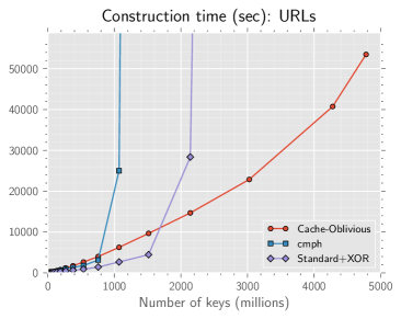
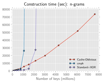
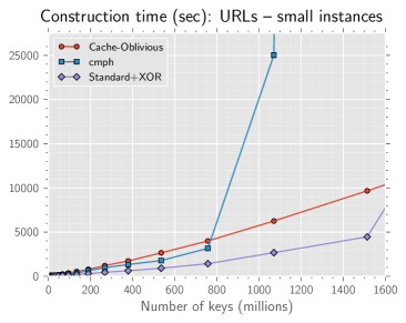
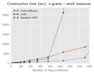
Figure 1: Above: construction times on the two datasets. Below: close-up for $n$ up to $1.6\cdot 10^{9}$ keys.

We can also see that the XOR trick pays off, as shown by the performance of Standard+XOR, which is up to $3$ times faster than cmph, and the smaller space usage enables to process up to almost twice the number of keys for the given memory budget. Both non-external algorithms, though, cease to be useful as soon as the available memory gets exhausted: the machine, then, starts to thrash because of the random patterns of access to the swap. In fact, we had to kill the processes after $48$ hours. Actually, one can make a quite precise estimate of when this is going to happen: cpmh occupies $34.62$ bytes/key, as estimated by the authors, whereas Standard+XOR occupies about $26.76$ bytes/key, and these figures almost exactly justify the two points where the construction times slow down and then explode. On the other hand, Cache-Oblivious scales well with the input size, exhibiting eventually almost linear performance in our larger input ngrams, while remaining competitive even on small key sets.

Comparison with HEM Finally, we compare our algorithm with HEM [6]. Recall that their technique consists in splitting the set of keys into several buckets and building a separate MPHF for every bucket; at query time, a first-level index is used to drive the query to the correct bucket. Choosing a sufficiently small size for the buckets allows the use of a standard internal memory algorithm to construct the bucket MPHF. Although technically not a peeling algorithm, this external-memory solution is simple and elegant.

To make a fair comparison, we re-implemented the HEM algorithm using our sort implementation for the initial bucketing, and the Standard+XOR algorithm to build the bucket MPHFs. The signature function is the same 96-bit hash function used in [6] (which suffice for sets of up to $2^{48}$ keys), but we employed $64$-bit bucket offsets in place of $32$-bit, since our key sets are larger than $2^{32}/\gamma$.

The result, as shown in Figure 2, is a construction time between $2$ and $6$ times smaller than Cache-Oblivious. However, this efficiency has a cost in term of lookup time (because of the double indirection) and size (because of the extra space needed for the first-level index). Since, in most applications, MPHFs are built rarely and queried frequently, the shorter construction time may not be worth the increase in space and query time.

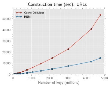
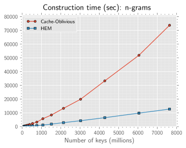
Figure 2: Construction time with the Cache-Oblivious algorithm and HEM [6].

Indeed, as shown in Table 1, the space loss is $17\%$ to $27\%$. The variability in space overhead is due to the fact that in HEM the number of buckets must be a power of $2$, hence the actual average bucket size can vary by a factor of $2$ depending on the number of keys. We also include the space taken by cmph on the largest inputs we were able to construct in-memory. Despite using the same data structure as our implementation of MWHC, its space occupancy is slightly larger because it uses denser ranking tables.

	URLs		ngrams
	$0.76\cdot 10^{9}$ keys	$4.8\cdot 10^{9}$ keys	$0.76\cdot 10^{9}$ keys	$7.6\cdot 10^{9}$ keys
MWHC	2.61 b/key	2.61 b/key	2.61 b/key	2.61 b/key
HEM	3.16 b/key	3.31 b/key	3.16 b/key	3.05 b/key
cmph	2.77 b/key	-	2.77 b/key	-

Table 1: Space comparison of MWCH, HEM, and cmph.

The evaluation of lookup efficiency is much subtler, as it depends on a number of factors, some of which are subject to hardware architecture. For this reason, we decided to perform the experiments on three different machines: an Intel Intel i7-4770 (Haswell) at 3.40GHz, the same Intel i7 (Nehalem) machine used for the construction experiments (see above), and an AMD Opteron 6276 at 2.3GHz.

For both machines and both datasets we performed lookups of $10$ M distinct keys, repeated $10$ times. Since lookup times are in the order of less than a microsecond, it is impossible to measure individual lookups accurately; for this reason, we divided the lookups into $1,\!525$ batches of $2^{16}$ keys each, and measured the average lookup time for each batch. Out of these average times, we computed the global average and the standard deviation. The results in Table 2 show that HEM is slower than MWHC in all cases. On AMD Opteron the slowdown is the smallest, ranging from $17\%$ to $20\%$; on the Intel i7 (Nehalem) the range goes up to $19\%$–$26\%$; on the Intel i7 (Haswell), the most recent and fastest CPU, the slowdown goes up to $30\%$–$35\%$, suggesting that as the speed of the CPU increases, the cost of the causal cache miss caused by the double indirection of HEM becomes more substantial. In all cases, the standard deviation is negligibly small, making the comparison statistically significant.

We also remark that our implementation of the MWHC lookup (which is used also in HEM) is roughly twice as fast than cmph despite using a sparser ranking table; this is because to perform the ranking we adopt a broadword [19] algorithm that counts the number of non-zero pairs in a $64$-bit words in just a few non-branching instructions, rather than a linear bit scan with a loop; the smaller ranking table also imposes a lower cache pressure. Finally, we use a $64$-bit implementation of the Jenkins hash function, which is faster on long strings than the $32$-bit one used in cmph.

	URLs		ngrams
	$0.76\cdot 10^{9}$ keys	$4.8\cdot 10^{9}$ keys	$0.76\cdot 10^{9}$ keys	$7.6\cdot 10^{9}$ keys
	Intel i7 (Haswell)
MWHC	219 ns $\pm$ 0.3%	253 ns $\pm$ 1.3%	199 ns $\pm$ 0.2%	251 ns $\pm$ 1.8%
HEM	284 ns $\pm$ 0.3%	335 ns $\pm$ 1.1%	262 ns $\pm$ 0.3%	338 ns $\pm$ 0.9%
cmph	466 ns $\pm$ 0.3%	-	303 ns $\pm$ 0.3%	-
	Intel i7 (Nehalem)
MWHC	365 ns $\pm$ 0.1%	433 ns $\pm$ 0.1%	334 ns $\pm$ 0.1%	422 ns $\pm$ 0.2%
HEM	450 ns $\pm$ 0.1%	523 ns $\pm$ 0.1%	420 ns $\pm$ 0.1%	502 ns $\pm$ 0.7%
cmph	799 ns $\pm$ 0.1%	-	532 ns $\pm$ 0.1%	-
	AMD Opteron
MWHC	415 ns $\pm$ 0.1%	419 ns $\pm$ 0.1%	373 ns $\pm$ 0.1%	386 ns $\pm$ 0.1%
HEM	484 ns $\pm$ 0.1%	493 ns $\pm$ 0.1%	442 ns $\pm$ 0.2%	463 ns $\pm$ 0.1%
cmph	908 ns $\pm$ 0.2%	-	578 ns $\pm$ 0.3%	-

Table 2: Lookup-time comparison (with relative standard deviation) of MWCH, HEM, and cmph.

References

- [1] Djamal Belazzougui, Paolo Boldi, Rasmus Pagh, and Sebastiano Vigna. Monotone minimal perfect hashing: Searching a sorted table with accesses. In SODA, pages 785–794, 2009.
- [2] Djamal Belazzougui, Paolo Boldi, Rasmus Pagh, and Sebastiano Vigna. Fast prefix search in little space, with applications. In ESA (1), pages 427–438, 2010.
- [3] Djamal Belazzougui, Paolo Boldi, Rasmus Pagh, and Sebastiano Vigna. Theory and practice of monotone minimal perfect hashing. ACM Journal of Experimental Algorithmics, 16, 2011.
- [4] Djamal Belazzougui and Gonzalo Navarro. Alphabet-independent compressed text indexing. In ESA (1), pages 748–759, 2011.
- [5] Djamal Belazzougui and Rossano Venturini. Compressed static functions with applications. In SODA, pages 229–240, 2013.
- [6] Fabiano C. Botelho, Rasmus Pagh, and Nivio Ziviani. Practical perfect hashing in nearly optimal space. Inf. Syst., 38(1):108–131, 2013.
- [7] Fabiano C. Botelho, Nicholas Wormald, and Nivio Ziviani. Cores of random r-partite hypergraphs. Information Processing Letters, 112(8–9):314 – 319, 2012.
- [8] Gerth Stølting Brodal and Rolf Fagerberg. On the limits of cache-obliviousness. In STOC, pages 307–315, 2003.
- [9] Denis Charles and Kumar Chellapilla. Bloomier filters: A second look. In ESA, pages 259–270, 2008.
- [10] Bernard Chazelle, Joe Kilian, Ronitt Rubinfeld, and Ayellet Tal. The Bloomier filter: an efficient data structure for static support lookup tables. In SODA, pages 30–39, 2004.
- [11] Zbigniew J. Czech, George Havas, and Bohdan S. Majewski. Perfect hashing. Theor. Comput. Sci., 182(1-2):1–143, 1997.
- [12] Martin Dietzfelbinger, Andreas Goerdt, Michael Mitzenmacher, Andrea Montanari, Rasmus Pagh, and Michael Rink. Tight thresholds for cuckoo hashing via xorsat. In ICALP (1), pages 213–225, 2010.
- [13] Peter Elias. Universal codeword sets and representations of the integers. IEEE Transactions on Information Theory, 21(2):194–203, 1975.
- [14] Matteo Frigo, Charles E. Leiserson, Harald Prokop, and Sridhar Ramachandran. Cache-oblivious algorithms. ACM Transactions on Algorithms, 8(1):4, 2012.
- [15] Michael T. Goodrich and Michael Mitzenmacher. Invertible Bloom lookup tables. In CCC, pages 792–799, 2011.
- [16] Torben Hagerup and Torsten Tholey. Efficient minimal perfect hashing in nearly minimal space. In STACS, pages 317–326. 2001.
- [17] G. Jacobson. Space-efficient static trees and graphs. In FOCS, pages 549–554, 1989.
- [18] Jiayang Jiang, Michael Mitzenmacher, and Justin Thaler. Parallel peeling algorithms. CoRR, abs/1302.7014, 2013.
- [19] Donald E. Knuth. The Art of Computer Programming. Pre-Fascicle 1A. Draft of Section 7.1.3: Bitwise Tricks and Techniques, 2007.
- [20] Michael Luby, Michael Mitzenmacher, Mohammad Amin Shokrollahi, and Daniel A. Spielman. Efficient erasure correcting codes. IEEE Transactions on Information Theory, 47(2):569–584, 2001.
- [21] Bohdan S. Majewski, Nicholas C. Wormald, George Havas, and Zbigniew J. Czech. A family of perfect hashing methods. Comput. J., 39(6):547–554, 1996.
- [22] Kurt Mehlhorn. On the program size of perfect and universal hash functions. In FOCS, pages 170–175, 1982.
- [23] Michael Mitzenmacher and George Varghese. Biff (Bloom filter) codes: Fast error correction for large data sets. In ISIT, pages 483–487, 2012.
- [24] Michael Molloy. The pure literal rule threshold and cores in random hypergraphs. In SODA, pages 672–681, 2004.
- [25] Michael Molloy. Cores in random hypergraphs and Boolean formulas. Random Structures and Algorithms, 27(1):124–135, 2005.