Abstract

We calculate the one-photon loop radiative corrections to the charged pion-pair production process $\pi^{-}\gamma\to\pi^{+}\pi^{-}\pi^{-}$. In the low-energy region this reaction is governed by the chiral pion-pion interaction. The pertinent set of 42 irreducible photon-loop diagrams is calculated by using the package FeynCalc. Electromagnetic counterterms with two independent low-energy constants $\widehat{k}_{1}$ and $\widehat{k}_{2}$ are included in order to remove the ultraviolet divergences generated by the photon-loops. Infrared finiteness of the virtual radiative corrections is achieved by including soft photon radiation below an energy cut-off $\lambda$. The purely electromagnetic interaction of the charged pions mediated by one-photon exchange is also taken into account. The radiative corrections to the total cross section (in the isospin limit) vary between $+10\%$ close to threshold and about $-1\%$ at a center-of-mass energy of $7m_{\pi}$. The largest contribution comes from the simple one-photon exchange. Radiative corrections to the $\pi^{+}\pi^{-}$ and $\pi^{-}\pi^{-}$ mass spectra are studied as well. The Coulomb singularity of the final-state interaction produces a kink in the dipion mass spectra. The virtual radiative corrections to elastic $\pi^{-}\pi^{-}$ scattering are derived additionally.

1 Introduction and summary

The pions ($\pi^{+},\pi^{0},\pi^{-}$) are the Goldstone bosons of spontaneous chiral symmetry breaking in QCD. Their strong interaction dynamics at low energies can therefore be calculated systematically (and accurately) with chiral perturbation theory in the form of a loop expansion based on an effective chiral Lagrangian. The very accurate two-loop predictions [1] for the S-wave $\pi\pi$-scattering lengths, $a_{0}=(0.220\pm 0.005)m_{\pi}^{-1}$ and $a_{2}=(-0.044\pm 0.001)m_{\pi}^{-1}$, have been confirmed experimentally by analyzing the $\pi\pi$ final-state interaction effects occurring in various (rare) charged kaon decay modes [2, 3, 4, 5]. Electromagnetic processes with pions offer further possibilities to test chiral perturbation theory. For example, pion Compton scattering $\pi^{-}\gamma\to\pi^{-}\gamma$ allows one to extract the electric and magnetic polarizabilities ($\alpha_{\pi}$ and $\beta_{\pi}$) of the charged pion. Chiral perturbation theory at two-loop order gives for the dominant pion polarizability difference the firm prediction $\alpha_{\pi}-\beta_{\pi}=(5.7\pm 1.0)\cdot 10^{-4}\,$fm³ [6]. It is however in conflict with the existing experimental results from Serpukhov $\alpha_{\pi}-\beta_{\pi}=(15.6\pm 7.8)\cdot 10^{-4}\,$fm³ [7, 8] and MAMI $\alpha_{\pi}-\beta_{\pi}=(11.6\pm 3.4)\cdot 10^{-4}\,$fm³ [9], which amount to values more than twice as large. In that contradictory situation it is promising that the COMPASS experiment [10] at CERN aims at measuring the pion polarizabilities, $\alpha_{\pi}$ and $\beta_{\pi}$, with high statistics using the Primakoff effect. The scattering of high-energy negative pions in the Coulomb-field of a heavy nucleus (of charge $Z$) gives access to cross sections for $\pi^{-}\gamma$ reactions through the equivalent photon method [11]. The theoretical framework to extract the pion polarizabilities from the measured cross sections for low-energy pion Compton scattering $\pi^{-}\gamma\to\pi^{-}\gamma$ or the primary pion-nucleus bremsstrahlung process $\pi^{-}Z\to\pi^{-}Z\gamma$ has been described (in the one-loop approximation) in refs. [12, 13]. In addition to the strong interaction effects, the QED radiative corrections to real and virtual pion Compton scattering $\pi^{-}\gamma^{(*)}\to\pi^{-}\gamma$ have been calculated in refs. [13, 14]. The relative smallness of the pion-structure effects in low-energy pion Compton scattering [12] makes it necessary to include such higher order electromagnetic corrections.

The COMPASS experiment is set up to detect simultaneously various (multi-particle) hadronic final-states which are produced in the Primakoff scattering of high-energy pions. The cross sections of the $\pi^{-}\gamma\to 3\pi$ reactions in the low-energy region offer new possibilities to test the strong interaction dynamics of the pions as predicted by chiral perturbation theory. In a recent analysis by the COMPASS collaboration [10, 15] the total cross section for the process $\pi^{-}\gamma\to\pi^{+}\pi^{-}\pi^{-}$ has been extracted in the region from threshold up to a $3\pi$-invariant mass of about $5m_{\pi}$, and good agreement with the prediction of chiral perturbation theory has been found. The analysis of the $\pi^{-}\pi^{0}\pi^{0}$-channel is ongoing [10] and the corresponding experimental results are eagerly awaited. On the theoretical side the production amplitudes for $\pi^{-}\gamma\to\pi^{-}\pi^{0}\pi^{0}$ and $\pi^{-}\gamma\to\pi^{+}\pi^{-}\pi^{-}$ have been calculated at one-loop order in chiral perturbation theory [16]. It has been found that the next-to-leading order chiral corrections enhance sizeably (by a factor $1.5-1.8$) the total cross section for neutral pion-pair production $\pi^{-}\gamma\to\pi^{-}\pi^{0}\pi^{0}$, but leave the one for charged pion-pair production $\pi^{-}\gamma\to\pi^{+}\pi^{-}\pi^{-}$ almost unchanged in comparison to the tree approximation. Let us note that these calculations would be implicitly contained in the work by Ecker and Unterdorfer [17], where the processes $\gamma^{*}\to 4\pi$ have been studied in chiral effective field theory. In particular, the chiral resonance theory used in that work offers the possibility to extend the description of the $\pi^{-}\gamma\to 3\pi$ reactions to higher energies.

The QED radiative corrections to neutral pion-pair production $\pi^{-}\gamma\to\pi^{-}\pi^{0}\pi^{0}$ have been computed recently in ref. [18]. This calculation was simplified by the fact that the virtual photon-loops could be represented by a multiplicative correction factor $R\sim\alpha/2\pi$ to the tree-amplitude and the number of contributing diagrams was limited to one dozen. The purpose of the present work is to extend the calculation of QED radiative corrections to the (more complex) charged pion-pair production process $\pi^{-}\gamma\to\pi^{+}\pi^{-}\pi^{-}$. We use the package FeynCalc [19] to evaluate the difficult set of 42 irreducible photon-loop diagrams. Other contributions of the same order in $\alpha$, such as the one-photon exchange and the soft-photon bremsstrahlung, can still be given in concise analytical formulas. As a result we find that the radiative corrections to the total cross section and the dipion mass spectra in the isospin limit are of the magnitude of a few percent. The largest contribution is provided by the simple one-photon exchange, which reaches up to $8\%$ close to threshold. It is however partly compensated by the leading isospin-breaking correction arising from the charged and neutral pion mass difference. The Coulomb singularity of the $\pi^{\pm}\pi^{-}$ final-state interaction causes a kink in the invariant mass spectra.

Let us clarify that the present analysis is not a complete calculation of all effects of order ${\cal O}(e^{2}p^{2})$ in chiral perturbation theory, since only photon-loops are considered but not the electromagnetic effects induced in pion-loops via the charged and neutral pion mass difference. The latter (subleading) isospin-breaking corrections are expected to be of similar size as the “genuine” radiative corrections studied in this work.

2 Charged pion-pair production: T-matrix and cross section

We start out with recalling the kinematical and dynamical description [16] of the charged pion-pair production process: $\pi^{-}(p_{1})+\gamma(k,\epsilon\,)\to\pi^{+}(p_{2})+\pi^{-}(q_{1})+\pi^{-}(q_{2})$. It is advantageous to choose for the transversal real photon the Coulomb-gauge in the center-of-mass frame, which entails the conditions $\epsilon\cdot p_{1}=\epsilon\cdot k=0$. These subsidiary conditions imply that all diagrams for which the photon $\gamma(k,\epsilon\,)$ couples solely to the incoming negative pion $\pi^{-}(p_{1})$ vanish identically. Under this valid specification the T-matrix has the following general form:

$$T_{\rm cm}={2e\over f_{\pi}^{2}}\Big{[}\vec{\epsilon}\cdot\vec{q}_{1}\,A_{1}+\vec{\epsilon}\cdot\vec{q}_{2}\,A_{2}\Big{]}\,,$$ (1)

where $f_{\pi}=92.4$ MeV denotes the pion decay constant and $e$ is the elementary charge. In the above decomposition $A_{1}$ and $A_{2}$ are two (dimensionless) production amplitudes, which depend on five independent (dimensionless) Mandelstam variables $(s,s_{1},s_{2},t_{1},t_{2})$, defined as:

$$s\,m_{\pi}^{2}=(p_{1}+k)^{2}\,, s_{1}m_{\pi}^{2}=(p_{2}+q_{1})^{2}\,,\quad t_{1}m_{\pi}^{2}=(q_{1}-k)^{2}\,,$$ (2)

$$s_{2}m_{\pi}^{2}=(p_{2}+q_{2})^{2}\,,\quad t_{2}m_{\pi}^{2}=(q_{2}-k)^{2}\,.$$

In this adapted notation $\sqrt{s}\,m_{\pi}$ is the total center-of-mass energy of the process, with $m_{\pi}=139.57\,$MeV the charged pion mass. The introduced set of variables is particularly suitable for describing the permutation of the two identical negative pions in the final state, via the interchanges $(s_{1}\leftrightarrow s_{2},\,t_{1}\leftrightarrow t_{2})$. The second amplitude $A_{2}$ introduced in eq. (1) is determined by the crossing relation:

$$A_{2}(s,s_{1},s_{2},t_{1},t_{2})=A_{1}(s,s_{2},s_{1},t_{2},t_{1})\,,$$ (3)

and therefore it is sufficient to specify only the first amplitude $A_{1}(s,s_{1},s_{2},t_{1},t_{2})$.

At low energies the reaction $\pi^{-}\gamma\to\pi^{+}\pi^{-}\pi^{-}$ is governed by the chiral pion-pion interaction at leading order [16]. It is advantageous to parameterize the special-unitary matrix-field $U$ in the chiral Lagrangian ${\cal L}_{\pi\pi}$ through an interpolating pion-field $\vec{\pi}$ in the form $U=\sqrt{1-\vec{\pi}^{\,2}/f_{\pi}^{2}}+i\vec{\tau}\cdot\vec{\pi}/f_{\pi}$. This has the consequence that no $\gamma 4\pi$ and $\gamma\gamma 4\pi$ contact-vertices exist at leading order. The tree amplitude of chiral perturbation theory reads [16]:

$$A_{1}^{(\rm tree)}={2s-2-s_{1}-s_{2}+t_{1}+t_{2}\over 3-s-t_{1}-t_{2}}+{s-s_{1}-s_{2}+t_{2}\over t_{1}-1}\,,$$ (4)

where in each term the numerator stems from the (off-shell) $\pi\pi$-interaction in the isospin limit (proportional to $f_{\pi}^{-2}$) and the denominator from a pion-propagator. The respective tree diagrams are shown in Fig. 1 of ref. [16] and these coincide with the diagrams in Fig. 2 of the present paper when deleting the external self-energy corrections. Note that the prefactor $2e/f_{\pi}^{2}$ in eq. (1) collects all occurring coupling constants.

Applying the flux factor $[2m_{\pi}^{2}(s-1)]^{-1}$ and a symmetry factor $1/2$, the total cross section for the reaction $\pi^{-}\gamma\to\pi^{+}\pi^{-}\pi^{-}$ is obtained by integrating the (polarization-averaged) squared transversal T-matrix over the three-pion phase space:

$$\sigma_{\rm tot}(s)={\alpha\,m_{\pi}^{2}\over 32\pi^{3}f_{\pi}^{4}(s-1)}\int\limits_{z^{2}<1}\!\!\!\!\!\int\!d\omega_{1}d\omega_{2}\int_{-1}^{1}\!dx\int_{0}^{\pi}\!d\phi\,\big{|}\hat{k}\times(\vec{q}_{1}A_{1}+\vec{q}_{2}A_{2})\big{|}^{2}\,.$$ (5)

Here, $\omega_{1}$ and $\omega_{2}$ are the center-of-mass energies of the outgoing negative pions divided by $m_{\pi}$. In terms of the directional cosines $x=\hat{k}\cdot\hat{q}_{1},\,y=\hat{k}\cdot\hat{q}_{2},\,z=\hat{q}_{1}\cdot\hat{q}_{2}$ the squared cross products in eq. (5) take the form:

$$(\hat{k}\times\vec{q}_{1})^{2}=q_{1}^{2}(1-x^{2})\,,\quad(\hat{k}\times\vec{q}_{2})^{2}=q_{2}^{2}(1-y^{2})\,,\quad(\hat{k}\times\vec{q}_{1})\cdot(\hat{k}\times\vec{q}_{2})=q_{1}q_{2}(z-xy)\,,$$ (6)

with $q_{1,2}=\sqrt{\omega_{1,2}^{2}-1}$ the momenta of the outgoing negative pions divided by $m_{\pi}$, and the subsidiary relations:

$$q_{1}q_{2}\,z=\omega_{1}\omega_{2}-\sqrt{s}(\omega_{1}+\omega_{2})+{s+1\over 2}\,,\quad\quad y=xz+\sqrt{(1-x^{2})(1-z^{2})}\cos\phi\,.$$ (7)

The Mandelstam variables $s_{1},\,s_{2},\,t_{1},\,t_{2}$ follow in the center-of-mass frame as:

$$s_{1}=s+1-2\sqrt{s}\,\omega_{2}\,,\quad s_{2}=s+1-2\sqrt{s}\,\omega_{1}\,,$$

$$t_{1}=1+{1-s\over\sqrt{s}}(\omega_{1}-q_{1}x)\,,\quad t_{2}=1+{1-s\over\sqrt{s}}(\omega_{2}-q_{2}y)\,.$$ (8)

The (bounded) integration region in the $\omega_{1}\omega_{2}$ plane is determined by the inequality $z^{2}<1$. It is straightforward to solve at fixed $\omega_{1}$ the quadratic equation for the upper and lower limit $\omega_{2}^{\pm}$ of the $\omega_{2}$-integration:

$$\omega_{2}^{\pm}={1\over 2}\Bigg{(}\sqrt{s}-\omega_{1}\pm q_{1}\,\sqrt{s-2\sqrt{s}\omega_{1}-3\over s-2\sqrt{s}\omega_{1}+1}\,\Bigg{)}\,,\qquad{\rm for}\quad 1<\omega_{1}<{s-3\over 2\sqrt{s}}\,.$$ (9)

The right hand side of eq. (5) allows to calculate also the dipion mass spectra of the process $\pi^{-}\gamma\to\pi^{+}\pi^{-}\pi^{-}$ by omitting one integration over an energy variable.

3 Radiative corrections

In this section we present the radiative corrections of relative order $\alpha=e^{2}/4\pi=1/137.036$ to the charged pion-pair production process $\pi^{-}\gamma\to\pi^{+}\pi^{-}\pi^{-}$. These include the purely electromagnetic interaction of the charged pions mediated by one-photon exchange and the one-photon loop corrections to the tree level diagrams of chiral perturbation theory. Electromagnetic counterterms [20] will be needed in order to eliminate the ultraviolet divergences generated by the virtual photon-loops. Infrared finiteness of the radiative corrections is achieved in the standard way by including soft-photon bremsstrahlung below an energy cutoff.

3.1 One-photon exchange

Figure 1: Representative set of one-photon exchange diagrams for the process $\pi^{-}\gamma\to\pi^{+}\pi^{-}\pi^{-}$. Each diagram has a partner due to the permutation of the two outgoing $\pi^{-}$.

The simplest electromagnetic correction to the process $\pi^{-}\gamma\to\pi^{+}\pi^{-}\pi^{-}$ at low energies is given by describing the $\pi^{-}\pi^{-}$ interaction in terms of the one-photon exchange. A representative subset of the 10 corresponding tree diagrams is shown in Fig. 1. The diagrams (in the upper row) involving the $\pi\pi\gamma\gamma$ contact-vertex of scalar quantum electrodynamics lead to the following production amplitude:

$$A_{1}^{(\gamma\gamma)}=4\pi\alpha\,{f_{\pi}^{2}\over m_{\pi}^{2}}\bigg{\{}{2\over s_{1}}+{1\over s_{2}}+{1\over 2-s+s_{2}-t_{1}}\bigg{\}}\,,$$ (10)

while the additional diagrams with three ordinary $\pi\pi\gamma$ vertices (in the lower row) give rise to the production amplitude:

$$A_{1}^{(\gamma)} = 4\pi\alpha\,{f_{\pi}^{2}\over m_{\pi}^{2}}\Bigg{\{}{1\over 3-s-t_{1}-t_{2}}\bigg{[}{2s+1-s_{1}-2s_{2}+t_{1}\over s-2-s_{1}+t_{2}}+{2s+1-2s_{1}-s_{2}+t_{2}\over s-2-s_{2}+t_{1}}\bigg{]}$$ (11)

$$+{1\over t_{1}-1}\bigg{[}{1-2s+2s_{1}+s_{2}-t_{1}-2t_{2}\over s_{2}}+{s+1-s_{1}-2s_{2}+t_{1}+t_{2}\over s-2-s_{1}+t_{2}}\bigg{]}\Bigg{\}}\,.$$

The prefactor $f_{\pi}^{2}/m_{\pi}^{2}$ is a consequence of the normalization introduced in eq. (1).

3.2 Photon-loop diagrams and electromagnetic counterterms

Figure 2: Representative set of diagrams including wave function renormalization. For each diagram the self-energy correction can also be placed on the other three external legs.

The virtual radiative corrections to $\pi^{-}\gamma\to\pi^{+}\pi^{-}\pi^{-}$ are obtained by dressing the (three) tree diagrams with a photon-loop in all possible ways. It is helpful to divide these loop diagrams into three classes: self-energy corrections on external pion-lines (I), vertex corrections to the pion-photon coupling (II), and “irreducible” photon-loop diagrams (III). We use dimensional regularization to treat both ultraviolet and infrared divergences (where the latter are caused by the masslessness of the photon). Divergent pieces of one-loop integrals show up in the form of the composite constant:

$$\xi={1\over d-4}+{1\over 2}(\gamma_{E}-\ln 4\pi)+\ln{m_{\pi}\over\mu_{r}}\,,$$ (12)

containing a simple pole at $d=4$. The arbitrary mass scale $\mu_{r}$ is introduced in order to keep (via a prefactor $\mu_{r}^{4-d}$) the mass dimension of one-loop integrals independent of $d$. Ultraviolet (UV) and infrared (IR) divergences are distinguished by the feature of whether $d<4$ or $d>4$ is the condition for convergence of the $d$-dimensional integral. We discriminate them in the notation by putting appropriate subscripts, i.e. $\xi_{UV}$ and $\xi_{IR}$. In order to simplify all calculations we employ the Feynman gauge, where the photon propagator is directly proportional to the Minkowski metric tensor $g_{\mu\nu}$.

Fig. 2 shows a representative subset of the 12 photon-loop diagrams with a self-energy correction on an external pion-line. The corresponding production amplitude $A_{1}^{(\rm I)}$ is the tree amplitude in eq. (4) multiplied with twice the (electromagnetic) wave function renormalization factor $Z_{2}^{(\gamma)}-1$ of the charged pion:

$$A_{1}^{(\rm I)}=A_{1}^{(\rm tree)}\,{2\alpha\over\pi}(\xi_{IR}-\xi_{UV})\,.$$ (13)

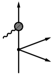
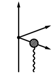
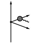
$\vbox{\hbox{\includegraphics[scale={0.8},clip]{blob1.ps}}}\ \Large{=}\ \vbox{\hbox{\includegraphics[scale={0.8},clip]{blob2.ps}}}\ \Large{\bf+}\ \vbox{\hbox{\includegraphics[scale={0.8},clip]{blob3.ps}}}\Large{\bf+}\ \vbox{\hbox{\includegraphics[scale={0.8},clip]{blob4.ps}}}\ \Large{+}\ \vbox{\hbox{\includegraphics[scale={0.8},clip]{blob5.ps}}}$

Figure 3: Diagrams including photonic vertex corrections. In the lower row the incoming pion is off-shell.

Fig. 3 shows (reducible) photon-loop diagrams including vertex corrections to the pion-photon coupling. The blob introduced in the upper row stands for the sum of the four diagrams depicted in the lower row. This whole class of diagrams leads to a vanishing production amplitude:

$$A_{1}^{(\rm II)}=0\,,$$ (14)

where the zero results from the sum:

$$0 = {\alpha\over\pi}\bigg{[}-\xi_{UV}+1-{u+1\over 2u}\ln(1-u)\bigg{]}+{\alpha\over 8\pi}(6\xi_{UV}-7)$$ (15)

$$+{\alpha\over 8\pi}\bigg{[}6\xi_{UV}-6-{1\over u}+{u-1\over u^{2}}(3u+1)\ln(1-u)\bigg{]}$$

$$+{\alpha\over 8\pi}\bigg{[}-4\xi_{UV}+5+{1\over u}+{u^{2}+6u+1\over u^{2}}\ln(1-u)\bigg{]}\,.$$

Here, each of the four summands corresponds to a diagram in the lower row of Fig. 3 (in the order shown) and $u$ abbreviates the variable $(p_{2}-k)^{2}/m_{\pi}^{2}$, $(q_{1}-k)^{2}/m_{\pi}^{2}$, or $(q_{2}-k)^{2}/m_{\pi}^{2}$ depending on which outgoing pion-line the vertex corrections take place. Note that the first term in eq. (15) is the once-subtracted (off-shell) self-energy of the pion. Nevertheless, it is most advantageous to combine it with the (proper) vertex corrections in Fig. 3 in order to obtain the zero-sum. The same pattern of cancellation has been observed in section 2 of ref. [18].

Figure 4: Representative set of irreducible photon-loop diagrams for $\pi^{-}\gamma\to\pi^{+}\pi^{-}\pi^{-}$.

In the remaining loop diagrams the virtual photon connects two charged pions with each other. Fig. 4 shows for a selected pion-pair the 7 diagrams which result from all possible couplings of the incoming photon $\gamma(k,\epsilon\,)$. Given the 6 possible pion-pairs, there are in total $6\cdot 7=42$ such “irreducible” photon-loop diagrams for the process $\pi^{-}\gamma\to\pi^{+}\pi^{-}\pi^{-}$. We have evaluated these diagrams by using the Mathematica package FeynCalc [19]. After reduction to basic scalar loop-functions the corresponding production amplitude $A_{1}$ consists of several hundreds of terms, which prohibits a reproduction of the explicit analytical expression in this paper. A good check of the completeness of diagrams in the automatized calculation is provided by the crossing relation between $A_{2}$ and $A_{1}$ in eq. (3). The irreducible photon-loop diagrams generate also an ultraviolet divergent contribution. We have extracted this piece and after combining it with the $\xi_{UV}$-term from class I written in eq. (13) one gets in total the following ultraviolet divergent contribution from the virtual photon-loops:

$$A_{1}^{(\rm UV-div)}={3\alpha\over 2\pi}\,\xi_{UV}\bigg{[}{2s-s_{1}-s_{2}+t_{1}+t_{2}\over 3-s-t_{1}-t_{2}}+{s+2-s_{1}-s_{2}+t_{2}\over t_{1}-1}\bigg{]}\,.$$ (16)

Note that $A_{1}^{(\rm UV-div)}$ is not proportional to the tree amplitude $A_{1}^{(\rm tree)}$ written in eq. (4). Since chiral perturbation theory with inclusion of virtual photons is a non-renormalizable effective field theory, the cancellation of ultraviolet divergences in radiative corrections requires the consideration of additional electromagnetic counterterms. The complete Lagrangian ${\cal L}_{e^{2}p^{2}}$ of order ${\cal O}(e^{2}p^{2})$ consists of 11 different terms and has been given in eq. (3.6) of ref. [20]. We have extracted from ${\cal L}_{e^{2}p^{2}}$ all those vertices which are relevant for the process $\pi^{-}\gamma\to\pi^{+}\pi^{-}\pi^{-}$ considered here. After evaluation of the tree diagrams shown in Fig. 5 one obtains the following contribution to the production amplitude $A_{1}$ from the electromagnetic counterterms:

$$A_{1}^{(\rm ct)} = {\alpha\over 2\pi}\bigg{\{}(3\xi_{UV}+\widehat{k}_{1})\bigg{[}{s_{1}+s_{2}-2s-t_{1}-t_{2}\over 3-s-t_{1}-t_{2}}+{s_{1}+s_{2}-s-t_{2}-2\over t_{1}-1}\bigg{]}$$ (17)

$$\qquad-\,\widehat{k}_{2}\,\bigg{(}{1\over 3-s-t_{1}-t_{2}}+{1\over t_{1}-1}\bigg{)}\bigg{\}}\,,$$

with the two linear combinations of low-energy constants:

$$\widehat{k}_{1}={16\pi^{2}\over 9}(10k_{1}^{r}-26k_{2}^{r}-54k_{3}^{r}-27k_{4}^{r})-{3\over 2}-3\ln{m_{\pi}\over\mu_{r}}\,,$$ (18)

$$\widehat{k}_{2}={64\pi^{2}\over 9}(18k_{3}^{r}+9k_{4}^{r}-5k_{5}^{r}+31k_{6}^{r}-k_{7}^{r}+36k_{8}^{r})\,.$$ (19)

The last term $-3/2-3\ln(m_{\pi}/\mu_{r})$ in eq.(18) comes from matching our convention for the ultraviolet divergence $\xi_{UV}$ to that of ref. [20]. One sees that in the sum $A_{1}^{(\rm UV-div)}+A_{1}^{(\rm ct)}$ the ultraviolet divergence $\xi_{UV}$ drops out. This exact cancellation serves as a further important check of our calculation. It should be noted that the coefficients $\sigma_{i}$ written in eq. (3.11) of ref. [20] (which determine the divergent part of an individual counterterm) are taken here consistently for $Z=0$, since we do not consider the additional electromagnetic effects induced in pion-loops via the charged and neutral pion mass difference. Actually, in the complete ChPT calculation to order ${\cal O}(e^{2}p^{2})$ the low-energy constant $\widehat{k}_{2}$ in eq. (19) would be split into two pieces where one part is used to express the numerator of the chiral tree-amplitude in terms of the physical neutral pion mass square $m^{2}_{\pi^{0}}$ (see eq. (3.13) in ref. [20]).

Figure 5: Representative set of diagrams with electromagnetic counterterms symbolized by square-box vertices. The photon coupling to the other outgoing pions leads to 14 additional diagrams.

3.3 Soft photon bremsstrahlung

In the next step we have to consider the infrared divergent terms proportional to $\xi_{IR}$ present in eq. (13) and in the production amplitude $A_{1}$ from the irreducible photon-loops. At the level of measurable cross sections these get eliminated by contributions from (undetected) soft-photon bremsstrahlung. In its final effect, soft-photon radiation off the in- or outgoing charged pions multiplies the tree-level differential cross section for $\pi^{-}\gamma\to\pi^{+}\pi^{-}\pi^{-}$ by the correction factor:

$$\delta_{\rm soft} = \alpha\,\mu^{4-d}\!\!\!\int\limits_{|\vec{l}\,|<\lambda}\!\!\!{d^{d-1}l\over(2\pi)^{d-2}\,l_{0}}\bigg{\{}{2p_{1}\cdot q_{1}\over p_{1}\cdot l\,q_{1}\cdot l}+{2p_{2}\cdot q_{1}\over p_{2}\cdot l\,q_{1}\cdot l}+{2p_{1}\cdot q_{2}\over p_{1}\cdot l\,q_{2}\cdot l}+{2p_{2}\cdot q_{2}\over p_{2}\cdot l\,q_{2}\cdot l}$$ (20)

$$-{2p_{1}\cdot p_{2}\over p_{1}\cdot l\,p_{2}\cdot l}-{2q_{1}\cdot q_{2}\over q_{1}\cdot l\,q_{2}\cdot l}-{m_{\pi}^{2}\over(p_{1}\cdot l)^{2}}-{m_{\pi}^{2}\over(p_{2}\cdot l)^{2}}-{m_{\pi}^{2}\over(q_{1}\cdot l)^{2}}-{m_{\pi}^{2}\over(q_{2}\cdot l)^{2}}\bigg{\}}\,,$$

which depends on a small energy cut-off $\lambda$. Working out this momentum space integral by the method of dimensional regularization (with $d>4$) one finds two contributions. The first (universal) contribution includes the infrared divergence $\xi_{IR}$ and it has a logarithmic dependence on the cut-off $\lambda$. The detailed expression for $\delta_{\rm soft}^{(\rm uni)}$ reads:

$$\delta_{\rm soft}^{(\rm uni)} = {4\alpha\over\pi}\bigg{(}\ln{m_{\pi}\over 2\lambda}-\xi_{IR}\bigg{)}\bigg{[}(s_{1}+s_{2}+1-s-t_{1}-t_{2})\,{\bf L}(s_{1}+s_{2}-1-s-t_{1}-t_{2})$$

$$+(2-s_{1})\,{\bf L}(s_{1}-4)+(2-s_{2})\,{\bf L}(s_{2}-4)+(s_{2}-s-t_{1})\,{\bf L}(s+t_{1}-s_{2}-2)$$

$$+(s_{1}-s-t_{2})\,{\bf L}(s+t_{2}-s_{1}-2)+(s+1-s_{1}-s_{2})\,{\bf L}(s-1-s_{1}-s_{2})+1\bigg{]}\,,$$

with the logarithmic function:

$${\bf L}(z)={1\over\sqrt{z(4+z)}}\,\ln{\sqrt{z}+\sqrt{4+z}\over 2}\,.$$ (22)

Here, each of the six terms of the form $(\dots)\,{\bf L}(\dots)$ comes from an interference term in eq. (20) and the $1$ at the end from the sum of last four squares. The second contribution is specific for evaluating the soft-photon correction factor $\delta_{\rm soft}$ in the center-of-mass system and imposing an infrared cut-off, $|\vec{l}\,|<\lambda$, in this reference frame. Its explicit expression reads:

$$\delta_{\rm soft}^{(\rm cm)} = {\alpha\over 2\pi}\Bigg{\{}{s+1\over s-1}\ln s+\sum_{j=1}^{3}{2\omega_{j}\over\sqrt{\omega_{j}^{2}-1}}\,\ln\Big{(}\omega_{j}+\sqrt{\omega_{j}^{2}-1}\,\Big{)}$$ (23)

$$+\sum_{j=1}^{6}\int_{0}^{1}dx\,{V_{j}C_{j}\over D_{j}\sqrt{C_{j}^{2}-4sD_{j}}}\,\ln{C_{j}+\sqrt{C_{j}^{2}-4sD_{j}}\over C_{j}-\sqrt{C_{j}^{2}-4sD_{j}}}\Bigg{\}}\,,$$

with

$$\omega_{1}={s+1-s_{2}\over 2\sqrt{s}}\,,\qquad\omega_{2}={s+1-s_{1}\over 2\sqrt{s}}\,,\qquad\omega_{3}=\sqrt{s}-\omega_{1}-\omega_{2}\,,$$ (24)

the center-of-mass energies of the outgoing pions divided by $m_{\pi}$, and the abbreviations:

$$V_{1}=s+1-s_{1}-s_{2}\,,\qquad C_{1}=s+1-s_{1}+(s_{1}-s_{2})x\,,$$

$$D_{1}=1+x(1-x)(s-1-s_{1}-s_{2})\,,$$ (25)

$$V_{2}=s_{1}+s_{2}+1-s-t_{1}-t_{2}\,,\qquad C_{2}=s+1+(s_{1}+s_{2}-s-3)x\,,$$

$$D_{2}=1+x(1-x)(s_{1}+s_{2}-1-s-t_{1}-t_{2})\,,$$ (26)

$$V_{3}=s_{2}-s-t_{1}\,,\qquad C_{3}=s+1-s_{2}\,x\,,\qquad D_{3}=1+x(1-x)(s+t_{1}-s_{2}-2)\,,$$ (27)

$$V_{4}=2-s_{1}\,,\qquad C_{4}=s+1-s_{2}+(s_{1}+2s_{2}-s-3)x\,,\qquad D_{4}=1+x(1-x)(s_{1}-4)\,,$$ (28)

$$V_{5}=s_{1}-s-t_{2}\,,\qquad C_{5}=s+1-s_{1}\,x\,,\qquad D_{5}=1+x(1-x)(s+t_{2}-s_{1}-2)\,,$$ (29)

$$V_{6}=2-s_{2}\,,\qquad C_{6}=s+1-s_{1}+(2s_{1}+s_{2}-s-3)x\,,\qquad D_{6}=1+x(1-x)(s_{2}-4)\,,$$ (30)

for linear polynomials in the dimensionless Mandelstam variables $(s,s_{1},s_{2},t_{1},t_{2})$.

4 Results and discussion

In this section we present and discuss the numerical results for the radiative corrections to the charged pion-pair production process $\pi^{-}\gamma\to\pi^{+}\pi^{-}\pi^{-}$. We study in detail the radiative corrections to the total cross section $\sigma_{\rm tot}(s)$ and to the $\pi^{+}\pi^{-}$ and $\pi^{-}\pi^{-}$ invariant mass spectra. At the level of the production amplitudes the radiative corrections are given in eq. (5) by the real parts of interference terms between $A_{1,2}^{\rm(tree)}$ and $A_{1,2}^{\rm(rad-cor)}\sim\alpha$. The lengthy expressions generated by FeynCalc have been evaluated numerically with the help of the routine LoopTools [21]. By assigning different values to the parameter $\xi_{IR}$ in the code the exact cancellation of infrared divergences from virtual photon-loops and soft-photon radiation (see eq. (21)) has been verified.

4.1 Radiative corrections to total cross section

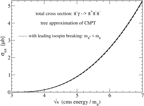
Figure 6: Total cross section $\sigma_{\rm tot}(s)$ of the process $\pi^{-}\gamma\to\pi^{+}\pi^{-}\pi^{-}$ calculated at tree-level in chiral perturbation theory. The full line corresponds to the isospin limit and the dashed line includes the leading isospin-breaking correction due to $m_{\pi^{0}}<m_{\pi}$.

For orientation, we reproduce in Fig. 6 the total cross section $\sigma_{\rm tot}(s)$ of the reaction $\pi^{-}\gamma\to\pi^{+}\pi^{-}\pi^{-}$ calculated at tree-level in chiral perturbation theory [12, 16]. As demonstrated in ref. [16] $\sigma_{\rm tot}(s)$ remains almost unchanged in the region $3<\sqrt{s}<6$ after inclusion of the next-to-leading order chiral corrections (from pion-loops and chiral counterterms in the isospin limit). The dashed line in Fig. 6 is obtained by taking into account the leading isospin-breaking correction due to the difference of the charged and neutral pion mass (see eq. (2.6) in ref. [20]). Isospin-breaking modifies the tree amplitude $A_{1}^{(\rm tree)}$ in such a way that the constant $\delta_{\rm ib}=2(m_{\pi^{0}}/m_{\pi})^{2}-2=-0.1295$ is added to both numerators in eq. (4). The relative correction to the total cross section $\sigma_{\rm tot}(s)$ arising from this effect amounts to $-7.5\%,\,-5.0\%,\,-2.6\%,\,-1.6\%,\,-1.1\%$ at $\sqrt{s}=3.5,\,4,\,5,\,6,\,7$, respectively (see Fig. 8).

Fig. 7 shows in percent the radiative corrections to the total cross section $\sigma_{\rm tot}(s)$ in the region $3<\sqrt{s}<7$. The (lower) dashed-dotted and dashed curves display the effects of the soft-photon bremsstrahlung, separated into the universal contribution proportional to $\ln(m_{\pi}/2\lambda)$ and the contribution specific for imposing the infrared cut-off in the center-of-mass frame. As in refs. [13, 18] the value $\lambda=5\,$MeV has been chosen, which is in the order of magnitude as it appears in the kinematics measured at the COMPASS experiment [22]. The (upper) full line in Fig. 7 shows the effect of the virtual photon-loops. Surprisingly, this radiative correction which requires a huge effort for its computation is almost constant in the region $3.5<\sqrt{s}<7$. With an average value of $1.6\%$ it is also rather close to the analogous result (about $2.2\%$) for neutral pion-pair production $\pi^{-}\gamma\to\pi^{-}\pi^{0}\pi^{0}$ shown in Fig. 5 of ref. [18]. The behavior close to threshold $3<\sqrt{s}<3.5$ is governed by the Coulomb singularity in the $\pi^{\pm}\pi^{-}$ final-state interaction, i.e. the Gamow factor $\pm\pi\alpha/\beta$ with $\beta$ the relative pion velocity [5]. Since the $\pi^{+}\pi^{-}\pi^{-}$ final-state gives rise to two pion-pairs with opposite charges and only one with equal charges the attractive effect (i.e. an enhancement of the cross section) prevails. The effects of the Coulomb singularity will be analyzed in more detail in subsection 4.2 and in the appendix.

Fig. 8 shows by the (upper) dashed line the electromagnetic corrections arising from the one-photon exchange and the sum of the previous contributions (in Fig. 7) is reproduced by the (lower) full curve. With values ranging between $8\pi\alpha f_{\pi}^{2}/m_{\pi}^{2}=8.04\%$ at threshold and $2.1\%$ at $\sqrt{s}=7$ the simple one-photon exchange constitutes the largest correction of relative order $\alpha$. The horizontal grey band shows the additional effects of the electromagnetic counterterms. We have varied the low-energy constants $\widehat{k}_{1}$ and $\widehat{k}_{2}$ in the range $-1\leq\widehat{k}_{1,2}\leq 1$, which is expected to cover electromagnetic counterterms of natural size [20]. Evidently, if one allows for a larger range of the low-energy constants $\widehat{k}_{1,2}$ the band will broaden accordingly. The total sum of the radiative corrections is shown by the dropping band in Fig. 8. The dashed-dotted line is finally obtained by complementing this sum (for $\widehat{k}_{1,2}=0$) by the leading isospin-breaking correction. Putting aside the one-photon exchange contribution which is special for the process $\pi^{-}\gamma\to\pi^{+}\pi^{-}\pi^{-}$, one can conclude that the radiative corrections calculated here are of similar size as in the case of the neutral pion-pair production process $\pi^{-}\gamma\to\pi^{-}\pi^{0}\pi^{0}$ studied in ref. [18]. Moreover, one finds that the one-photon exchange and the leading isospin-breaking correction given by $\delta_{\rm ib}=2(m_{\pi^{0}}/m_{\pi})^{2}-2$ compensate each other partly.

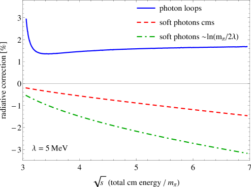
Figure 7: Radiative corrections to the total cross section of the process $\pi^{-}\gamma\to\pi^{+}\pi^{-}\pi^{-}$.

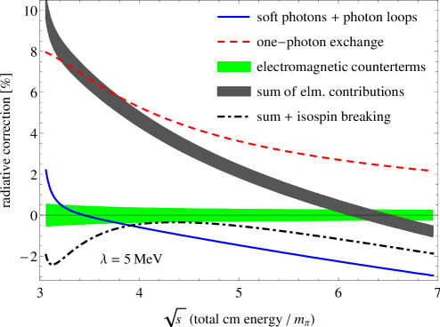
Figure 8: Radiative corrections to the total cross section of the process $\pi^{-}\gamma\to\pi^{+}\pi^{-}\pi^{-}$.

4.2 Radiative corrections to dipion mass spectra

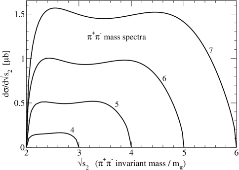
Figure 9: $\pi^{+}\pi^{-}$ mass spectra of the process $\pi^{-}\gamma\to\pi^{+}\pi^{-}\pi^{-}$ as a function of the $\pi^{+}\pi^{-}$ invariant mass $\sqrt{s_{2}}\,m_{\pi}$ for values of $\sqrt{s}=4,5,6,7$.

In this subsection we study the radiative corrections to more exclusive observables of the process $\pi^{-}\gamma\to\pi^{+}\pi^{-}\pi^{-}$, namely the dipion mass spectra. We start with the $\pi^{+}\pi^{-}$ mass spectrum. In terms of the Mandelstam variables the $\pi^{+}\pi^{-}$ invariant mass is $\sqrt{s_{2}}\,m_{\pi}$. Exploiting the relation $s_{2}=s+1-2\sqrt{s}\omega_{1}$, one sees that the differential cross section $d\sigma/d\sqrt{s_{2}}$ is obtained from the right hand side of eq. (5) by leaving out the integration over $\omega_{1}$ and multiplying with a factor $\sqrt{s_{2}/s}$. Again for orientation, we reproduce in Fig. 9 the $\pi^{+}\pi^{-}$ mass spectrum calculated at tree-level in the isospin limit [16]. The numbers next to the curves are the values of $\sqrt{s}$. The radiative corrections arising from soft-photon bremsstrahlung and virtual photon-loops are shown by the dashed and solid curves in Fig. 10. Note that these corrections are given here in absolute units of microbarn, without dividing by the respective mass spectra at tree-level. The pattern of radiative corrections is completed in Fig. 11, where the effect the one-photon exchange and the sum of all contributions are shown. Throughout, one observes positive corrections to $d\sigma/d\sqrt{s_{2}}$ from the virtual photon-loops and the one-photon exchange and negative corrections from the soft-photon radiation. In the total sum of all contributions oscillations and sign-changes occur, which get more pronounced with increasing $\sqrt{s}$. The overlying bands produced by the variation of the low-energy constants $\widehat{k}_{1}$ and $\widehat{k}_{2}$ have not been included for reasons of a cleaner presentation.

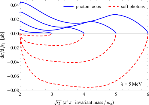
Figure 10: Radiative corrections to the $\pi^{+}\pi^{-}$ mass spectrum of the process $\pi^{-}\gamma\to\pi^{+}\pi^{-}\pi^{-}$ for $\sqrt{s}=4,5,6,7$.

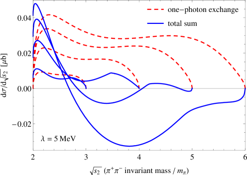
Figure 11: Radiative corrections to the $\pi^{+}\pi^{-}$ mass spectrum of the process $\pi^{-}\gamma\to\pi^{+}\pi^{-}\pi^{-}$ for $\sqrt{s}=4,5,6,7$.

A striking feature visible in Figs. 10, 11 is that the full curves are not smooth, but have kinks at intermediate values of $\sqrt{s_{2}}$. These kinks are by no means numerical artifacts, but they have a clear physical origin in the Coulomb singularity of the electromagnetic $\pi^{\pm}\pi^{-}$ final-state interaction. Let us elaborate on this close relationship in more detail. At fixed $s_{2}$ the range of the (integration) variable $s_{1}$ is $s_{1}^{-}<s_{1}<s_{1}^{+}$ with:

$$s_{1}^{\pm}={1\over 2}\Bigg{(}3+s-s_{2}\pm\sqrt{s_{2}-4\over s_{2}}\,\sqrt{(s+1-s_{2})^{2}-4s}\,\Bigg{)}\,,$$ (31)

where $4<s_{2}<(\sqrt{s}-1)^{2}$. The isolated Coulomb singularity $1/\sqrt{s_{1}-4}$ leads to a dipion mass spectrum of the form:

$$F(\sqrt{s_{2}}\,)=\int_{s_{1}^{-}}^{s_{1}^{+}}ds_{1}\,{1\over\sqrt{s_{1}-4}}=2\sqrt{s_{1}^{+}-4}-2\sqrt{s_{1}^{-}-4}\,.$$ (32)

The just constructed function $F(\sqrt{s_{2}}\,)$ is shown by the full lines in Fig. 12 for $\sqrt{s}=4,5,6,7$. One observes a sharp kink at the position $s_{2}=(s-1)/2$, which is determined by the solution of the equation $s_{1}^{-}=4$. At this point the integral in eq. (32) extends fully into the inverse square-root singularity. One finds by a simple calculation that the left and right derivative of $F(\sqrt{s_{2}}\,)$ with respect to the variable $\sqrt{s_{2}}$ at this point are different with values: $\sqrt{2/(s-9)}\big{[}\pm 8-\sqrt{2(s-1)}\,\big{]}$. Therefore, this example demonstrates that the Coulomb singularity causes inevitably a kink in the two-pion mass spectrum. Actually, it is evidence for the accuracy of the employed numerical methods when this kink is visible in the $\pi^{+}\pi^{-}$ mass spectra calculated from a large number of terms. It is also interesting to consider the effects of the resummed Coulomb singularity by evaluating eq. (32) with the integrand $\mp(1-G)/\pi\alpha$, where $G=\eta/(e^{\eta}-1)$ is the Gamow function [5] with $\eta=\mp 2\pi\alpha/\sqrt{s_{1}-4}$. In this treatment the dashed and dashed-dotted curves in Fig. 12 result from the (singular part of the) Coulomb interaction between two pions with opposite and equal charges, respectively. In order to make the higher order electromagnetic effects better visible the fine-structure constant $\alpha$ has been increased by a factor 10 to $\alpha=1/13.7$. One observes that in the attractive case $(-)$ the kink in the dipion mass spectrum becomes more pronounced whereas in the repulsive case $(+)$ it gets apparently smoothened out.

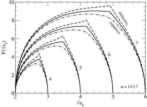
Figure 12: Kink in the dipion mass spectrum at $s_{2}=(s-1)/2$ caused by the Coulomb singularity in the final-state interaction.

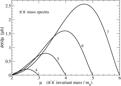
Figure 13: $\pi^{-}\pi^{-}$ mass spectra of the process $\pi^{-}\gamma\to\pi^{+}\pi^{-}\pi^{-}$ as a function of the $\pi^{-}\pi^{-}$ invariant mass $\mu\,m_{\pi}$ for values of $\sqrt{s}=4,5,6,7$.

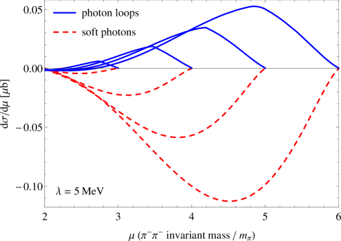
Figure 14: Radiative corrections to the $\pi^{-}\pi^{-}$ mass spectrum of the process $\pi^{-}\gamma\to\pi^{+}\pi^{-}\pi^{-}$ for $\sqrt{s}=4,5,6,7$.

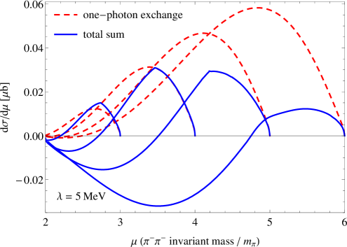
Figure 15: Radiative corrections to the $\pi^{-}\pi^{-}$ mass spectrum of the process $\pi^{-}\gamma\to\pi^{+}\pi^{-}\pi^{-}$ for $\sqrt{s}=4,5,6,7$.

We continue with the discussion of the $\pi^{-}\pi^{-}$ mass spectrum of the process $\pi^{-}\gamma\to\pi^{+}\pi^{-}\pi^{-}$. The $\pi^{-}\pi^{-}$ invariant mass is denoted by $\mu\,m_{\pi}$, where the (dimensionless) variable $\mu$ fulfills the relation $\mu^{2}=s+3-s_{1}-s_{2}=1-s+2\sqrt{s}(\omega_{1}+\omega_{2})$. We introduce the sum $\omega_{+}=\omega_{1}+\omega_{2}$ and half-difference $\omega_{-}=(\omega_{1}-\omega_{2})/2$. After this change of variables, $\omega_{1,2}=\omega_{+}/2\pm\omega_{-}$, the differential cross section $d\sigma/d\mu$ is obtained from the right hand side of eq. (5) by leaving out the integration over $\omega_{+}$ and multiplying with a factor $\mu/\sqrt{s}$. The limits for the remaining integration over $\omega_{-}$ are $\pm\sqrt{\mu^{2}-4}\sqrt{[s-(\mu+1)^{2}][s-(\mu-1)^{2}]}/(4\mu\sqrt{s})$. For the purpose of comparison the $\pi^{-}\pi^{-}$ mass spectra calculated in tree approximation are reproduced in Fig. 13. Note that these have a completely different shape than the $\pi^{+}\pi^{-}$ mass spectra displayed in Fig. 9. The radiative corrections to the differential cross section $d\sigma/d\mu$ as they arise from soft-photon bremsstrahlung, virtual photon-loop and the one-photon exchange are shown in Figs. 14, 15, together with the total sum of these three contributions. The kinks at $\mu=\sqrt{(s-1)/2}$ caused by the Coulomb singularity in the $\pi^{+}\pi^{-}$ final-state interaction appear very prominently in Fig. 15. The overlying bands produced by the variation of the low-energy constants $\widehat{k}_{1}$ and $\widehat{k}_{2}$ have been omitted for reasons of a cleaner presentation.

Altogether, the radiative corrections to the total cross section and dipion mass spectra of the reaction $\pi^{-}\gamma\to\pi^{+}\pi^{-}\pi^{-}$ are of the order of a few percent, with the exception of the region $3<\sqrt{s}<4$ close to threshold. The electromagnetic corrections are indeed below the $5\%$ level as assumed in the analysis of the COMPASS data in ref. [15]. However, with the results of the present work the radiative corrections (as well as the leading isospin-breaking effect) can be consistently taken into account in the analysis of a future high statistics experiment.

Appendix: Virtual radiative corrections to elastic $\pi^{-}\pi^{-}$ scattering

In this appendix we study the virtual radiative corrections to elastic $\pi^{-}\pi^{-}$ scattering. Since $\pi^{-}\pi^{-}\to\pi^{-}\pi^{-}$ is the strong interaction process underlying the charged pion-pair production $\pi^{-}\gamma\to\pi^{+}\pi^{-}\pi^{-}$, it is most instructive to investigate separately the radiative corrections for this simpler subprocess. An essential advantage is that these can be given in closed analytical form. Based on the chiral $\pi\pi$ contact-vertex at leading order, there are 10 associated photon-loop diagrams. For the four diagrams with external self-energy corrections the chiral tree amplitude $T_{-}^{(\rm tree)}=m_{\pi}^{2}(2-s)/f_{\pi}^{2}$ in the isospin limit gets multiplied with twice the (electromagnetic) wave function renormalization factor of the charged pion:

$$T_{-}^{(\rm I)}={2\alpha\,m_{\pi}^{2}\over\pi f_{\pi}^{2}}(2-s)(\xi_{IR}-\xi_{UV})\,.$$ (33)

The two (equal) diagrams with a photon-loop in the $s$-channel (either in the initial or the final state) give together rise to a contribution to the $\pi^{-}\pi^{-}$ scattering amplitude, whose real part reads:

$${\rm Re}\,T_{-}^{(\rm II)} = {\alpha\,m_{\pi}^{2}\over\pi f_{\pi}^{2}}(2-s)\Bigg{\{}4\xi_{UV}-{9\over 2}+{4-s+4(s-2)\xi_{IR}\over\sqrt{s^{2}-4s}}$$ (34)

$$\times\ln{\sqrt{s-4}+\sqrt{s}\over 2}+(2-s)-\int_{4}^{\infty}\!{dx\over x-s}\,{\ln(x-4)\over\sqrt{x^{2}-4x}}\Bigg{\}}\,.$$

Here, we have used the (concise) spectral function representation of the scalar loop integral involving one photon and two pion propagators. In the same way one finds from the two photon-loop diagrams in the $t$-channel:

$$T_{-}^{(\rm III)} = {\alpha\,m_{\pi}^{2}\over\pi f_{\pi}^{2}}\Bigg{\{}\xi_{UV}\bigg{(}s+{3t\over 2}-5\bigg{)}+{13-3s\over 2}-2t+\bigg{[}4st+{3t^{2}\over 2}-8s$$ (35)

$$-10t+16+4(s-2)(2-t)\xi_{IR}\bigg{]}{1\over\sqrt{t^{2}-4t}}\ln{\sqrt{4-t}+\sqrt{-t}\over 2}$$

$$+(s-2)(2-t)\int_{4}^{\infty}\!{dx\over x-t}\,{\ln(x-4)\over\sqrt{x^{2}-4x}}\Bigg{\}}\,,$$

and the contribution from the photon-loops in the $u$-channel is immediately obtained via the substitution $t\to u$:

$$T_{-}^{(\rm IV)} = {\alpha\,m_{\pi}^{2}\over\pi f_{\pi}^{2}}\Bigg{\{}\xi_{UV}\bigg{(}s+{3u\over 2}-5\bigg{)}+{13-3s\over 2}-2u+\bigg{[}4su+{3u^{2}\over 2}-8s$$ (36)

$$-10u+16+4(s-2)(2-u)\xi_{IR}\bigg{]}{1\over\sqrt{u^{2}-4u}}\ln{\sqrt{4-u}+\sqrt{-u}\over 2}$$

$$+(s-2)(2-u)\int_{4}^{\infty}\!{dx\over x-u}\,{\ln(x-4)\over\sqrt{x^{2}-4x}}\Bigg{\}}\,.$$

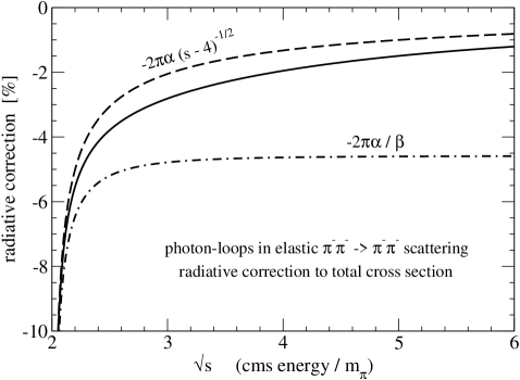
Figure 16: Radiative corrections to the total cross section $\sigma_{\rm tot}(s)$ for elastic $\pi^{-}\pi^{-}$ scattering arising from virtual photon-loops.

Note that we have expressed here the elastic $\pi^{-}\pi^{-}$ scattering amplitude $T_{-}$ in terms of dimensionless Mandelstam variables $(s,t,u)$, which satisfy the constraint $s+t+u=4$ and the inequalities $s>4$ and $t,u<0$ hold in the physical region [1]. The total ultraviolet divergence resulting from the sum of all 10 photon-loop diagrams is: $T_{-}^{(\rm UV-div)}=-(\alpha\,m_{\pi}^{2}/2\pi f_{\pi}^{2})\,3s\,\xi_{UV}$. This piece gets eliminated by the electromagnetic counterterms of ref. [20]. The corresponding contribution to the $\pi^{-}\pi^{-}$ scattering amplitude reads:

$$T_{-}^{(\rm ct)}={\alpha\,m_{\pi}^{2}\over 2\pi f_{\pi}^{2}}\Big{[}(3\xi_{UV}+\widehat{k}_{1})s+\widehat{k}_{2}\Big{]}\,,$$ (37)

with $\widehat{k}_{1}$ and $\widehat{k}_{2}$ the same linear combinations of low-energy constants as written in eqs. (18,19). Let us note that the virtual photon-loops in charged pion-pion scattering have been calculated earlier by Knecht and Nehme [23]. We find perfect agreement with the pertinent terms proportional to $e^{2}$ written in eqs. (12,13) of ref. [23]. The infrared divergence is identified as $\xi_{IR}=\ln(m_{\pi}/m_{\gamma})$ with $m_{\gamma}$ a regulator photon mass. The detailed comparison shows also that the term proportional to the low-energy constant $\widehat{k}_{2}$ in eq. (37) needs to be split up into two pieces and one part has been used in ref. [23] to express the chiral tree amplitude $T_{-}^{(\rm tree)}=[m_{\pi}^{2}(4-s)-2m^{2}_{\pi^{0}}]/f_{\pi}^{2}$ in terms of the physical neutral pion mass.

Of particular interest is the threshold behavior of the last loop-function appearing in eq. (34). By expanding this principal-value integral around $s=4$ for $s>4$ one finds:

$$-\int_{4}^{\infty}\!{dx\over x-s}\,{\ln(x-4)\over\sqrt{x^{2}-4x}}={\pi^{2}\over 2\sqrt{s-4}}-1-{\pi^{2}\over 16}\sqrt{s-4}+{\cal O}(s-4)$$

$$={\pi^{2}\over 4v}(1-v^{2})-1+{\cal O}(v^{2})={\pi^{2}\over 4\beta}(2-\beta^{2})-1+{\cal O}(\beta^{2})\,,$$ (38)

where the first term corresponds to the well-known Coulomb singularity proportional to the inverse pion velocity $v=\sqrt{1-4/s}$ in the center-of-mass frame or the inverse relative velocity $\beta=2v/(1+v^{2})=\sqrt{s(s-4)}/(s-2)$. In non-relativistic quantum mechanics the same electromagnetic initial- or final-state interaction effect is described by the Gamow factor $\pm\pi\alpha/\beta$.

The full line in Fig. 16 shows the radiative corrections to the total cross section $\sigma_{\rm tot}(s)=(64\pi s\,m_{\pi}^{2})^{-1}\int_{-1}^{1}\!dz\,|T_{-}|^{2}$ for elastic $\pi^{-}\pi^{-}$ scattering as they arise from the virtual photon-loops calculated in eqs. (34-36). We have discarded the $\xi_{UV}$ and $\xi_{IR}$ terms which get eliminated by the electromagnetic counterterm and the soft-photon bremsstrahlung. One observes negative corrections of the order of a several percent in the region $2<\sqrt{s}<6$. The behavior close to threshold is governed by the Coulomb singularity $-2\pi\alpha(s-4)^{-1/2}$, which is shown separately by the dashed line in Fig. 16. The dashed-dotted line gives for comparison the (repulsive) Gamow factor $-2\pi\alpha/\beta$ with $\beta=\sqrt{s(s-4)}/(s-2)$ the relative velocity of both pions. One is instructed that the result of the complete calculation in relativistic quantum field theory lies in between these two approximations. Interestingly, the pure Coulomb singularity $-2\pi\alpha(s-4)^{-1/2}$ provides the better approximation. Although the sign and $\sqrt{s}$-dependence are different, the magnitude of these virtual radiative corrections is comparable to the ones shown by the full line in Fig. 7. Note that the one-photon exchange amplitude $T_{-}^{(1\gamma)}=4\pi\alpha[(s-u)t^{-1}+(s-t)u^{-1}]$ for $\pi^{-}\pi^{-}\to\pi^{-}\pi^{-}$ has not been considered here since it would spoil the discussion in terms of the total cross section.

References

- [1] G. Colangelo, J. Gasser, H. Leutwyler, Nucl. Phys. B603, 125 (2001) and references therein.
- [2] S. Pislak et al., Phys. Rev. D67, 072004 (2003).
- [3] J.R. Batley et al., Eur. Phys. J. C54, 411 (2008).
- [4] J.R. Batley et al., Eur. Phys. J. C64, 589 (2009).
- [5] J.R. Batley et al., Eur. Phys. J. C70, 635 (2010).
- [6] J. Gasser, M.A. Ivanov, M.E. Sainio, Nucl. Phys. B745, 84 (2006) and references therein.
- [7] Y.M. Antipov et al., Phys. Lett. B121, 445 (1983).
- [8] Y.M. Antipov et al., Z. Phys. C26, 495 (1985).
- [9] J. Ahrens et al., Eur. Phys. J. A23, 113 (2005).
- [10] S. Paul, J.M. Friedrich, S. Grabmüller, T. Nagel, private communications.
- [11] I.Y. Pomeranchuk, I.M. Shmushkevich, Nucl. Phys. 23, 452 (1961).
- [12] N. Kaiser, J.M. Friedrich, Eur. Phys. J. A36, 181 (2008).
- [13] N. Kaiser, J.M. Friedrich, Nucl. Phys. A812, 186 (2008).
- [14] N. Kaiser, J.M. Friedrich, Eur. Phys. J. A39, 71 (2009).
- [15] COMPASS collaboration: M.G. Alekseev et al., Phys. Rev. Lett. 108, 192001 (2012).
- [16] N. Kaiser, Nucl. Phys. A848, 198 (2010).
- [17] G. Ecker, R. Unterdorfer, Eur. Phys. J. C24, 535 (2002) and references therein.
- [18] N. Kaiser, Eur. Phys. J. A46, 373 (2010).
- [19] R. Mertig, M. Böhm, A. Denner, Comp. Phys. Commun. 64, 345 (1991).
- [20] M. Knecht, R. Urech, Nucl. Phys. B519, 329 (1998) and references therein.
- [21] T. Hahn, M. Perez-Victoria, Comp. Phys. Commun. 118, 153 (1999).
- [22] J.M. Friedrich, ”Chiral Dynamics in Pion-Photon Reactions”, Habilitationsschrift, Technische Universität München (2012), CERN-THESIS-2012-333.
- [23] M. Knecht, A. Nehme, Phys. Lett. B532, 55 (2002).