Bidirectional Recursive Neural Networks
for Token-Level Labeling with Structure
Abstract
Recently, deep architectures, such as recurrent and recursive neural networks have been successfully applied to various natural language processing tasks. Inspired by bidirectional recurrent neural networks which use representations that summarize the past and future around an instance, we propose a novel architecture that aims to capture the structural information around an input, and use it to label instances. We apply our method to the task of opinion expression extraction, where we employ the binary parse tree of a sentence as the structure, and word vector representations as the initial representation of a single token. We conduct preliminary experiments to investigate its performance and compare it to the sequential approach.
1 Introduction
Deep connectionist architectures involve many layers of nonlinear information processing. This allows them to incorporate meaning representations such that each succeeding layer potentially has a more abstract meaning. Recent advancements on efficiently training deep neural networks enabled their application to many problems, including those in natural language processing (NLP). A key advance for application to NLP tasks was the invention of word embeddings that represent a single word as a dense, low-dimensional vector in a meaning space [1], from which numerous problems have benefited [2, 3]. In this work, we are interested in deep learning approaches for NLP sequence tagging tasks in which the goal is to label each token of the given input sentence.
Recurrent neural networks constitute one important class of naturally deep architecture that has been applied to many sequential prediction tasks. In the context of NLP, recurrent neural networks view a sentence as a sequence of tokens. With this view, they have been successfully applied to tasks such as language modeling [4], and spoken language understanding [5]. Since classical recurrent neural networks only incorporate information from the past (i.e. preceding tokens), bidirectional variants have been proposed to incorporate information from both the past and the future (i.e. following tokens) [6]. Bidirectionality is especially useful for NLP tasks, since information provided by the following tokens is usually helpful when making a decision on the current token.
Even though bidirectional recurrent neural networks rely on information from both preceding and following words, capturing long term dependencies might be difficult, due to the vanishing gradient problem [7]: relevant information that is distant from the token under investigation might be lost. On the other hand, depending on the task, a relevant token might be structurally close to the token under investigation, even though it is far away in sequence. As an example, a verb and its corresponding object might be far away in terms of tokens if there are many adjectives before the object, but they would be very close in the parse tree. In addition to a distance-based argument, structure also provides a different way of computing representations: it allows for compositionality, i.e. the meaning of a phrase is determined via a composition of the meanings of the words that comprise it. As a result, we believe that many NLP tasks might benefit from explicitly incorporating the structural information associated with a token.
Recursive neural networks compose another class of architecture, one that operates on structured inputs. They have been applied to parsing [8], sentence-level sentiment analysis [9], and paraphrase detection [10]. Given the structural representation of a sentence, e.g. a parse tree, they recursively generate parent representations in a bottom-up fashion, by combining tokens to produce representations for phrases, eventually producing the whole sentence. The sentence-level representation (or, alternatively, its phrases) is then used to make a final classification for a given input sentence — e.g. whether it conveys a positive or a negative sentiment. Since recursive neural networks generate representations only for the internal nodes in the structured representation, they are not directly applicable to the token-level labeling tasks in which we are interested.
To this end, we propose and explore an architecture that aims to represent the structural information associated with a single token. In particular, we extend the traditional recursive neural network framework so that it not only generates representations for subtrees (i.e. phrases) and the whole sentence upward, but also propagates downward representations toward the leaves, carrying information about the structural environment of each word.
Our method is naturally applicable to any type of labeling task at the word level, however we limit ourselves to an opinion expression extraction task in this work. In addition, although the method is applicable to any type of positional directed acyclic graph structure (e.g. the dependency parse of a sentence), we limit our attention to binary parse trees [8].
2 Preliminaries
2.1 Task description
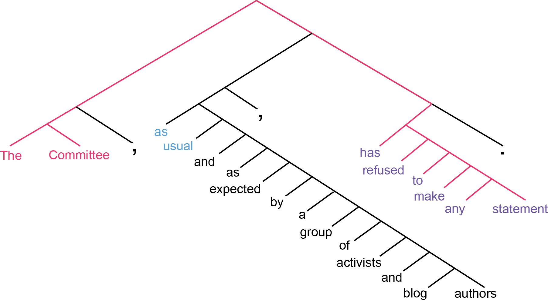
| The | Committee | , | as | usual | , | and | as |
| B_HOLDER | I_HOLDER | O | B_ESE | I_ESE | O | O | O |
| expected | by | a | group | of | activists | and | blog | authors | , |
| O | O | O | O | O | O | O | O | O | O |
| has | refused | to | make | any | statements | . |
| B_DSE | I_DSE | I_DSE | I_DSE | I_DSE | I_DSE | O |
Opinion expression identification aims to detect subjective expressions in a given text, along with their characterizations, such as the intensity and sentiment of an opinion, opinion holder and target, or topic [11]. This is important for tasks that require a fine-grained opinion analysis, such as opinion oriented question answering and opinion summarization. In this work, we focus on the detection of direct subjective expressions (DSEs), expressive subjective expressions (ESEs) and opinion holders and targets, as defined in [11]. DSEs consist of explicit mentions of private states or speech events expressing private states, and ESEs consist of expressions that indicate sentiment, emotion, etc., without explicitly conveying them. An example sentence with the appropriate labels is given in Table 1 in which the DSE “has refused to make any statements” explicitly expresses an opinion HOLDER’s attitude and the ESE “as usual” indirectly expresses the attitude of the writer.
Previously, opinion extraction has been tackled as a sequence labeling problem. This approach views a sentence as a sequence of tokens labeled using the conventional BIO tagging scheme: B indicates the beginning of an opinion-related expression, I is used for tokens inside the opinion expression, and O indicates tokens outside any opinion-related class. Variants of conditional random field-based approaches have been successfully applied with this view [12, 13, 14].
Similar to CRF-based methods, recurrent neural networks can be applied to the problem of opinion expression extraction, with a sequential interpretation. However this approach ignores the structural information that is present in a sentence. Therefore we explore an architecture that incorporates structural information into the final decision.
2.2 Word vector representations
Neural network-based approaches require a vector representation for each input token. In natural language processing, a common way of representing a single token as a vector is to use a “one-hot” vector per token, with a dimensionality of the vocabulary size, such that the corresponding entry of the vector is 1, and all others are 0. This results in a very high dimensional, sparse representation. Alternatively, a distributed representation maps a token to a real valued dense vector of smaller size (usually on the order of 100 dimensions). Generally, these representations are learned in an unsupervised manner from a large corpus, e.g. Wikipedia. Various architectures have been explored to learn these embeddings [1, 2, 15, 16] which might have different generalization capabilities depending on the task [17]. The geometry of the induced word vector space might have interesting semantic properties [16]. In this work, we employ such word vector representations.
2.3 Recurrent neural networks
A recurrent neural network is a class of neural network that has recurrent connections, which allows a form of memory. This makes them applicable for sequential prediction tasks with arbitrary spatio-temporal dimension. This description fits many natural language processing tasks, when a single sentence is viewed as a sequence of tokens. In this work, we focus our attention on only the Elman type networks [18].
In the Elman-type network, the hidden layer at time step is computed from a nonlinear transformation of the current input layer and the previous hidden layer . Then, the final output is computed using the hidden layer . One can interpret as an intermediate representation summarizing the past, which is used to make a final decision on the current input. More formally,
| (1) | ||||
| (2) |
where is a nonlinearity, such as the sigmoid function, is the output nonlinearity, such as the softmax function, and are weight matrices between the input and hidden layer, and among the hidden units themselves (connecting the previous intermediate representation to the current one), respectively, while is the output weight matrix, and and are bias vectors connected to hidden and output units, respectively.
Observe that with this definition, we have information only about the past, when making a decision on . This is limiting for most tasks. A simple way to work around this problem is to include a fixed size future context around a single input vector. However this approach requires tuning the context size, and ignores future information from outside of the context window. Another way to incorporate information about the future is to add bidirectionality to the architecture [6]:
| (3) | ||||
| (4) | ||||
| (5) |
where and are the forward weight matrices as before, and are the backward counterparts of them, , , are the output matrices, and , , are biases. In this setting and can be interpreted as a summary of the past, and the future, respectively, around the time step . When we make a decision on an input vector, we employ both the initial representation and the two intermediate representations and of the past and the future. Therefore in the bidirectional case, we have perfect information about the sequence (ignoring the practical difficulties about capturing long term dependencies, caused by vanishing gradients), whereas the classical Elman type network uses only partial information.
Note that forward and backward parts of the network are independent of each other until the output layer. This means that during training, after backpropagating the error terms from the output layer to the hidden layer, the two parts can be thought as separate, and trained with the classical backpropagation through time [19].
2.4 Recursive neural networks
Recursive neural networks comprise an architecture in which the same set of weights is recursively applied in a structural setting: given a positional directed acyclic graph, it visits the nodes in a topological order, and recursively applies transformations to generate further representations from previously computed representations of children. In fact, a recurrent neural network is simply a recursive neural network with a particular structure. Even though they can be applied to any positional directed acyclic graph, we limit our attention to recursive neural networks over positional binary trees, as in [8].
Given a binary tree structure with leaves having the initial representations, e.g. a parse tree with word vector representations at the leaves, a recursive neural network computes the representations at the internal node as follows:
| (6) |
where and are the left and right children of , an are the weight matrices that connect the left and right children to the parent, and is a bias vector. Given that and are square matrices, and not distinguishing whether and are leaf or internal nodes, this definition has an interesting interpretation: initial representations at the leaves and intermediate representation at the nonterminals lie in the same space. In the parse tree example, recursive neural network combines representations of two subphrases to generate a representation for the larger phrase, in the same meaning space [8]. Depending on the task, we have a final output layer at the root :
| (7) |
where is the output weight matrix and is the bias vector to the output layer. In a supervised task, supervision occurs at this layer. Thus, during learning, initial error is incurred on , backpropagated from the root, towards leaves [20].
3 Methodology
3.1 Bidirectional recursive neural networks
We will extend the aforementioned definition of recursive neural networks, so that it propagates information about the rest of the tree, to every leaf node, through structure. This will allow us to make decisions at the leaf nodes, with a summary of the surrounding structure.
First, we modify the notation in equation (6) so that it represents an upward layer through the tree:
| (8) |
Note that is simply the initial representation if is a leaf, similar to equation (6). Next, we add a downward layer on top of this upward layer:
| (9) |
where is the parent of , and are the weight matrices that connect the downward representations of parent to that of its left and right children, respectively, is the weight matrix that connects the upward representation to the downward representation for any node, and is a bias vector at the downward layer. Intuitively, for any node, contains information about the subtree rooted at , and contains information about the rest of the tree, since every node in the tree has a contributon to the computation of . Therefore and can be thought as complete summaries of the structure around . At the leaves, we use an output layer to make a final decision:
| (10) |
where and are the output weight matrices and is the output bias vector. In a supervised task, supervision occurs at the output layer. Then, during training, error backpropagates upwards, through the downward layer, and then downwards, through the upward layer, employing the backpropagation through structure method [20]. If desired, backpropagated errors can be used to update the initial representation , which allows the possibility of fine tuning the word vector representations, in our setting.
Note that this definition is structurally similar to the unfolding recursive autoencoder [10]. However the goals of the two architectures are different. Unfolding recursive autoencoder downward propagates representations as well. However, the intention is to reconstruct the initial representations. On the other hand, we want the downward representations to be as different as possible than the upward representations , since our aim is to capture the information about the rest of the tree rather than the particular subtree under investigation. Thus, the unfolding recursive autoencoder does not use when computing (except at the root), whereas bidirectional recursive neural network does.
3.2 Incorporating sequential context
Depending on the task, one might want to employ the sequential context around each input vector as well, if the task has the sequential view in addition to structure. To this end, we can combine the bidirectional recurrent neural network with the bidirectional recursive neural network. This allows to use both the sequential information (past and future), and the structural information around a token to produce a final decision:
| (11) |
This architecture can be seen as an extension to both the recurrent and the recursive neural network. During training, after the error term backpropagates through the output layer, individual errors per each of the combined architectures can be handled separately, which allows us to use the previously noted training methods per architecture.
4 Experiments
We cast the problem of detecting DSEs and ESEs as two separate 3-class classification problems. We also experiment with joint detection of DSEs, opinion holders, and opinion target — as a 7-class classification problem with one Outside class and one Beginning and Inside class for DSEs, opinion holders and opinion targets. We compare the bidirectional recurrent neural network as described in Section 2.3 (Bi-Recurrent), the bidirectional recursive network as described in Section 3.1 (Bi-Recursive), and the combined architecture as described in Section 3.2 (Combined). We use the Stanford PCFG parser to extract binary parse trees of sentences [21].
We use precision, recall and F-measure for performance evaluation. Since the boundaries of expressions are hard to define even for human annotators [11], we use two soft notions of the measures: Binary Overlap counts every overlapping match between a predicted and true expression as correct [13, 14], and Proportional Overlap imparts a partial correctness, proportional to the overlapping amount, to each match [22, 14].
We use the manually annotated MPQA corpus [11], which has 14492 sentences in total. For DSE and ESE detection, we separate 4492 sentences as a test set, and run 10-fold cross validation. For joint detection of opinion holder, DSE and target, we have 9471 manually annotated sentences, and we separate 2471 as a test set, and run 10-fold cross validation. A validation set is used to pick the best regularization parameter, simply a coefficient that penalizes the L2 norm.
We use standard stochastic gradient descent, updating weights after minibatches of 80 sentences. We run 200 epochs for training. Furthermore, we fix the learning rate for every architecture, instead of tuning with cross validation, since initial experiments showed that in this setting, every architecture successfully converges without any oscillatory behavior.
As initial representations of tokens, we use pre-trained Collobert-Weston embeddings [2]. Initial experiments with fine tuning the word vector representations presented severe overfitting, hence, we keep the word vectors fixed in the experiments.
We employ the standard softmax activation for the output layer: . For the hidden layers we use the rectifier linear activation: . Experimentally, rectifier activation gives better performance, faster convergence, and sparse representations. Note that in the recursive network, we apply the same transformation to both the leaf nodes and the internal nodes, with the interpretation that they belong in the same meaning space. Employing the rectifier units at the upward layer causes the upward representations at the internal nodes to be always nonnegative and sparse, whereas the initial representations are dense, and might have negative values, which causes a conflict. To test the impact of this, we experimented with the sigmoid activation at the upward layer and the rectifier activation at the downward layer, which caused a degradation in performance. Therefore, at a loss of interpretation, we use the rectifier activation at both layers in our experiments.
The number of hidden layers per architecture is chosen so that every architecture to be compared has the same number of hidden units connected to the output layer as well as the same input dimensionality.
4.1 Results
Experimental results for DSE and ESE detection are given in Tables 2 and 3. For the recurrent network, the topology means that it has input dimensionality , forward hidden layer dimensionality , and backward dimensionality . For the recursive network, means that it has input dimensionality and upward layer dimensionality and a downward layer dimensionality . For the combined network, means an input and upward layer dimensionality , downward layer dimensionality and forward and backward layer dimensionalities and . Asterisk indicates that the performance is statistically significantly better than others in the group, with respect to a two sided paired t-test with .
| Architecture | Topology | Proportional | Binary | ||||
|---|---|---|---|---|---|---|---|
| Prec. | Recall | F1 | Prec. | Recall | F1 | ||
| Bi-Recurrent | (50, 75, 75) | 56.59* | 56.60* | 56.60* | 58.84 | 62.23 | 60.49 |
| Bi-Recursive | (50, 150) | 53.93 | 55.05 | 54.48 | 58.21 | 62.29 | 60.23 |
| Combined | (50, 50, 50, 50) | 54.22 | 53.25 | 53.73 | 58.59 | 62.72 | 60.59 |
| Architecture | Topology | Proportional | Binary | ||||
|---|---|---|---|---|---|---|---|
| Prec. | Recall | F1 | Prec. | Recall | F1 | ||
| Bi-Recurrent | (50, 75, 75) | 45.69 | 53.72 | 49.38 | 52.13 | 65.43 | 58.03 |
| Bi-Recursive | (50, 150) | 42.64 | 53.49 | 47.45 | 47.15 | 71.19* | 56.73 |
| Combined | (50, 50, 50, 50) | 46.16* | 53.33 | 49.49 | 51.95 | 67.49 | 58.71* |
| Architecture | Topology | DSE F1 | Holder F1 | Target F1 | |||
|---|---|---|---|---|---|---|---|
| Prop. | Bin. | Prop. | Bin. | Prop | Bin. | ||
| Bi-Recurrent | (50, 75, 75) | 49.73 | 54.49 | 48.19 | 51.36 | 39.32* | 50.53 |
| Combined | (50, 50, 50, 50) | 50.04 | 54.88 | 49.06* | 52.20* | 38.58 | 49.77 |
We observe that the bidirectional recurrent neural network (Bi-Recurrent) has better performance than both the bidirectional recursive (Bi-Recursive) and the Combined architectures on the task of DSE detection, with respect to the proportional overlap metrics (56.60 F-measure, compared to 54.48, and 53.73). We do not observe a significant difference with respect to the binary overalp metrics. This might be explained by the fact that DSEs tend to be shorter (often even a single word, such as “criticized” or “agrees”). Furthermore, since DSEs exhibit explicit subjectivity, they do not neccessarily require a contextual investigation around the phrase. Most of the time, a DSE can be detected just by looking at the particular phrase.
On the task of ESE detection, the Combined network has significantly better binary F-measure compared to others (58.71 compared to 58.03 and 56.73). Furthermore, the Combined network has significantly better proportional precision than the two other architectures, at an insignificant loss in proportional recall. In terms of binary measures, the Bi-Recursive network has low precision and high recall, which might suggest a complementary behavior for the two architectures. ESEs tend to be longer relative to DSEs, which might explain the results. Aditionally, unlike DSEs, ESEs more often require contextual information for their interpretation. For instance, in the given example in Table 1, it is not clear that “as usual” should be labeled as an ESE, unless one looks at the context presented in the sentence.
Experimental results for joint detection of opinion holder, DSE and target, are given in Table 4 (not to be compared with Table 2, since the datasets are different). Here, the Combined architecture has insignificantly better performance in detecting DSEs (50.04 and 54.88 proportional and binary F-measures, compared to 49.73 and 54.49), and significantly better performance in detecting opinion holders (49.06 and 52.20 proportional and binary F-measures, compared to 48.19 and 51.36), whereas the Bi-Recurrent network is better in detecting targets (39.32 and 50.53 proportional and binary F-measures, compared to 38.58 and 49.77). Again, a possible explanation might be a better utilization of contextual information. To decide whether a named entity is an opinion holder or not, one must link (or fail to link) the entity to an opinion expression. Therefore, it is not possible to decide just by looking at the particular named entity.
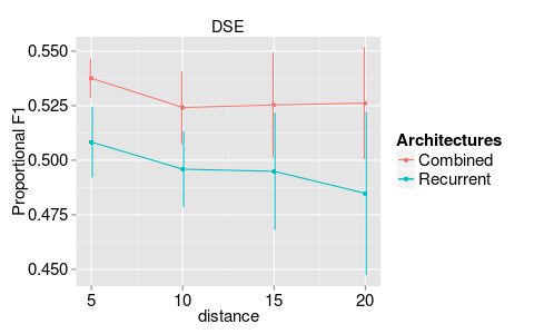
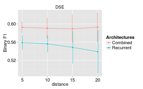
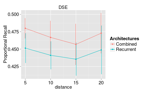
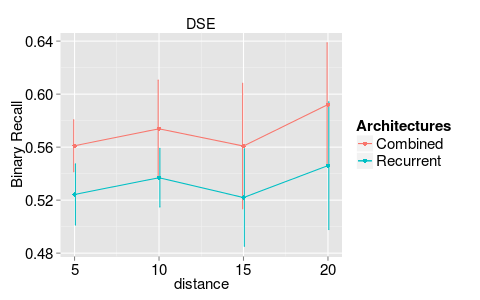
For the joint detection task, we also investigate the performance on a subset of sentences, such that each sentence has at least one DSE and opinion holder, and they are seperated by some distance. This is an attempt to explore the impact of the token-level sequential distance between an opinion holder and an opinion expression. The results are given in Figure 2. As the separation distance increases, on average, DSE detection performance of the combined architecture is steady for the Combined network compared to the Bi-Recurrent network. This might suggest that structural information helps to better capture the cues between opinion holders and expression. Note that each distance-based subset of instances is strictly smaller, since there are fewer number of sentences conforming to the constraints, which causes an increase in variance.
5 Conclusion and Discussion
We have proposed an extension to the recursive neural network to carry out labeling tasks at the token level. We investigated its performance on the opinion expression extraction task. Experiments showed that, depending on the task, employing the structural information around a token might contribute to the performance.
In the bidirectional recursive neural network, downward layer is built on top of the upward layer, whereas in the bidirectional recurrent neural network, forward and backward layers are separate. This causes the supervision to occur at a higher level in the recursive network relative to the recurrent network, which makes training relatively more difficult. To alleviate this difficulty, an unsupervised pre-training of the upward layer, or a similar semi-supervised training, as in [9], might be employed as a future research direction. A fine tuning of the word vector representations during this pre-training might have a positive impact on the performance of the recursive network, since the learned representations for phrases might be structurally more meaningful, compared to the representations learned by sequential, or context window based approaches. Future work will address these observations, investigate more effective training of the bidirectional recursive network and explore the impact of different word vector representations on the architecture.
Acknowledgments
This work was supported in part by DARPA DEFT Grant FA8750-13-2-0015 and a gift from Boeing. The views and conclusions contained herein are those of the authors and should not be interpreted as necessarily representing the official policies or endorsements, either expressed or implied, of DARPA or the U.S. Government.
References
- [1] Yoshua Bengio, Réjean Ducharme, and Pascal Vincent. A neural probabilistic language model. In NIPS, 2001.
- [2] Ronan Collobert and Jason Weston. A unified architecture for natural language processing: Deep neural networks with multitask learning. In Proceedings of the 25th international conference on Machine learning, pages 160–167. ACM, 2008.
- [3] Ronan Collobert, Jason Weston, Léon Bottou, Michael Karlen, Koray Kavukcuoglu, and Pavel Kuksa. Natural language processing (almost) from scratch. J. Mach. Learn. Res., 12:2493–2537, November 2011.
- [4] Tomas Mikolov, Stefan Kombrink, Lukas Burget, JH Cernocky, and Sanjeev Khudanpur. Extensions of recurrent neural network language model. In Acoustics, Speech and Signal Processing (ICASSP), 2011 IEEE International Conference on, pages 5528–5531. IEEE, 2011.
- [5] Grégoire Mesnil, Xiaodong He, Li Deng, and Yoshua Bengio. Investigation of recurrent-neural-network architectures and learning methods for spoken language understanding. In Interspeech, 2013.
- [6] Mike Schuster and Kuldip K Paliwal. Bidirectional recurrent neural networks. Signal Processing, IEEE Transactions on, 45(11):2673–2681, 1997.
- [7] Yoshua Bengio, Patrice Simard, and Paolo Frasconi. Learning long-term dependencies with gradient descent is difficult. Neural Networks, IEEE Transactions on, 5(2):157–166, 1994.
- [8] Richard Socher, Cliff C Lin, Andrew Ng, and Chris Manning. Parsing natural scenes and natural language with recursive neural networks. In Proceedings of the 28th International Conference on Machine Learning (ICML-11), pages 129–136, 2011.
- [9] Richard Socher, Jeffrey Pennington, Eric H Huang, Andrew Y Ng, and Christopher D Manning. Semi-supervised recursive autoencoders for predicting sentiment distributions. In Proceedings of the Conference on Empirical Methods in Natural Language Processing, pages 151–161. Association for Computational Linguistics, 2011.
- [10] Richard Socher, Eric H Huang, Jeffrey Pennin, Christopher D Manning, and Andrew Ng. Dynamic pooling and unfolding recursive autoencoders for paraphrase detection. In Advances in Neural Information Processing Systems, pages 801–809, 2011.
- [11] Janyce Wiebe, Theresa Wilson, and Claire Cardie. Annotating expressions of opinions and emotions in language. Language resources and evaluation, 39(2-3):165–210, 2005.
- [12] Yejin Choi, Claire Cardie, Ellen Riloff, and Siddharth Patwardhan. Identifying sources of opinions with conditional random fields and extraction patterns. In Proceedings of the conference on Human Language Technology and Empirical Methods in Natural Language Processing, pages 355–362. Association for Computational Linguistics, 2005.
- [13] Eric Breck, Yejin Choi, and Claire Cardie. Identifying expressions of opinion in context. In IJCAI, pages 2683–2688, 2007.
- [14] Bishan Yang and Claire Cardie. Extracting opinion expressions with semi-markov conditional random fields. In Proceedings of the 2012 Joint Conference on Empirical Methods in Natural Language Processing and Computational Natural Language Learning, pages 1335–1345. Association for Computational Linguistics, 2012.
- [15] Andriy Mnih and Geoffrey Hinton. Three new graphical models for statistical language modelling. In Proceedings of the 24th international conference on Machine learning, pages 641–648. ACM, 2007.
- [16] Tomas Mikolov, Kai Chen, Greg Corrado, and Jeffrey Dean. Efficient estimation of word representations in vector space. arXiv preprint arXiv:1301.3781, 2013.
- [17] Joseph Turian, Lev Ratinov, and Yoshua Bengio. Word representations: a simple and general method for semi-supervised learning. In Proceedings of the 48th Annual Meeting of the Association for Computational Linguistics, pages 384–394. Association for Computational Linguistics, 2010.
- [18] Jeffrey L Elman. Finding structure in time. Cognitive science, 14(2):179–211, 1990.
- [19] Paul J Werbos. Backpropagation through time: what it does and how to do it. Proceedings of the IEEE, 78(10):1550–1560, 1990.
- [20] Christoph Goller and Andreas Kuchler. Learning task-dependent distributed representations by backpropagation through structure. In Neural Networks, 1996., IEEE International Conference on, volume 1, pages 347–352. IEEE, 1996.
- [21] Dan Klein and Christopher D Manning. Accurate unlexicalized parsing. In Proceedings of the 41st Annual Meeting on Association for Computational Linguistics-Volume 1, pages 423–430. Association for Computational Linguistics, 2003.
- [22] Richard Johansson and Alessandro Moschitti. Syntactic and semantic structure for opinion expression detection. In Proceedings of the Fourteenth Conference on Computational Natural Language Learning, pages 67–76. Association for Computational Linguistics, 2010.