The strength of beta-decays to the continuum

Abstract

The beta-strength in beta-delayed particle decays has up to now been defined in a somewhat ad hoc manner that depends on the decay mechanism. A simple, consistent definition is presented that fulfils the beta strength sum rules. Special consideration is given to the modifications needed when employing R-matrix fits to data. As an example the ¹¹Be($\beta$p) decay is investigated through simple models.

1 Motivation

Close to the beta-stability line all beta-decays will populate particle-bound states, i.e. states that are longlived (stable, beta or gamma decaying) and therefore have narrow widths, less than 1 keV. Moving towards the driplines a larger and larger fraction of beta-decays will feed states that are embedded in the continuum. A general overview of the physics changes this brings about can be found in recent reviews [1, 2]. Close to the dripline beta-delayed particle emission can become the dominating decay mode and the question of how beta strength is assigned to transitions to unbound levels becomes important. This has been discussed at several instances, e.g. [3, 4, 5, 6], the aim of this paper is to provide a consistent answer that is independent of the mechanism for the particle emission. Quite apart from the conceptual interest this also has a very practical implication for the way the total beta strength is calculated: as remarked earlier [5] current approaches give a strength corresponding to decays in an energy region that is proportional to $\int(ft)^{-1}\mathrm{d}E$ for decays going directly to the continuum versus $(\int ft\,\mathrm{d}E)^{-1}$ for decays through a resonance.

To simplify the notation I shall mainly consider Gamow-Teller transitions. For transitions to bound states the decay rate is $w=\ln 2\frac{g_{A}^{2}}{K}f(Q-E)B_{GT}$, where $f$ is the phase space factor, $K=2\ln 2\pi^{3}\hbar^{7}/(m_{e}^{5}c^{4})$ ($m_{e}$ being the electron mass), the beta strength $B_{GT}$ is given by the reduced matrix element squared $|\langle f|\beta_{\pm}|i\rangle|^{2}$ and the weak interaction constant $g_{A}$ is factorized out explicitly from the operator $\beta_{\pm}$ that flips spin and isospin.

The basic suggestion of this paper is to define the beta strength for final unbound states so that the following expression holds for the decay rate:

$$w(E)\mathrm{d}E=\ln 2\frac{g_{A}^{2}}{K}f(Q-E)B_{GT}(E)\mathrm{d}E\;,$$ (1)

where there is an implicit sum over all final states with the same $E$. This definition is in principle experimentally simple to implement, but can be more complex to use theoretically since it does not distinguish between different cases such as isolated resonances in the continuum, interfering resonances, one or several decay channels etc. Essentially one takes out the lepton part ($Q-E$ is the energy going to the beta particle and the neutrino), so it is an attempt to separate the weak interaction part (the “incoming channel”) and the strong interaction part (the “outgoing channel”). A complete separation is not possible unless each decay goes through one and only one intermediate state. As explained in detail later different definitions of $B_{GT}$ have been employed in earlier papers.

Section 2 presents an argument based on the Gamow-Teller sum rule for why the above suggestion is appropriate, and the two following sections compares the definition to existing frameworks. Section 3 looks in detail on beta decays going directly to continuum states and how they have been treated theoretically so far. Section 4 deals with the treatment of decays through intermediate resonances as done in the R-matrix formalism and how this can be modified to be consistent with the proposed definition. Section 5 presents the conclusions and the appendix gives more mathematical details relevant for the R-matrix treatment.

2 Beta strength sum rule

The Gamow-Teller sum-rule is very useful for beta decay studies. It gives a natural scale for $B_{GT}$ for a given decay and is derived by using the completeness relation for rewriting the summed strength for an initial state $|i\rangle$ as

$$S_{\pm}(GT)=\sum_{f}|\langle f|\beta_{\pm}|i\rangle|^{2}=\sum_{f}\langle i|\beta^{\dagger}_{\pm}|f\rangle\langle f|\beta_{\pm}|i\rangle=\langle i|\beta^{\dagger}_{\pm}\beta_{\pm}|i\rangle$$

and by evaluating the commutation relations of the beta operators one gets

$$S_{-}(GT)-S_{+}(GT)=3(N-Z)\;.$$

In this standard derivation of the sum-rule one implicitly assumes a discrete set of final states each with beta strength $B(GT)_{f}=|\langle f|\beta_{\pm}|i\rangle|^{2}$, this must of course be changed when significant contributions come also from continuum states.

A pragmatic way of proceeding that shall be explored later in section 4.1 is to use as a first step a discretized continuum by imposing a finite (but large) quantization volume. By construction the rules for a discrete spectum applies and the sum rule is unchanged. In the continuum limit of increasing quantization volume one would naturally obtain equation (1) and the Gamow-Teller strength will obey the sum rule. Calculations of continuum spectra that proceed by this route will be safe, but other approaches are possible that throw more light on the intricacies of the continuum.

A more formal treatment of the question of how to formulate the completeness relation including continuum states was given by Berggren and collaborators [7, 8]. With a careful definition of the continuum wavefunctions one can derive general sum rules [9, 10] where for our specific case the sum over discrete states is replaced by a sum over bound states and an integral over all (real values of the) momenta in the continuum

$$\sum B_{GT}+\int B_{GT}(k)\mathrm{d}\vec{k}\;.$$ (2)

Berggren further showed how one by allowing complex momenta $k$ and modifying the contour of integration in eq. (2) could extend the sum over bound states to include also contributions from resonance states. Conceptually this gives the crucial insight that even though the physical decay mechanism may favour the description in terms of resonances or the one in terms of continuum transitions we are in principle at liberty to use both (or, in the general case, a mixture). There are two important points to note: first that even when all physical resonances are included in the sum there may remain a small continuum contribution, secondly that in practical implementations one may encounter non-positive contributions from individual terms in the sum as shown explicitly in [11] for the corresponding case of an electric dipole. The resonances that emerge in this framework can therefore not be replaced by or simply identified with the resonances occuring e.g. in the R-matrix framework.

If one in equation (2) integrates $B_{GT}(k)$ over all momenta corresponding to the same energy $E$ one obtains the $B_{GT}(E)$ from above. It is therefore possible to consistently define Gamow-Teller strength in the “pure continuum” so that the sum rule is maintained. If one wishes to assign strength to a specific resonance this can be done, but there is in principle a risk of obtaining non-positive values. The question of when continuum contributions will remain important is treated in [9, 10].

3 Decay directly to continuum

The Berggren approach is being implemented in nuclear structure calculations via the Gamow Shell Model [12], but has so far not been applied to beta-delayed particle emission. Calculations of beta decays directly to a continuum state $|k\rangle$ have been made within several approaches with different conventions for the normalization of continuum states and correspondingly different choices for the normalization of the reduced matrix element $B_{GT}(k)$: in [13] the continuum was discretized in a large volume and the wavefunction normalized to one particle per volume, in other calculations, see e.g. [14, 15, 16], the wavefunctions at large radii become scattering wavefunctions. When calculating the decay rate as a function of the continuum energy $\mathrm{d}w(E)$ one must sum over all states with the same energy $E$. An explicit “phase space factor” for the outgoing particle should therefore be included, a factor that of course also depends on the chosen normalization thereby bringing some confusion to the notation. The conversion to the present definition is for [13]

$$B_{GT}(E)=B_{GT}^{H}(E)\frac{k}{2\pi^{2}}\frac{mc^{2}}{(\hbar c)^{2}}\;,$$

where $k$ and $m$ are the momentum and mass of the outgoing particle. For [14] one has

$$B_{GT}(E)=B_{GT}^{Z}(E)\frac{1}{2\pi^{2}v}\;,$$

where $v$ is the velocity of the outgoing particle. For [16] one has

$$B_{GT}(E)=B_{GT}^{B}(E)\left(\frac{g_{V}}{g_{A}}\right)^{2}\frac{2}{\pi\hbar v}\;,$$

where the extra ratio of coupling constants is due to a different convention that includes them in the definition of $B_{GT}$.

From the previous section it follows that calculations of beta decays going directly to continuum states should essentially automatically fulfil the Gamow-Teller sum rule. The main point in the present definition, equation (1), is for this case only a redefinition of $B_{GT}(E)$ as a sum of all $B_{GT}(k)$ so that the calculation dependent “phase space factor” is not included in the strength definition. This makes comparisons between calculations and between experiment and theory easier.

Up to now the decays that have been described as going directly to continuum states are some of the decay channels of halo nuclei [2]. In the specific case of beta-delayed deuteron decays of two-neutron halo nuclei this is the standard assumption in most theoretical descriptions of the process (based on the picture of the two halo neutrons decaying “remotely” into a deuteron), see e.g. [16] for the most recent calculation of this decay mode in ⁶He. However, a description within the R-matrix approach has also been done [17] and more experimental data may be needed in order to settle whether direct decays is the only reasonable description.

4 Sequential decay

The case of decays through resonances is considerably more complex, in particular for broad resonances where the $f$-factor changes significantly across the level and where interference may play a role. This case is typically analysed with the R-matrix formalism [18, 19] that allows adjusting level parameters to better fit experimental data. Before going into technical details it may be useful to remind why a resonance description is used at all. It is the natural description when there are narrow lines in the experimental spectrum, but it is also of interest more generally since a resonance description summarizes much information into a few numbers. If a few resonances can describe all the structure in a spectrum it gives an economical description that furthermore can be extrapolated (with caution) to neighbouring regions that may be harder to access experimentally.

The R-matrix approach (or an equivalent framework, see [20] for an overview of theoretical approaches that have been used to describe resonance reactions) is essential if there is strong coupling to the continuum or if resonances overlap so that interference occurs, some examples from the light nuclei are the decays of ⁸B, ¹²N, ¹⁷Ne and ¹⁸N. Appendix A contains a more detailed exposition of the R-matrix formalism for beta-delayed decays. I shall mainly consider the single level, singel channel case where, as shown in [6], the decay rate is

$$\mathrm{d}w=\ln 2\frac{g_{A}^{2}}{K}f(Q-E)B_{GT}^{R}\frac{\rho(E)}{\pi}\mathrm{d}E$$

where the size of the beta strength parameter $B_{GT}^{R}$ (essentially the square of the parameter $g$ in [4]) depends explicitly on the normalization of the line shape that is given by

$$\rho_{\lambda}(E)=\frac{P(E)\gamma^{2}_{\lambda}}{[E_{\lambda}-E+(S(E)-B)\gamma^{2}_{\lambda}]^{2}+[P(E)\gamma^{2}_{\lambda}]^{2}}\;.$$ (3)

Here $P,S$ and $B$ are the penetrability, shift function and boundary parameter and $E_{\lambda}$ and $\gamma_{\lambda}$ are the level energy and width parameters. By comparison to the continuum description one sees that $B_{GT}^{R}$ will give the summed beta strength for an isolated level if the integral of $\rho(E)$ is $\pi$. If the integral differs from $\pi$ the basic suggestion of the present paper is that the strength derived from the continuum description is the correct one (it leaves the sum rule unchanged) and is related to the R-matrix parameter $B_{GT}^{R}$ through

$$B_{GT}(E)=B_{GT}^{R}\rho(E)/\pi$$ (4)

so that the integrated strength of the decay through a specific isolated level is $B_{GT}^{R}\int\rho(E)\mathrm{d}E/\pi$.

A very similar correction has been applied by Barker [3, 4, 6], who for narrow levels approximates $\int\rho(E)\mathrm{d}E=\pi/(1+\gamma^{2}_{\lambda}\mathrm{d}S/\mathrm{d}E)$ where the derivative is evaluated at $E_{\lambda}$. This question is analysed in more detail in Appendix A where the limitations of the approximation are exposed. There is no general unique prescription that in a simple manner will give the total beta strength corresponding to a level. Furthermore, if one tries to determine the total strength by performing the integral $\int\rho(E)\mathrm{d}E$, the contribution to the integral above an energy $E_{h}$ will be proportional to $\gamma^{2}_{\lambda}/\sqrt{E_{h}}$ and therefore be potentially large for wide levels. It is not obvious that this contribution at high energies is physically relevant and therefore not obvious which upper integration limit should be used. The best one can do is to employ equation (4) and e.g. determine the strength for decays through a specific level in a given energy range.

The extension from the single-channel, single-level case to the more general situation will not give qualitative changes in the picture. Numerically, the interference that enters in the multi-level case redistributes the beta strength rather than changing its total value. (It seems also to diminish the dependence on $E_{h}$ mentioned above.) In any case, if interference effects are large the whole procedure of attributing beta strength to each individual level may be questioned. The beta strength to a given level cannot be extracted immediately from a spectrum. If one in such cases choses to quote a $B_{GT}$ (or, equivalently, an $ft$-value) the price to pay is that the sum rule is no longer valid and that an evaluation of total strength directly from the spectrum will give a different result (that fullfils the sum-rule).

A pragmatic way to extract beta strength when fitting with the R-matrix formalism is the following: if the resonances are narrow and isolated one can normally use the same procedure as for bound states, except when the variation of the $f$-factor across the level is substantial. In the latter, and other more complex cases, one can either switch to using eq. (1) or equivalently use equation (4) and calculate explicitly the integral of $\rho(E)$ or the corresponding integrals for the multi-channel, multi-level cases given in [4]. Barker uses the Q-value as the upper limit for the integration range (this would correspond to including only the observed strength within the energetically available window), but if the choice has any effect it must be carefully stated.

4.1 A model case: ¹¹Be($\beta$p)

The general results will now be exemplified via a simple tractable case, namely the beta-delayed proton emission from ¹¹Be. This decay mode should be similar to the beta-delayed deuteron decays from two-neutron halo nuclei mentioned above, but is conceptually simpler. A recent paper [21] contains more details on this decay with references to the literature. The model considered here is too simple to be applied immediately to the decay and e.g. does not consider isospin nor decays of core nucleons. Nevertheless, it will serve as a useful illustration.

The basic assumption in this discretized continuum direct decay model (DCDD) is that the initial state is an s-wave neutron in the potential given by ¹⁰Be that is assumed to be inert. The final states are continuum wave functions of a proton in an s-wave in the combined Coulomb and nuclear potential from ¹⁰Be. The Gamow-Teller operator simply converts the halo neutron into a proton (the spin operator will not change the physics) so the matrix element reduces to the overlap between the two wavefunctions. Fermi transitions are assumed to go mainly to the isobaric analogue state and are therefore not included. The final wavefunctions are found as the discrete set of positive energy solutions in a finite volume. The “energy resolution” given by the differences in level energies decrease as the radius of the quantization volume is increased; in the calculations the radius of the volume varied between 400 fm and 4000 fm.

The strong potential between the core and the nucleons is taken as a square well of radius 4.0 fm. This gives an appropriate halo wavefunction for the ¹¹Be ground state when using wavefunctions with one node inside the potential (if wavefunctions with no node are used, the potential radius should be reduced to 3.5 fm). For the initial state the potential strength is adjusted to 33.819 MeV to fit the known ¹¹Be neutron separation energy [22] of 501.64(25) keV. For the final state a square well is used up to 4 fm and a pure Coulomb potential for radii beyond this. The structure of the solutions depend on the well depth used in the final state. For most values one obtains small overlaps with wavefunctions within the 280.7 keV window open for $\beta$p decay and a featureless spectrum. A very similar result was obtained in the more sophisticated two-body calculations of the decay in [23]. This is the “non-resonant” regime with nothing conspicuous appearing in the calculated decay spectrum.

When the depth of the final square well potential is in the range 33–34 MeV one obtains significantly higher overlaps (in this range the final state wavefunctions have one node inside the potential, significant overlaps are also obtained in limited regions where wavefunctions have no or two nodes inside the potential). The obtained overlaps are shown in figure 1 for a 1000 fm confining radius. One observes a “resonance” inside the small window with a width that becomes smaller for lower resonance positions. This behaviour is in contrast to the one observed if one puts the Coulomb potential to zero in the final state (as if the final nucleons were neutrons) in which case there is a broad maximum in the overlaps. A similar behaviour to the one seen here appears in the calculations of beta-delayed deuteron emission in [24] where the final state spectra generally are broad and almost featureless but display a low energy peak for small ranges of the potential depth.

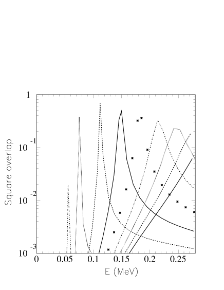
Figure 1: The squared overlap are plotted for each final state wavefunction in the p+¹⁰Be system calculated with a square well of radius 4.0 fm and a confining radius at 1000 fm. The curves are for potential depths (in MeV) of 33.85, 33.8, 33.7, 33.6, 33.5, 33.4, 33.3, 33.2 and 33.1. The initial single-particle wave function is the same for all cases and corresponds to a separation energy of 501.64 keV. All wavefunctions have one node within the potential well.

It may be of interest to briefly compare the found resonances with the famous case of the ⁸Be ground state. Comparing the Schrödinger equations in the tunneling region for the $\alpha+\alpha$ case and for p+¹⁰Be one finds that scaling the radius in the latter case up by the ratio of reduced masses in the two systems and the energies down by the same factor, one obtains exactly the same equation. In other words, the ⁸Be ground state corresponds to a proton resonance at 42 keV. Higher resonance energies correspond to systems more unstable than ⁸Be. In a similar way, when the p+¹⁰Be system is compared to the d+⁹Li one, if the proton radial distances are scaled by a factor 27/20 and the proton energy by a factor 81/80 one obtains exactly the same Schrödinger equation for the two systems in the region below the Coulomb barrier. I.e., the energy scaling factor is here very close to one.

The DCDD model clearly produces a resonance when the effects of the Coulomb barrier are sufficiently strong to confine the wavefunctions. The asymmetry in the line profiles in figure 1 is caused by the decreasing effect of the Coulomb barrier as the energy is raised. An interesting feature can be seen in figure 2 that compares overlaps for three different initial neutron separation energies, 5 keV, 500 keV and 5 MeV. For final state energies around 200 keV the wavefunction gets above the Coulomb barrier at about 29 fm and will start oscillating, i.e. change sign periodically. For the case of 5 keV separation energy the initial wave function will reach out to large distances and the opposite sign contributions are sufficiently strong to give a clearly visible interference dip in the upper tail of the resonance. The finite energy resolution inherent in the direct decay model gives problems for resonance structures at low energy since one cannot be sure to cover the resonance if its width becomes too small and the total overlap from the model becomes prone to numerical uncertainties and therefore unreliable. One can still find the resonance position and width from the procedure outlined in [25], but care must be taken when extracting overlaps.

Figure 2: The squared overlap are plotted for each final state wavefunction in the p+¹⁰Be system calculated with a square well of radius 4.0 fm and depth 33.5 MeV and a confining radius at 4000 fm. The three curves are results for initial single-particle wave functions with different neutron separation energies: 5 keV (solid line), 500 keV (a star for each wavefunction) and 15 MeV (dashed line).

Figure 3: The calculated branching ratio for decay into p+¹⁰Be as a function of resonance position. The stars mark results of DCDD calculations with square well potentials. The filled circles are results from Woods-Saxon potentials when both inital and final wavefunction have one node inside the potential, while the squares correspond to no final state nodes. The dashed curves arise from integrating the R-matrix expression in eq. (6) for assumed alpha-decay widths (in keV) of 0, 0.1, 1, 10 and 100. The full curve is for the expression in eq. (5).

Since all involved states have low energy one would expect the results to be insensitive to the details of the potential shape. This has been tested by performing calculations also with a Woods-Saxon potential with parameters taken from the potential used in [23]. Very similar results were obtained as shown in figure 3 that displays the calculated total branching ratio for beta-delayed proton emission in the two models as a function of the position of the resonance. The $B_{GT}$ was taken as 3, the sum-rule value for a single neutron. To obtain the branching ratio the calculated total decay rate is divided by $w_{tot}=\ln 2/t_{1/2}$. If one has a mismatch between the nodal structure, e.g. one node in the neutron wave function within the potential and no nodes in the final state wave functions, the decay rate decreases as also shown in the figure. (One expects the neutron and proton in the ¹¹Be decay to have the same nodal structure.)

The DCDD model calculations point to a resonance dominated decay, so it is natural to employ also R-matrix calculations of the decay. At first I assume that the level at energy $E_{0}$ fed in beta-decay only decays via proton emission. The expression for the decay rate is then (converted into a differential branching ratio):

$$\frac{\mathrm{d}b}{\mathrm{d}E}=t_{1/2}\frac{g_{A}^{2}}{K}B_{GT}\frac{P\gamma^{2}/\pi}{(E_{0}+\Delta-E)^{2}+(P\gamma^{2})^{2}}f_{\beta}(Q-E)\,,$$ (5)

where $\Delta=-(S(E)-S(E_{0}))\gamma^{2}$ and $P$ and $S$ are the penetrability and shift factors. The value of $\gamma^{2}$ is taken as $\hbar^{2}/(ma^{2})$ which is the maximum possible, the Wigner limit, and where the channel radius used is $a=1.4(1+10^{1/3})$ fm. The $B_{GT}$ is again taken as 3. A simpler approximation sometimes used [5] is to neglect the energy dependence of the shift factor. Doing this and allowing also for $\alpha$-decay from the level gives the following expression:

$$\frac{\mathrm{d}b}{\mathrm{d}E}=t_{1/2}\frac{g_{A}^{2}}{K}B_{GT}\frac{\Gamma_{p}/2\pi}{(E_{0}-E)^{2}+\Gamma_{tot}^{2}/4}f_{\beta}(Q-E)\,,$$ (6)

where $\Gamma_{tot}=\Gamma_{\alpha}+\Gamma_{p}$, the $\alpha$ decay width $\Gamma_{\alpha}$ is assumed to be constant over the Q-window (this should be a good approximation as the $\alpha$ threshold is more than 2.5 MeV lower), $\Gamma_{p}=2P\gamma^{2}$ and $P$ is the standard (energy-dependent) penetrability factor. Integration over the Q-window gives the total branching ratios shown in figure 3 as a function of $E_{0}$ for different values of $\Gamma_{\alpha}$. The branching ratios agree well with the ones from the DCDD model in the region where proton decay dominates, note that the calculation with zero $\Gamma_{\alpha}$ becomes unreliable at very low resonance energies.

Figure 4: The energy spectrum for decays into p+¹⁰Be as a function of centre-of-mass energy. The stars mark results of DCDD calculations with square well potentials. The solid curve are results from an R-matrix calculation employing eq. (5), the dashed curves arise from eq. (6) for assumed alpha-decay widths of 0 keV and 100 keV. See the text for details.

As discussed in detail in Appendix A R-matrix parameters should not be identified immediately with experimentally observed quantities; a correction factor $(1+\gamma^{2}\mathrm{d}S/\mathrm{d}E)^{-1}$ that for our case decreases slightly from 1/2.5 at 50 keV to 1/3 at 200 keV enters often. To illustrate this explicitly figure 4 displays the differential spectra for the DCDD model with potential depth 33.5 MeV and R-matrix calculations from eqs (5) and (6) where in both cases $\gamma^{2}$ is taken as the Wigner limit, $B_{GT}$ is 3 and $E_{0}$ is 181 keV (the approximate resonance position for the DCDD calculation). Comparing first the full R-matrix calculation, eq. (5), with the DCDD results the resonance width and overalll shape are very similar but the overall strength is reduced by the above factor. This explains immediately the corresponding reduction in intensity in figure 3. For the simpler expression from eq. (6) the width is clearly too large, again due to the same correction factor; this underlines that one must insert the observed width (and not the R-matrix width) when using eq. (6). A further effect then enters as the energy dependence of the beta-decay $f$-factor distorts the spectral shape and moves the peak position several keV down. This effect increases with $\Gamma_{tot}$ as also seen in figure 4, a simple evaluation where the energy dependence of the width is neglected and the $f$-factor is approximated as $(Q-E_{0})^{5}$ gives a shift of $-(5/8)\Gamma_{tot}^{2}/(Q-E_{0})$. For the calculation of the total branching ratio a wrong value of the width does not matter as long as the resonance is narrow since the integration over the Breit-Wigner then gives a constant, but it could explain that the results from eq. (6) lie above the other results in figure 3 at energies above 250 keV. When the correct parameter values are inserted in the R-matrix calculations the spectra corresponding to figure 4 agree very well, as do the integrated intensities.

4.2 Implications for R-matrix fits

If fits are made only in a small energy range it does not matter which approximation of R-matrix is used. The larger the energy range, and the larger the effect of having several levels and/or several decay channels, the more obvious is the need to employ the full theory. However, whatever method is used, it is essential to distinguish clearly observed parameters from R-matrix parameters. The main difference in fitting comes from including or neglecting the shift factor (compare eqs (5) and (6)), whereas the energy dependence of the level width $\Gamma=2P(E)\gamma^{2}$ may be inserted or not according to whether its variation is significant. In eq. (6) observed parameters must be inserted (except for the explicit energy variation of the level width), in eq. (5) the R-matrix parameters. The conversion between the two parameter sets is, for narrow levels, via the correction factor $(1+\gamma^{2}\mathrm{d}S/\mathrm{d}E)^{-1}$. For wide levels it eventually becomes meaningless to attempt a conversion. The important fact to note is now that the Wigner limit applies to the R-matrix parameter value, whereas the Gamow-Teller sum rule applies to the observed value. Note further that the “observed $B_{GT}$” only represents the strength present close to the peak. It may be an acceptable value for narrow peaks, but for broader peaks one should apply eq. (4). This holds in particular when interference occurs.

In some cases the observed $B_{GT}$ gives a misleading impression even for narrow levels. This is when the small width $\Gamma=2P\gamma^{2}$ is due to a small penetrability rather than a small value for $\gamma^{2}$ that measures the strength of the coupling to the outgoing channel. In this case one may get a sizable contribution also at higher energies where the penetrability has increased, the “ghost peak” of Barker and Treacy [26]. This effect is also seen in the ¹¹Be($\beta$p) case in the DCDD model for resonance energies below about 65 keV. The effect is mainly due to the change in penetrability, the change in the shape of the final state wave function inside the potential that will be present in the DCDD model is small.

Barker preferred initially [3] to work with ft-values rather than $B_{GT}$ values. There is no conceptual advantage in doing so for broad levels, but it may be slightly simpler experimentally and one does not have to worry about the unfortunate ambiguity in the literature on whether the ratio of coupling constants $(g_{A}/g_{V})^{2}$ is included in $B_{GT}$ or not. For the cases where it is imperative to use R-matrix fits rather than simply treating a resonance as a bound level one has no advantage in using ft-values and the comparison to theory anyway becomes less direct.

Several values of $B_{GT}$ given in the literature will be affected if the present recommendation is followed. The intriguing case of the large asymmetry in the decays of the mirror nuclei ⁹Li and ⁹C will certainly be affected, but the correction factors quoted in [27] are too small to solve the problem. An extreme case with a clear effect is the beta-decay into states in ¹²C above the three-alpha particle threshold. Recent experiments [28, 29] gave a summed strength to identified states up to and including the 12.71 MeV state of 1.0–1.1 for ¹²B and ¹²N. However, further strength is clearly seen at 15–16 MeV excitation energy and if this is interpreted as due to a tail from higher-lying states, as would be naturally assumed from the R-matrix fitting in [29], one would violate the sum rule drastically. If on the other hand the observed strength is summed bin by bin, as done in [28], one obtains a strength of about 0.6 for ¹²N, which is perfectly allowed.

5 Summary

Using the Gamow-Teller sum rule as a guideline this paper puts forward a simple general definition of the beta strength in beta-delayed particle decays. The strength defined in this way differs from the strength entering in the R-matrix formalism, for extreme cases such as the ¹²N decay the difference is large. When beta decays proceed through narrow resonances the expression $B^{R}_{GT}/(1+\gamma^{2}\mathrm{d}S/\mathrm{d}E)$ is a good approximation for the summed strength close to the resonance, but if broad levels are involved or the $Q_{\beta}$-window is large one should use the definition in eq. (1) directly.

The suggested definition also differs quantitatively from the ones employed so far in calculations of decays directly to the continuum, but has the following advantages: (i) the expression for the decay rate, equation (1), is independent of the normalization of the wavefunctions, (ii) the sum over bound states in the sum-rule is extended as

$$\sum B_{GT}+\int B_{GT}(E)\mathrm{d}E$$ (7)

(with the definitions used so far one had to include in the integral an explicit phase space factor) and (iii) the experimental determination of beta strength becomes the same independently of whether the beta decay feeds bound states or the continuum: one simply uses eq. (1) for each bin.

Finally, since most theoretical calculations so far have been carried out in a bound state approximation, any comparison between experiment and theory must be done with great care once the effects treated in this paper are significant.

Acknowledgements I would like to thank D.V. Fedorov, H.O.U. Fynbo, A.S. Jensen, C.A. Diget and S. Hyldegaard for helpful discussions.

Appendix A R-matrix formalism for beta-delayed decays

The basic equations for the case of beta-delayed decays are given by Barker and Warburton [4] and are applicable for several decay channels and several intermediate levels. In their notation the decay rate for channel $c$ is

$$w_{c}(E)=C^{2}f(Q-E)P_{c}(E)|\sum_{\lambda\mu}g_{\lambda,GT}\gamma_{\mu c}A_{\lambda\mu}(E)|^{2}\;,$$ (8)

where the normalization constant $C$ is determined later in their paper, $f$ is the usual beta decay phase space factor, the penetrability (shift factor and boundary parameter) for the channel is $P_{c}$ ($S_{c}$ and $B_{c}$), the levels are indexed by $\lambda$ and $\mu$ with level energy parameter $E_{\lambda}$, coupling parameter $\gamma_{\lambda c}$ to the decay channel $c$ and beta decay parameter to the level $g_{\lambda,GT}$ corresponding to the parameter in the main text $B_{GT}^{R}=g_{\lambda,GT}^{2}$. Finally, the elements of the level matrix are defined through

$$(A^{-1})_{\lambda\mu}(E)=(E_{\lambda}-E)\delta_{\lambda\mu}-\sum_{c}(S_{c}-B_{c}+iP_{c})\gamma_{\lambda c}\gamma_{\mu c}\;.$$ (9)

For a single isolated level and a single decay channel for the levels this expression reduces to the one given just before eq. (3) above. The standard Breit-Wigner expression is obtained by approximating $2P(E_{\lambda})\gamma^{2}_{\lambda}$ by $\Gamma$ and $E_{\lambda}+(S(E_{\lambda})-B)\gamma^{2}_{\lambda}$ by $E_{0}$. Brune [30] has provided an altervative parametrization that avoids boundary parameters and may be more useful in applications.

Barker has argued [3, 4, 6] that the best approximation to the integral of $\rho$ (given in eq. (3)) is

$$\int_{0}^{\infty}\rho_{\lambda}(E)\mathrm{d}E=\frac{\pi}{1+\gamma^{2}_{\lambda}\frac{\mathrm{d}S}{\mathrm{d}E}|_{E_{\lambda}}}$$ (10)

and that the deduced $B_{GT}$ (similar to extracted $\Gamma$-values) must be reduced by dividing with the same denominator. The argument comes from Lane and Thomas [18] and is based on making a first order Taylor expansion of $S(E)=S(E_{\lambda})+(E-E_{\lambda})\mathrm{d}S/\mathrm{d}E$. A standard Breit-Wigner form can then be obtained by pulling out the square of the factor $F=1+\gamma^{2}_{\lambda}\frac{\mathrm{d}S}{\mathrm{d}E}|_{E_{\lambda}}$ from the energy difference in the denominator in eq. (5) so that the effective width, often called observed width, becomes $\Gamma/F$ and similar for the $B_{GT}$ value. Essentially, in this approximation the integral is performed as if the shape in the peak region can be extended trivially to all energies.

A more accurate way of evaluating the total integral is as follows. The expression for $\rho(E)$ can be analytically continued to complex values of the energy $E$ if one places a cut just above the negative real axis, this is needed since the penetrability contains a factor $kR=\sqrt{c^{\prime}E}$. The poles of $\rho_{\lambda}(E)$ appear for

$$E=E_{\lambda}+(S(E)-B)\gamma^{2}_{\lambda}\pm iP(E)\gamma^{2}_{\lambda}$$

and apart from the “classical” pole at $E_{-}=E_{0}-i\Gamma/2$ (and its mirror $E_{+}=E_{0}+i\Gamma/2$) one can have poles from the terms $P(E)$ and $S(E)$. One now extends the integral along the negative real axis and closes it in the lower half so that the residue theorem can be used. The added part in the lower complex plane gives a vanishing contribution and the integral along the negative real axis gives a purely imaginary contribution (except for possible poles on the axis which then have to be evaluated explicitly) due to the factor $\sqrt{E}$, this can be shown explicitly for neutral particles but probably holds in general. The integral can therefore be evaluted simply from the residues at the poles of the function in the lower half where the main contribution (at least for small $\gamma^{2}$) will be from the pole at $E_{-}$. Close to this pole the behaviour is similar to that of the standard Breit-Wigner function but the residue, which for the Breit-Wigner is $2\pi i\Gamma/2/(E_{+}-E_{-})=2\pi i\Gamma/2/(2i\Gamma/2)=\pi$, becomes more complex due to the analytic continuation of $P(E)$ into the complex plane. The correct result for the integral turns out to be $\pi$ also for s-wave neutrons (where $P(E)=kR$ and $S(E)=0$) but for higher angular momenta deviations will occur. One can show in general that each pole $E_{p}$ will give a contribution to the integral of

$$\pi\left(\pm\left[1-\gamma^{2}_{\lambda}\left.\frac{\mathrm{d}S}{\mathrm{d}E}\right|_{E_{p}}\right]\left.-i\gamma^{2}_{\lambda}\frac{\mathrm{d}P}{\mathrm{d}E}\right|_{E_{p}}\right)^{-1}\;,$$

i.e., if the imaginary term can be neglected to lowest order, at first glance a similar result to eq. (10) but with opposite sign! Furthermore, the contributions from the poles that arises from $P(E)$ give a contribution that is of the same order as the correction terms from the classical pole. In fact, an explicit calculation for p-wave neutrons (where $P(E)=(c^{\prime}E)^{3/2}/(1+c^{\prime}E)$ and $S(E)=-1/(1+c^{\prime}E)$) gives to lowest order that the integral is

$$\pi\left(1+2\frac{c^{\prime}\gamma^{2}_{\lambda}}{(1+c^{\prime}E_{\lambda})^{2}}\right)$$

where the classical pole and a pole close to $-1$ contributes equally to the last term. The reason that the Lane and Thomas expansion gives the wrong result is, as pointed out explicitly in [29] for the case of the Hoyle state, that part of the strength appears away from the pole position as so-called ghosts [26]. Whether this contribuiton is physically important or not depends on the specific circumstances of a decay. The summed strength close to the resonance energy will for narrow levels be given to a good approximation by eq. (10).

For the one-level multi-channel case one can see easily from the general formulae in [4] that the only change is to insert a sum over all channels in the terms $(S(E)-B)\gamma^{2}$ and $P(E)\gamma^{2}$. Summing the contribution in all outgoing channels one therefore obtains a result similar to the one-level one-channel case. However, in the multi-level one-channel case interference between the levels will appear. Numerically this does not seem to have a major effect; in fact, for levels that interact constructively between the two peak positions it seems that the total areas are less perturbed than for individual single levels even for cases with rather strong interference (the desctructive interference away from the levels seems to suppress the contributions that makes integrals deviate from $\pi$).

References

- [1] B. Blank and M.J.G. Borge, Prog. Part. Nucl. Phys. 60 (2008) 403
- [2] M. Pfützner, M. Karny, L.V. Grigorenko and K. Riisager, Rev. Mod. Phys. 84 (2012) 567
- [3] F.C. Barker, Aust. J. Phys. 22 (1969) 293
- [4] F.C. Barker and E.K. Warburton, Nucl. Phys. A487 (1988) 269
- [5] G. Nyman et al., Nucl. Phys. A510 (1990) 189
- [6] F.C. Barker, Nucl. Phys. A609 (1996) 38
- [7] T. Berggren, Nucl. Phys. A109 (1968) 265
- [8] T. Berggren and P. Lind, Phys. Rev. C47 (1993) 768
- [9] T. Berggren, Phys. Lett. B44 (1973) 23
- [10] W.J. Romo, Nucl. Phys. A237 (1975) 275
- [11] T. Myo, A. Ohnishi and K. Kato, Prog. Theor. Phys. 99 (1998) 801
- [12] N. Michel, W. Nazarewicz, M. Płoszajczak and T. Vertse, J. Phys. G36 (2009) 013101
- [13] K. Riisager et al., Phys. Lett. 235 (1990) 30
- [14] M.V. Zhukov, B.V. Danilin, L.V. Grigorenko and N.B. Shul’gina, Phys. Rev. C47 (1993) 2937
- [15] D. Baye, Y. Suzuki and P. Descouvemont, Prog. Theor. Phys. 90 (1994) 271
- [16] E.M. Tursunov, D. Baye and P. Descouvemont, Phys. Rev. C73 (2006) 014303
- [17] F.C. Barker, Phys. Lett. B322 (1994) 17
- [18] A.M. Lane and R.G. Thomas, Rev. Mod. Phys. 30 (1958) 257
- [19] P. Descouvemont and D. Baye, Rep. Prog. Phys. 73 (2010) 036301
- [20] D. Robson, in Nuclear Spectroscopy and Reactions, ed. J. Cerny (Academic, New York, 1975), vol. D, p. 179
- [21] M.J.G. Borge et al., J. Phys. G40 (2013) 035109
- [22] M. Wang et al., Chinese Phys. C 36 (2012) 1603
- [23] D. Baye and E.M. Tursonov, Phys. Lett. B696 (2011) 464
- [24] M.V. Zhukov, B.V. Danilin, L.V. Grigorenko and J.S. Vaagen, Phys. Rev. C 52 (1995) 2461
- [25] D.V. Fedorov, A.S. Jensen and M. Thøgersen, Few-Body Syst. 45 (2009) 191
- [26] F.C. Barker and P.B. Treacy, Nucl. Phys. 38 (1962) 33
- [27] Y. Prezado et al., Phys. Lett. B576 55
- [28] S. Hyldegaard et al., Phys. Lett. B678 (2009) 459
- [29] S. Hyldegaard et al., Phys. Rev. C81 (2010) 024303
- [30] C.R. Brune, Phys. Rev. C66 (2002) 044611