Effect of disorder geometry on the critical force in disordered elastic systems

Abstract

We address the effect of disorder geometry on the critical force in disordered elastic systems. We focus on the model system of a long-range elastic line driven in a random landscape. In the collective pinning regime, we compute the critical force perturbatively. Not only our expression for the critical force confirms previous results on its scaling with respect to the microscopic disorder parameters, it also provides its precise dependence on the disorder geometry (represented by the disorder two-point correlation function). Our results are successfully compared to the results of numerical simulations for random field and random bond disorders.

1 Introduction

Disordered elastic systems [1, 2, 3, 4] are ubiquitous in Nature and condensed matter physics; they encompass a wide range of systems going from vortex lattices in superconductors [5] to ferromagnetic domain walls [6], wetting fronts [7], imbibition fronts [8, 9] or crack fronts in brittle solids [10, 11]. In simple models for those phenomena, an elastic object struggles to stay flat while its random environment tries to deform it, in or out of equilibrium. An example is given by an elastic line in a random landscape, that is pictured on Fig. 1. As a result of the competition between disorder and elasticity, the elastic object becomes rough and is characterized by a universal roughness exponent [12, 13] that depends on the dimension of the problem, the range of the elastic interaction and the type of disorder, but not on the microscopic details of the system [2, 4].

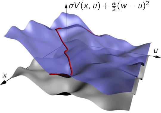
Figure 1: (Colour online) An elastic line pulled by a spring of stiffness $\kappa$ and position $w$ in a random landscape. The bottom grey surface is the potential $\sigma V(x,u)$. The top blue surface is the effective potential seen by the line, i.e. the bare potential plus the parabolic potential $\frac{\kappa}{2}(w-u)^{2}$ exerted to the spring.

This coupling between disorder and elasticity also has an important consequence on the response of the elastic object to an external force [5]. At zero temperature, there exists a critical force below which it does not move and remains pinned by the disorder. If the applied force is larger than this threshold, the elastic object unpins and acquires a non-zero average velocity. This describes the depinning transition of the elastic line. A finite temperature rounds this behaviour for forces close to the threshold [14] and allows the object to move at a finite velocity for forces well below the threshold, by a thermally activated motion called creep [15, 16, 17, 18, 19]. The critical force plays a crucial role in applications. In type-II superconductors, it corresponds to the critical current above which the vortex lattice starts moving, leading to a superconductivity breakdown [20]. In brittle solids, it determines the critical loading needed for a crack to propagate through the sample and break it apart [10].

Contrarily to roughness and depinning exponents, the critical force is not a universal quantity and its value depends in general on the details of the model. However, scaling arguments allow to find its dependence on the disorder amplitude and the different lengthscales present in the system, such as the size of the defects and the typical distance between them [5, 21]. Unfortunately this approach gives the critical force only up to a numerical prefactor, whose value depends on microscopic quantities such as the geometrical shape of the impurities, and which is essential to determine in view of applications. Recently, a numerical self-consistent scheme [22, 23] and numerical simulations have focused on a precise determination of the critical force [24, 25] in the context of brittle failure. Notably, is has been shown that in the collective regime, occurring at weak disorder amplitude, the critical force does not depend on the disorder distribution but only on the disorder amplitude and correlation length [24]. Still, the effect of the disorder geometry, that is partly encoded in its two-point correlation function, remains to be determined.

In this article, we address the question of the dependence of the critical force on the disorder geometry. We focus on the case of a long-range elastic line in a random potential, that is the relevant model for wetting fronts and crack fronts in brittle failure. We restrict ourselves to the collective pinning regime, that appears when the disorder amplitude is small. The line is driven by a spring pulled at constant velocity, and the drag force needed to move the spring is computed perturbatively in the disorder amplitude. In the limit of zero spring stiffness and zero velocity, this force is the critical force and we derive its analytic expression.

Our expression depends explicitly on the two-point correlation function of the disorder, and thus on the disorder geometry. Moreover, our computation is valid for a random bond disorder as well as a random field disorder [18]. Numerical simulations are performed for both types of disorder and various disorder geometries. They provide a successful check of our analytical result and show that two systems with the same disorder amplitude and correlation length can have a different critical force if their two-point correlation functions are different.

The paper is organized as follows. In section 2, we introduce the model of a long-range elastic line driven in a random landscape. In section 3, we summarize our results. Section 4 is devoted to the analytical computation of the drag force, from which we deduce the critical force. Numerical simulations details and results are presented in section 5. We conclude in section 6.

2 Model

We consider a 1+1 dimensional elastic line of internal coordinate $x$ and position $u(x,t)$, pulled by a spring of stiffness $\kappa$ located at position $w(t)$ in a random energy landscape $\sigma V(x,u)$; this system is represented on Fig. 1. The parameter $\sigma$ represents the disorder amplitude. The equation of evolution of the line position at zero temperature is [2, 26]

$$\partial_{t}u(x,t)=\kappa[w(t)-u(x,t)]+f_{\mathrm{el}}[u(\cdot,t)](x)-\sigma\partial_{u}V(x,u(x,t)).$$ (1)

The elastic force $f_{\mathrm{el}}[u(\cdot,t)](x)$ is linear in $u(x,t)$ and we consider the case of a long-range elasticity

$$f_{\mathrm{el}}[u(\cdot,t)](x)=\frac{c}{\pi}\int\frac{u(x^{\prime},t)-u(x,t)}{(x-x^{\prime})^{2}}\mathrm{d}x^{\prime}.$$ (2)

The disorder has zero mean ($\overline{V(x,u)}=0$) and two-point correlation function

$$\overline{V(x,u)V(x^{\prime},u^{\prime})}=R_{x}(x-x^{\prime})R_{u}(u-u^{\prime}).$$ (3)

The overline represents the average over the disorder. Alternatively, one can also use the force correlation function,

$$\overline{\partial_{u}V(x,u)\partial_{u^{\prime}}V(x^{\prime},u^{\prime})} =-R_{x}(x-x^{\prime})\partial_{u}^{2}R_{u}(u-u^{\prime})$$ (4)

$$=\Delta_{x}(x-x^{\prime})\Delta_{u}(u-u^{\prime}).$$ (5)

with $\Delta_{u}=-\partial_{u}^{2}R_{u}$. We do not assume that the disorder is Gaussian distributed. For the so-called random bond (RB) case, the potential $V(x,u)$ is short-range correlated both in the variables $x$ and $u$; this implies a global constraint on the force correlation function, namely $\int\Delta_{u}(u)\mathrm{d}u=0$. For the random field (RF) case, $V(x,u)$ is for instance a Brownian motion as a function of $u$, with diffusion constant $\int\Delta_{u}(u)\mathrm{d}u>0$ [18].

Finally, we impose a constant velocity $v$ to the spring,

$$w(t)=vt.$$ (6)

The drag $f_{\mathrm{dr}}$ is defined to be the average force exerted on the line by the spring

$$f_{\mathrm{dr}}(\kappa,v)=\kappa\left[w(t)-\overline{\left\langle u(x,t)\right\rangle}\right],$$ (7)

where $\langle\cdot\rangle$ denotes the average along the internal coordinate $x$. Since the landscape is statistically translation invariant, this quantity is expected not to depend on time. Besides, it is expected that both the drag force and the critical force, which depend on the realization of the disorder, tend to a limit at large system size which is independent of the particular realization – hence equal to its average over disorder, as we make use of in (7). Those averages are the so-called thermodynamic drag and critical forces.

We focus on the computation of the drag as a function of the spring stiffness $\kappa$ and velocity $v$. We then show how to extract the critical force from this force-velocity characteristics, fixing the velocity instead of the force.

3 Main result

Our main result is the following expression of the critical force, valid in the collective pinning regime (when the disorder amplitude $\sigma$ is small):

$$f_{\mathrm{c}}\simeq\frac{\sigma^{2}\tilde{\Delta}_{x}(0)}{4\pi c}\int|k_{u}|\tilde{\Delta}_{u}(k_{u})\mathrm{d}k_{u}.$$ (8)

where $\tilde{\Delta}_{x,u}$ are Fourier transforms of $\Delta_{x,u}$. The expression of $f_{\mathrm{c}}$ holds for a long-range elastic line for both random bond and random field disorders. It is compared to simulations results on Fig. 2, that shows a very good agreement in the collective pinning regime $\Sigma\ll 1$. The dimensionless disorder amplitude $\Sigma$ is defined later (40).

This analytic result is derived in Section 4 and the numerical simulations are detailed in section 5.

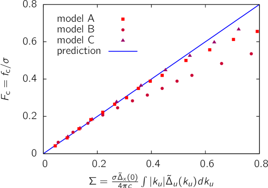
Figure 2: (Colour online) Critical force as a function of the dimensionless disorder amplitude $\Sigma$, defined in (40): comparison between numerical simulations and analytical prediction (8) for random field (models A and B) and random bond (model C) disorders (the disorders are defined precisely in section 5.1). Points are results of the simulations and the line is the analytical prediction, valid in the small $\Sigma$ limit.

4 Analytical computation

In this section, we start by computing the average force required to drive the line at an average speed $v$ with a spring of stiffness $\kappa$. This provides us a force-velocity characteristic curve that depends on the spring stiffness. From these characteristic curves, we deduce that sending the velocity and stiffness to zero in the appropriate order allows to extract the critical force.

4.1 Drag force

The line evolution equation (1) is highly non linear due to the presence of the random potential; it is thus very difficult to handle. To evaluate the average drag, we resort to a perturbative analysis in the disorder amplitude $\sigma$.

We expand the line position in powers of $\sigma$ as

$$u(t)=\sum_{n}\sigma^{n}u_{n}(t).$$ (9)

At order $0$, the solution of (1) is independent of disorder

$$u_{0}(x,t)=vt-\frac{v}{\kappa},$$ (10)

leading from (7) to the average drag

$$f_{\mathrm{dr}}^{(0)}(\kappa,v)=v.$$ (11)

The computation at higher orders is done in Fourier space, with the convention $\tilde{g}(k_{x})=\int g(x)\mathrm{e}^{-ik_{x}x}\mathrm{d}x$ (and similarly along direction $u$). We start by Fourier transforming the elastic force,

$$f_{\mathrm{el}}[u(\cdot,t)](x)=-c\int|k_{x}|\tilde{u}(k_{x},t)\mathrm{e}^{ik_{x}x}\frac{\mathrm{d}k_{x}}{2\pi},$$ (12)

and the disorder correlator,

$$\overline{\tilde{V}(k_{x},k_{u})\tilde{V}(k_{x}^{\prime},k_{u}^{\prime})}=\\ (2\pi)^{2}\delta(k_{x}+k_{x}^{\prime})\delta(k_{u}+k_{u}^{\prime})\tilde{R}_{x}(k_{x})\tilde{R}_{u}(k_{u}).$$ (13)

We also define, corresponding to (4-5)

$$\tilde{\Delta}_{x}(k_{x}) =\tilde{R}_{x}(k_{x}),$$ (14)

$$\tilde{\Delta}_{u}(k_{u}) =k_{u}^{2}\tilde{R}_{u}(k_{u}).$$ (15)

The first order contribution to the line position satisfies

$$\partial_{t}u_{1}(x,t)+\kappa u_{1}(x,t)-f_{\mathrm{el}}[u_{1}(\cdot,t)](x)=-\partial_{u}V(x,u_{0}(t)).$$ (16)

Fourier transforming this equation in directions $x$ and $u$ gives the solution in Fourier space

$$\tilde{u}_{1}(k_{x},t)=-\int\frac{ik_{u}}{ik_{u}v+\omega(k_{x})}\mathrm{e}^{ik_{u}u_{0}(t)}\tilde{V}(k_{x},k_{u})\frac{\mathrm{d}k_{u}}{2\pi},$$ (17)

where we have introduced the damping rate

$$\omega(k_{x})=\kappa+c|k_{x}|,$$ (18)

which fully encompasses the effect of the elasticity. Since the first order correction is linear in the potential $V$, its average over disorder is 0 and it does not contribute to the drag: $f_{\mathrm{dr}}^{(1)}=0$.

At second order, the evolution equation reads

$$\partial_{t}u_{2}(x,t)+ \kappa u_{2}(x,t)-f_{\mathrm{el}}[u_{2}(\cdot,t)](x)=$$ (19)

$$-\sigma^{-1}[\partial_{u}V(x,u_{0}(t)+\sigma u_{1}(x,t))-\partial_{u}V(x,u_{0}(t))].$$

Following an idea introduced by Larkin [27], we expand the potential around $u_{0}(t)$, getting

$$\partial_{t}u_{2}(x,t)+\kappa u_{2}(x,t)-f_{\mathrm{el}}[u_{2}(\cdot,t)](x)=-\partial_{u}^{2}V(x,u_{0}(t))u_{1}(x,t).$$ (20)

It reads in Fourier space

$$\partial_{t}\tilde{u}_{2}(k_{x},t)+ \omega(k_{x})\tilde{u}_{2}(k_{x},t)=$$ (21)

$$\int k_{u}^{2}\mathrm{e}^{ik_{u}u_{0}(t)}\tilde{V}(k_{x}^{\prime},k_{u})\tilde{u}_{1}(k_{x}-k_{x}^{\prime},t)\frac{\mathrm{d}k_{x}^{\prime}\mathrm{d}k_{u}}{(2\pi)^{2}}.$$

Inserting the first order result (17) and solving gives

$$\tilde{u}_{2}(k_{x},t)= \int\frac{ik_{u}^{\prime 2}(k_{u}^{\prime}-k_{u})\mathrm{e}^{ik_{u}u_{0}(t)}}{[ik_{u}v+\omega(k_{x})][i(k_{u}-k_{u}^{\prime})v+\omega(k_{x}-k_{x}^{\prime})]}$$ (22)

$$\ \qquad\times\tilde{V}(k_{x}-k_{x}^{\prime},k_{u}-k_{u}^{\prime})\tilde{V}(k_{x}^{\prime},k_{u}^{\prime})\frac{\mathrm{d}k_{x}^{\prime}\mathrm{d}k_{u}\mathrm{d}k_{u}^{\prime}}{(2\pi)^{3}}.$$

Averaging over disorder with (13) leads to

$$\overline{\tilde{u}_{2}(k_{x})}=2\pi\delta(k_{x})\int\frac{ik_{u}\tilde{\Delta}_{x}(k_{x}^{\prime})\tilde{\Delta}_{u}(k_{u})}{\kappa[-ik_{u}v+\omega(k_{x}^{\prime})]}\frac{\mathrm{d}k_{x}^{\prime}\mathrm{d}k_{u}}{(2\pi)^{2}}.$$ (23)

The proportionality to $\delta(k_{x})$ signifies that, in direct space, the average second order correction does not depend on the internal coordinate $x$. It reads

$$\overline{u_{2}}=-\int\frac{vk_{u}^{2}\tilde{\Delta}_{x}(k_{x})\tilde{\Delta}_{u}(k_{u})}{\kappa[k_{u}^{2}v^{2}+\omega(k_{x})^{2}]}\frac{\mathrm{d}k_{x}\mathrm{d}k_{u}}{(2\pi)^{2}}.$$ (24)

The second order drag is thus:

$$f_{\mathrm{dr}}^{(2)}(v,\kappa)=\sigma^{2}\int\frac{vk_{u}^{2}\tilde{\Delta}_{x}(k_{x})\tilde{\Delta}_{u}(k_{u})}{k_{u}^{2}v^{2}+(\kappa+c|k_{x}|)^{2}}\frac{\mathrm{d}k_{x}\mathrm{d}k_{u}}{(2\pi)^{2}}.$$ (25)

Adding this result to the zeroth order drag (11) provides the drag up to the order $\sigma^{2}$,

$$f_{\mathrm{dr,2}}(v,\kappa) =f_{\mathrm{dr}}^{(0)}(v,\kappa)+f_{\mathrm{dr}}^{(1)}(v,\kappa)+f_{\mathrm{dr}}^{(2)}(v,\kappa)$$ (26)

$$=v+\sigma^{2}\int\frac{vk_{u}^{2}\tilde{\Delta}_{x}(k_{x})\tilde{\Delta}_{u}(k_{u})}{k_{u}^{2}v^{2}+(\kappa+c|k_{x}|)^{2}}\frac{\mathrm{d}k_{x}\mathrm{d}k_{u}}{(2\pi)^{2}}.$$ (27)

This drag gives us access, at the perturbative level, to the crucial force-velocity characteristic. It is plotted on Fig. 3 for a random field disorder with Gaussian two-point functions, at different values of the spring stiffness. When the spring stiffness $\kappa$ goes to zero, the depinning transition appears clearly and becomes sharp when $\kappa=0$. The picture is qualitatively similar for a random bond disorder. Any positive stiffness rounds the transition, analogously to the temperature [4, 28, 14].

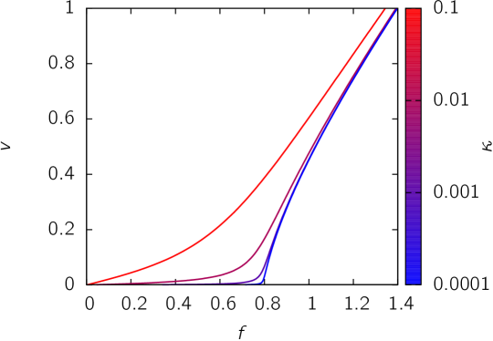
Figure 3: (Colour online) Force-velocity curve using the drag (27) computed to the second order in $\sigma$, for different values of the parabola curvature $\kappa$, indicated by the colour scale. The two-point functions $\Delta_{x}$ and $\Delta_{u}$ of the disorder are centered Gaussian functions of unit variance, encoding a random field disorder.

4.2 Critical force

As noted above, the usual force-velocity characteristic at zero temperature is recovered in the limit $\kappa\rightarrow 0$; its equation is given by

$$f_{\kappa=0,2}(v)=v+\frac{\sigma^{2}}{c}\int\frac{k_{u}^{2}\tilde{\Delta}_{x}(vq/c)\tilde{\Delta}_{u}(k_{u})}{k_{u}^{2}+q^{2}}\frac{\mathrm{d}q\mathrm{d}k_{u}}{(2\pi)^{2}}.$$ (28)

We have performed the variable substitution $ck_{x}=vq$ in order to eliminate the velocity in the denominator. Taking the small velocity limit in this expression gives the critical force (8)

$$f_{\mathrm{c,2}}=\frac{\sigma^{2}\tilde{\Delta}_{x}(0)}{4\pi c}\int|k_{u}|\tilde{\Delta}_{u}(k_{u})\mathrm{d}k_{u}.$$ (29)

This expression is our main result, announced in Eq. (8). The index $2$ indicates that this critical force comes from a second order perturbative computation in the disorder amplitude $\sigma$. The two limits do not commute: since any non-zero stiffness rounds the transition, taking the limit of zero velocity first would give a zero critical force (see Fig. 3). To get the depinning exponent $\beta$ defined by $v\sim_{f\rightarrow f_{\mathrm{c}}^{+}}(f-f_{\mathrm{c}})^{\beta}$, we have to go one step further in the Taylor expansion of (28) around $v=0$. This can be done analytically for simple correlators $\tilde{\Delta}_{x}(k_{x})$ and $\tilde{\Delta}_{u}(k_{u})$, or numerically in the general case (see Fig. 3 for an example). We get

$$v\sim f-f_{\mathrm{c}},$$ (30)

which corresponds to the mean field behaviour ${\beta=\beta_{\mathrm{MF}}=1}$ [29] valid above the upper critical dimension $d_{\mathrm{uc}}$ (for the long-range elasticity $d_{\mathrm{uc}}=2$). Below $d_{\mathrm{uc}}$, the mean field value $\beta_{\mathrm{MF}}=1$ is an upper bound of the exact value of $\beta$ which can be estimated by a functional renormalization group $\epsilon-$expansion [30, 31, 32] or evaluated numerically to $\beta=0.625\pm 0.0005$ for the long-range elastic line [33].

5 Numerical simulations

We now turn to the comparison of our analytical prediction to numerical simulations of the line. Since our computation remains valid for both random bond and random field disorder, we perform numerical simulations on both cases.

5.1 Numerical model

In our model a line of length $L$ is discretized with a step $a$ and its elasticity is given by

$$f_{\mathrm{el}}[u(\cdot,t)]_{n}=\frac{c}{\pi a}\sum_{n^{\prime}\neq 0}\frac{u_{n^{\prime}}(t)-u_{n}(t)}{(n-n^{\prime})^{2}}.$$ (31)

Each point of the line moves on a rail with a disordered potential which is uncorrelated with the others rails, so that $\Delta_{x}(x-x^{\prime})=\delta_{x,x^{\prime}}$. Three different models of disorder are considered:

• model A: random field disorder obtained by the linear interpolation of the random force drawn at the extremities of segments of length $1$;

• model B: random field disorder obtained in the same way as model A, but the segments have length $0.1$ with probability $1/2$ and $1.9$ with probability $1/2$;

• model C: random bond disorder obtained by the spline interpolation of the random energies drawn at the extremities of segments of length $1$.

5.2 Analytical prediction

The prediction of the critical force for the three models can be obtained observing that for a discrete line the damping rate (18) changes to

$$\omega(k_{x})=\kappa+c\left(|k_{x}|-\frac{ak_{x}^{2}}{2\pi}\right).$$ (32)

where the wave-vector $k_{x}$ is restricted to $\left[-\pi/a,\pi/a\right]$. The limits $\kappa\rightarrow 0$ and $v\rightarrow 0$ give exactly the same result as (8):

$$f_{\mathrm{c,2}}=\lim_{v\rightarrow 0}\lim_{\kappa\rightarrow 0}f_{\mathrm{tot,2}}(v,\kappa)=\frac{\sigma^{2}\tilde{\Delta}_{x}(0)}{4\pi c}\int|k_{u}|\tilde{\Delta}_{u}(k_{u})\mathrm{d}k_{u}.$$ (33)

It is remarkable that discretizing the line does not change the critical force. In all models we set $a=1$ so that $\tilde{\Delta}_{x}(0)=1$ and the functional of $\Delta_{u}(u)$ appearing in our expression (8) for the critical force is computed in A for the three models. The final prediction for model A is:

$$f_{\mathrm{c,2}}=\frac{2\log(2)}{\pi}\frac{\sigma^{2}}{c}\simeq 0.44\frac{\sigma^{2}}{c}.$$ (34)

while for model B a numerical computation gives

$$f_{\mathrm{c,2}}\simeq 0.55\frac{\sigma^{2}}{c},$$ (35)

and for model C we have

$$f_{\mathrm{c,2}}\simeq 2.83\frac{\sigma^{2}}{c}.$$ (36)

5.3 Measurement of the critical force

We start our numerical procedure with a flat configuration $u(x)=0$ and $w=0$. Then the interface moves to a state, $u_{w=0}(x)$ which is stable with respect to small deformations. Increasing $w$, the interface position increases and a sequence of stable states can be recorded. For each $w$, the stable state $u_{w}(x)$ can be found using the algorithm proposed in [34] and we measure the pinning force

$$f_{w}(\kappa)=\kappa[w-\langle u_{w}(x)\rangle].$$ (37)

This pinning force depends on the realization of the disordered potential (its fluctuations have been studied in [35]). An example of the evolution of the pinning force with $w$ is shown on Fig. 4. The pinning force is in general dependent on the initial condition, however, due to the Middleton no-passing rule [36], we can prove that there exists a $w^{*}>0$ such that the sequence of stable states $u_{w>w^{*}}(x)$ becomes independent of the initial condition. A stationary state is thus reached, where the pinning force oscillates around its average value $\overline{f(\kappa)}$ and displays correlation in $w$. Thus in order to estimate correctly $\overline{f(\kappa)}$ we sample $f_{w}(\kappa)$ far enough from the origin $w=0$ and for values of $w$ far enough from each other.

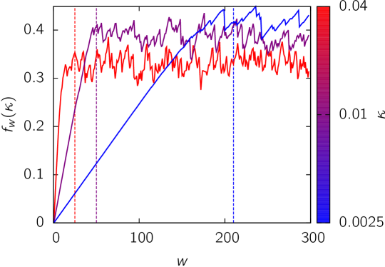
Figure 4: (Colour online) Pinning force (37) as a function of the position $w$ of the parabola, for different values of the spring stiffness $\kappa$. The dashed vertical lines represent approximate values $w^{*}$ after which the pinning force becomes independent of the initial condition. Model A disorder with $\sigma=1$ is used here.

An exact relation (the statistical tilt symmetry [37]) assures that the quadratic part of the Hamiltonian (and thus the constant $\kappa$) is not renormalized. This means that the length associated by a simple dimensional analysis to the bare constant $\kappa$, namely $L_{\kappa}=c/\kappa$, corresponds to the correlation length of the system: above $L_{\kappa}$ the interface is flat and feels the harmonic parabola only, while below $L_{\kappa}$ the interface is rough with the characteristic roughness exponent at depinning $\zeta\simeq 0.39$ [34].

The separation from the critical depinning point (located exactly at the critical driving force $f_{\mathrm{c}}$) is described by the power law scaling [38] $f-f_{\mathrm{c}}\sim\xi^{-1/\nu}$ where $\xi$ is the correlation length, given in our case by $L_{\kappa}$. When $\kappa\to 0$ (while keeping $L\gg L_{\kappa}$) the pinning force tends to the thermodynamical critical force $f_{\mathrm{c}}$. Gathering the previous scalings, we thus have that the finite size effects on the force take the form:

$$\overline{f(\kappa)}=f_{\mathrm{c}}+c_{1}\kappa^{1/\nu}+\cdots.$$ (38)

The fluctuations around this value, $\overline{\delta f(\kappa)^{2}}$, depend on $L$ and $\kappa$. In the limit $L\gg L_{\kappa}=1/\kappa$, the interface can be modeled as a collection of independent interfaces of size $L_{\kappa}$ and the central limit theorem assures that the variance $\overline{\delta f(\kappa)^{2}}$ should scale as $\sim\kappa^{2/\nu}$, but with an extra factor $L_{\kappa}/L$. This allows us to write an extrapolation formula for $f_{\mathrm{c}}$ which is independent of the critical exponent $\nu$:

$$\overline{f(\kappa)}=f_{\mathrm{c}}+c_{1}\sqrt{\kappa L\overline{\delta f(\kappa)^{2}}}+\cdots$$ (39)

Our determination of $f_{\mathrm{c}}$ is performed using this relation, by extrapolating the numerical measurements of $\overline{f(\kappa)}$ for different values of $\kappa$ to the limit $\kappa\to 0$, as shown on Fig. 5. It is worth noticing that most of the details of the finite size system such as the boundary conditions or the presence of the parabolic well does not affect the thermodynamic value of $f_{\mathrm{c}}$ which depends only on the elastic constant $c$ and on the disorder statistics [39, 40]. Our extrapolation of $f_{\mathrm{c}}$, shown on Fig. 5, has been performed on samples of size $L=1000,4000$ (depending on the value of sigma) and for parabola curvatures down to $\kappa=10^{-4}$.

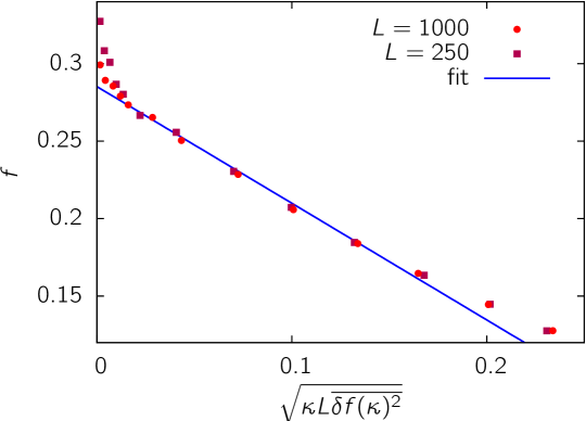
Figure 5: (Colour online) Pinning force averaged over the parabola position $w$, versus a function of the spring stiffness. A fit of the linear part gives the critical force, see Eq. (39). This plot is for model A disorder with $\sigma=0.8$ and we found $f_{\mathrm{c}}=0.285$.

5.4 Results

The dimensionless critical force $F_{\mathrm{c}}=f_{\mathrm{c}}/\sigma$ is plotted versus the dimensionless disorder parameter

$$\Sigma=\frac{\sigma\tilde{\Delta}_{x}(0)}{4\pi c}\int|k_{u}|\tilde{\Delta}_{u}(k_{u})\mathrm{d}k_{u}$$ (40)

on Fig. 2. In all three cases, the results are very close to the theoretical prediction $F_{\mathrm{c}}=\Sigma$ (equivalent to (8)) when the disorder parameter is small.

6 Conclusion

We have shown that the critical force for a long-range elastic line in a random landscape can be computed perturbatively in the collective pinning regime, yielding the expression (8). Our result for the critical force gives, together with its scaling with respect to the microscopic parameters, its dependence on the disorder geometry. Indeed, we have shown that two disorders that can be attributed the same correlation lengths (as in model A and B) may present a different critical force that is precisely predicted by our theory.

Some previous studies have studied the scaling of the critical force with respect to microscopic parameters such as the disorder amplitude $\sigma$, the elastic constant $c$ and disorder correlation lengths $\xi_{x}$ and $\xi_{u}$ in the directions $x$ and $u$ [5, 21, 24]. In particular for the long-range elastic line, the following scaling has been found for the critical force in the collective pinning regime [24]:

$$f_{\mathrm{c}}\sim\frac{\sigma^{2}\xi_{x}}{c\xi_{u}}.$$ (41)

The lengths $\xi_{x}$ and $\xi_{u}$ characterize the typical scale of the disorder correlation along $x$ and $u$, but these scales cannot be uniquely defined. Different definitions lead to correlation lengths that differ only by a numerical factor, so the scaling law (41) holds independently of the chosen definitions. However, this prevents the use this scaling law to make a quantitative prediction. Our formula allows to overcome this problem. In particular, starting from Eq. (8) and writing

$$\Delta_{x}(x)=\Delta_{x1}(x/\xi_{x})$$ (42)

where $\Delta_{x1}$ is a function of the dimensionless variable $x/\xi_{x}$ and a similar relation defines $\Delta_{u1}$, one gets

$$f_{\mathrm{c}}=\left(\frac{\tilde{\Delta}_{x1}(0)}{4\pi}\int|q_{u}|\tilde{\Delta}_{u1}(q_{u})\mathrm{d}q_{u}\right)\times\frac{\sigma^{2}\xi_{x}}{c\xi_{u}}.$$ (43)

This shows that our analytical prediction (8) allows to recover the scaling law (41) and gives additionally the prefactor as a function of the correlation functions, i.e. it yields the explicit dependence of the critical force on the disorder geometry.

The present work is not the first attempt to compute the critical force perturbatively: expansions have been performed at weak disorder [41, 18], small temperature [28] or large velocity [42, 43]. Weak disorder expansions are valid up to the Larkin length [5], $L_{c}$ defined as the distance at which the line wanders enough to see the finite disorder correlation length $\xi_{u}$, (namely $|u(L_{c})-u(0)|\simeq\xi_{u}$). Above the Larkin length, they however predict an incorrect roughness exponent [44]. Last, large velocity expansions give an estimation of the critical force that is obtained by continuing a large-velocity asymptotic result, which lies very far from the depinning regime, to zero velocity. Our computation does not need such continuation, and is compatible with the fact that perturbative expansions in the disorder amplitude are incorrect above the Larkin length, since the critical force can be evaluated from the line behaviour at the scale of the Larkin length [5].

Our analysis is a first step towards a more general understanding of the critical force dependence, and it can be extended in several directions. First, the opposite individual pinning regime occurring at a high disorder amplitude is worth investigating. The perturbative analysis used here is not suited for its study, but a few comments can be made on the grounds of former numerical studies [24, 25]. First, its scaling with respect to the disorder amplitude and correlation length has been elucidated for a long-range elastic line, giving [24]

$$f_{\mathrm{c}}\sim\sigma;$$ (44)

thus the critical force is now proportional to the disorder amplitude and does not depend on the disorder correlation lengths. Moreover, we have shown in a previous study [24] that the critical force is given by the strongest pinning sites if the pinning force is bounded. In this case, it is likely that the dependence on the disorder geometry is very weak. The case of unbounded pinning force requires further investigation.

Another issue arising from our study is the question of the landscape smoothness. Our analysis requires an expansion of the potential to the second order around the position of the unperturbed line (see Eq. (20)): the force generated by the potential must be continuous. When one tries to apply the analytical prediction (8) to a discontinuous force landscape, it diverges because of a cusp present in the correlation function $\Delta_{u}(u)$. On the other hand, our previous numerical study [24] used a discontinuous force landscape and did not reveal any divergence, while the dependence on the disorder amplitude, $f_{\mathrm{c}}\sim\sigma^{2}$, was the same as the one observed here. This suggests that the divergence obtained when we try to apply our result to a discontinuous force landscape is regularized by a mechanism that is out of reach of the present perturbative computation. Understanding the behaviour of the elastic line and the critical force in a rougher force landscape would be an important advance on a theoretical point of view, but also for experiments where discontinuous force landscapes are ubiquitous [8, 11].

Last, the case of a short-range instead of long-range elasticity remains to be understood within our approach; interesting comparison could be established with the characteristic force of the creep-regime, whose dependency in the details of the disorder correlator (for RB disorder) has been examined recently [45, 46, 47].

Appendix A Disorder generation and correlation

We detail here the procedures used to generate the different models of disorder, and how to compute the disorder correlation function, that is needed to evaluate the critical force (8).

A.1 Random field disorder: models A and B

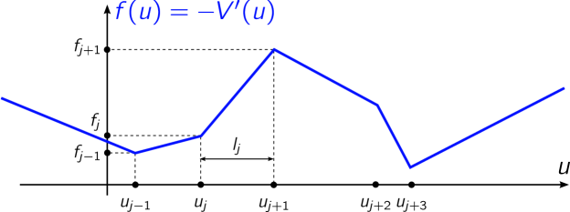
Figure 6: (Colour online) Random force disorder on a rail: the force is continuous and piecewise linear.

For a random force disorder, the disorder is generated on each rail using the following procedure (see Fig. 6):

• The rail is divided into segments of random length $l$ drawn in the distribution $P(l)$.

• At the point linking the segment $j-1$ and the segment $j$, a random force $f_{j}$ is drawn from a Gaussian distribution with zero mean and unit variance.

• Inside the segment $j$, at a generic point $u$, the force $f(u)$, is obtained by the linear interpolation such that $f(u_{j})=f_{j}$ and $f(u_{j+1})=f_{j+1}$.

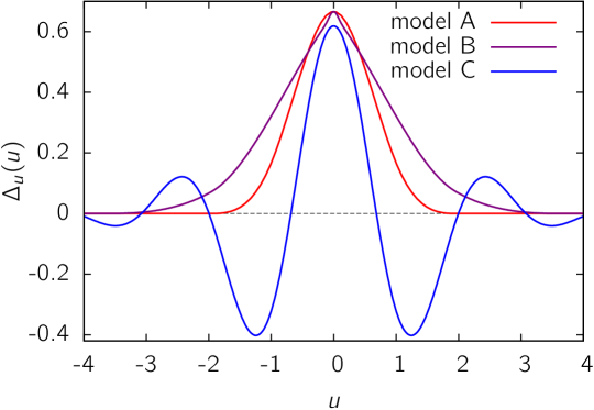
Figure 7: (Colour online) Two-point correlation function of the force $\Delta_{u}(u)=\overline{\partial_{u}V(0)\partial_{u}V(u)}$ for the disorder models A, B and C. The model C correlation function has been rescaled by a factor $0.25$.

We want to know the correlation of the forces at two points separated by a distance $u\geq 0$, say $f(0)$ and $f(u)$. This correlation is non-zero if the two points lie on the same segment or on neighbour segments. We introduce the length $l$ of the segment where the point $0$ lies, the length $l^{\prime}$ of its right neighbour, and the left end $u_{0}$ of the first segment. The probability distribution for $l$ is $Q(l)=lP(l)/\bar{l}$, where $\bar{l}=\int_{0}^{\infty}P(l)dl$; the probability distribution for $l^{\prime}$ is simply $P(l^{\prime})$ and the one of $u_{0}$ is $l^{-1}\chi_{[-l,0]}(u_{0})$ (meaning that the point $0$ is uniformly distributed in its segment). Putting these probabilities together, we get the probability distribution for $(l,l^{\prime},u_{0})$:

$$\mathbb{P}(l,l^{\prime},u_{0})=\bar{l}^{-1}P(l)P(l^{\prime})\chi_{[-l,0]}(u_{0}).$$ (45)

The points $0$ and $u$ are on the same segment if ${u\leq u_{0}+l}$. The force at $u_{0}$ is $f_{0}$ and the force at $u_{0}+l$ is $f_{1}$; $f_{0}$ and $f_{1}$ are uncorrelated random variables with zero mean and unit variance. The forces at $0$ and $u$ are

$$f(0) =f_{0}\frac{u_{0}+l}{l}+f_{1}\frac{-u_{0}}{l},$$ (46)

$$f(u) =f_{0}\frac{u_{0}+l-u}{l}+f_{1}\frac{u-u_{0}}{l}.$$ (47)

The correlation between these two forces is

$$\overline{f(0)f(u)}=\frac{2u_{0}^{2}+2(l-u)u_{0}+l^{2}}{l^{2}}.$$ (49)

Here, the average is restricted to the forces $f_{0}$ and $f_{1}$, the other variables $l$, $l^{\prime}$ and $u_{0}$ are fixed. On the other hand, when $u_{0}+l\leq u\leq u_{0}+l+l^{\prime}$, the two points lie on neighbour segments. The same argument gives for the force correlation

$$\overline{f(0)f(u)}=\frac{-u_{0}^{2}-(l+l^{\prime}-u)u_{0}}{ll^{\prime}}.$$ (50)

Gathering the results (45,49,50) and integrating over $u_{0}$ gives for the correlation function:

$$\Delta_{u}(u)=\frac{1}{\bar{l}}\int_{0}^{\infty}\mathrm{d}lP(l)\left(\chi_{[0,l]}(u)\frac{u^{3}-3l^{2}u+2l^{3}}{3l^{2}}+\vphantom{\left[\frac{-2u_{0}^{3}-3(l+l^{\prime}-u)u_{0}^{2}}{6ll^{\prime}}\right]^{\min(u-l,0)}_{\max(u-l-l^{\prime},-l)}}\right.$$

$$\left.\int_{0}^{\infty}\mathrm{d}l^{\prime}P(l^{\prime})\chi_{[0,l+l^{\prime}]}(u)\left[\frac{-2u_{0}^{3}-3(l+l^{\prime}-u)u_{0}^{2}}{6ll^{\prime}}\right]^{\min(u-l,0)}_{\max(u-l-l^{\prime},-l)}\right),$$ (51)

where we have used the notation $[g(u_{0})]_{a}^{b}=g(b)-g(a)$.

For the model A, all the segments have the same length $l=1$, corresponding to the probability density

$$P(l)=\delta(l-1),$$ (52)

For the model B, the segment lengths can take two values, $0.1$ and $1.9$, with probability $1/2$ each:

$$P(l)=\frac{1}{2}\delta(l-0.1)+\frac{1}{2}\delta(l-1.9).$$ (53)

For the model A, inserting the probability density (52) in the general formula (A.1) gives the correlation function for $u\geq 0$,

$$\Delta_{u}(u)=\chi_{[0,1]}(u)\frac{3u^{3}-6u^{2}+4}{6}+\chi_{(1,2]}(u)\frac{(2-u)^{3}}{6},$$ (54)

it is plotted on Fig. 7. To compute the critical force (8), we need the following quantity,

$$\int|k_{u}|\tilde{\Delta}_{u}(k_{u})\mathrm{d}k_{u} =4\int_{0}^{\infty}\frac{\Delta_{u}(0)-\Delta_{u}(u)}{u^{2}}\mathrm{d}u$$ (55)

$$=8\log(2).$$

For the model B, the correlation function is more complex and is plotted on Fig. 7. The integral entering the expression (8) of the critical force has to be computed numerically; we get

$$\int|k_{u}|\tilde{\Delta}_{u}(k_{u})\mathrm{d}k_{u}\simeq 6.91.$$ (56)

A.2 Random bond disorder: model C

A random bond disorder can be generated on a rail by drawing random energies for points on a grid of step $l$. A spline interpolation of these energies then allows to get a smooth landscape of potential. We determine here the two-point correlation function of such a disorder (see [47] for a similar study for a two-dimensional spline). Specifically, let us consider a grid of spacing $l$ with $2n+1$ points indexed from $-n$ to $n$. A random value $V_{i}$ is attached to each site $u_{i}=il$ of the grid. The function $V(u)$ is a cubic spline of the $(V_{i})_{-n\leq i\leq n}$, that is:

• $V(u)$ is a cubic polynomial on each lattice segment $[u_{i},u_{i+1}]$ for $-n\leq i<n$,

• $V(u)$ is continuous on each lattice site $u_{i}$, and equal to $V_{i}$: $V(u_{i}^{+})=V(u_{i}^{-})=V_{i}$ ,

• the first and second derivatives of $V(u)$ are continuous: $V^{\prime}(u_{i}^{+})=V^{\prime}(u_{i}^{-})$ and $V^{\prime\prime}(u_{i}^{+})=V^{\prime\prime}(u_{i}^{-})$.

One defines the coefficients $A_{i}^{0},\ldots,A_{i}^{3}$ ($-n\leq i<n$) of the polynomials as

$$V(u)=A_{i}^{0}+A_{i}^{1}(u-u_{i})+\frac{A_{i}^{2}}{2}(u-u_{i})^{2}+\frac{A_{i}^{3}}{3!}(u-u_{i})^{3}$$ (57)

for $u_{i}\leq u<u_{i+1}$. One has $A_{i}^{0}=V_{i}$.

Denoting $l_{i}=u_{i+1}-u_{i}$ (not needed to be constant, we will keep it generic for a while), the continuity conditions write:

$$A_{i+1}^{0} =A_{i}^{0}+l_{i}A_{i}^{1}+\frac{1}{2}l_{i}^{2}A_{i}^{2}+\frac{1}{3!}l_{i}^{3}A_{i}^{3}\>,$$ (58)

$$A_{i+1}^{1} =A_{i}^{1}+l_{i}A_{i}^{2}+\frac{1}{2}l_{i}^{2}A_{i}^{3}\>,$$ (59)

$$A_{i+1}^{2} =A_{i}^{2}+l_{i}A_{i}^{3}\>.$$ (60)

There are $6n$ unknown variables and $6n-2$ of those bulk equations. They have to be complemented by boundary conditions (e.g. fixing the values of the derivatives at extremities, or imposing periodic boundary conditions). The simplest way to solve the set of equations is to eliminate the $A_{i}^{1}$’s and the $A_{i}^{3}$’s to obtain equations on the $A_{i}^{2}$’s only, as a function of the parameters $l_{i}$ and $A_{i}^{0}=V_{i}$. From (60) one has $A_{i}^{3}=({A_{i+1}^{2}-A_{i}^{2}})/{l_{i}}$ and substituting into (58) one obtains $A_{i}^{1}$:

$$A_{i}^{1}=\frac{A_{i+1}^{0}-A_{i}^{0}}{l_{i}}-l_{i}\frac{2A_{i}^{2}+A_{i+1}^{2}}{6}.$$ (61)

Using these expressions in (59) one gets the equations on the $A_{i}^{2}$’s:

$$l_{i}A_{i}^{2}+2(l_{i}+l_{i+1})A_{i+1}^{2}+ l_{i+1}A_{i+2}^{2}=$$ (62)

$$6\frac{A_{i+2}^{0}-A_{i+1}^{0}}{l_{i+1}}-6\frac{A_{i+1}^{0}-A_{i}^{0}}{l_{i}}.$$

Those are quite complex to solve in general but simplifications occur for an uniform spacing $l_{i}=l$ and in the infinite grid size limit $n\to\infty$.

Solution for constant $l_{i}=l$: The equations write

$$A_{i}^{2}+4A_{i+1}^{2}+A_{i+2}^{2}=\frac{6}{h^{2}}\big{(}A_{i}^{0}-2A_{i+1}^{0}+A_{i+2}^{0}\big{)}.$$ (63)

They take the form $M\vec{A^{2}}=\frac{6}{h^{2}}\Delta\vec{A^{0}}$ where $\Delta$ is the discrete Laplacian and $M$ is a tridiagonal $(2n+1)\times(2n+1)$ matrix. It is best represented as $M=6(\mathbf{1}+\frac{1}{6}\Delta)$ with

$$\Delta=\left(\begin{array}[]{ccccc}-2&1&0&0&\ldots\\ 1&-2&1&0&\ldots\\ 0&1&-2&1&\\ \vdots&&\ddots&\ddots&\ddots\end{array}\right)$$ (64)

which allows to invert $M$ by writing:

$$M^{-1}=\frac{1}{6}\sum_{p\geq 0}\frac{(-1)^{p}}{6^{p}}\Delta^{p}.$$ (65)

Hence, the vector $\vec{A^{2}}$ of the $A_{i}^{2}$’s is obtained as

$$\vec{A^{2}}=\frac{1}{l^{2}}\sum_{p\geq 0}\frac{(-1)^{p}}{6^{p}}\Delta^{p+1}\vec{A^{0}}.$$ (66)

Each of the $A_{i}^{2}$’s is a linear combination of all the fixed potentials $A_{i}^{0}=V_{i}$’s. It is known that the coefficients of $\Delta^{p}$ are given in the infinite size limit $n\to\infty$ by the binomial coefficients, up to a sign. For instance the diagonal and subdiagonal elements are

$$\big{(}\Delta^{p})_{ii}=(-1)^{p}\left({\begin{array}[]{c}\!\!\!{2p}\!\!\!\\ \!\!\!{p}\!\!\!\end{array}}\right)\qquad\big{(}\Delta^{p})_{i,i+1}=(-1)^{p+1}\left({\begin{array}[]{c}\!\!\!{2p}\!\!\!\\ \!\!\!{p-1}\!\!\!\end{array}}\right).$$

One is now ready to determine the correlator of the potential. On a generic interval $il\leq y\leq(i+1)l$ $(i>0)$ one has

$$V(u+\eta)= \Big{(}i+1-\frac{u}{l}\Big{)}A_{i}^{0}-\Big{(}i-\frac{u}{l}\Big{)}A_{i+1}^{0}+$$ (67)

$$\frac{(u-il)(u-(i+1)l)}{6l}\times$$

$$\big{[}((2+i)l-u)A_{i}^{2}+(u-(i-1)l)A_{i+1}^{2}\big{]}\,$$

where $\eta$ is uniformly distributed on $[0,l]$ and allows to implement the statistical invariance by translation of the disorder (and generalizes the result of [47]). To determine the correlation function $\overline{V(u)V(u^{\prime})}$, one thus has to identify the segments to which $u$ and $u^{\prime}$ belong, and expanding (67), to determine averages of the form $\overline{A_{i}^{0}A_{j}^{2}}$. Those are obtained from the large-$n$ limit explicit form of (66), which reads

$$A^{2}_{j} =\ldots+(-1)^{i}\frac{1}{l^{2}}\sum_{p\geq 0}\frac{1}{6^{p}}\left({\begin{array}[]{c}\!\!\!{2p+2}\!\!\!\\ \!\!\!{p-i+1}\!\!\!\end{array}}\right)A^{0}_{j+i}+\ldots$$ (70)

$$=\ldots+(-1)^{i+1}\frac{6\sqrt{3}}{l^{2}}\left(2-\sqrt{3}\right)^{i}A^{0}_{j+i}+\ldots$$ (71)

which yields for instance $\overline{A_{0}^{0}A_{i}^{2}}=(-1)^{i+1}\frac{6\sqrt{3}}{l^{2}}\left(2-\sqrt{3}\right)^{i}$. One obtains a cumbersome expression in real space, defined piecewise, that we do not reproduce here for clarity. After Fourier transformation, the correlator $\tilde{R}_{u}$ is found to take a simple form

$$\tilde{R}_{u}(k_{u})=\frac{9{\rm\,sinc\!}\left(\frac{k_{u}}{2}\right)^{8}}{(2+\cos(k_{u}))^{2}}\>,$$ (72)

which we have checked numerically. The force correlation function is shown on Fig. 7; unlike the random field correlation functions, it presents negative parts indicating anticorrelations of the disorder (due to the spline continuity constraints).

References

References

- [1] T. Halpin-Healy and Y.-C. Zhang. Kinetic roughening phenomena, stochastic growth, directed polymers and all that. Physics Reports 254, 215 (1995).
- [2] M. Kardar. Nonequilibrium dynamics of interfaces and lines. Physics Reports 301, 85 (1998).
- [3] S. Brazovskii and T. Nattermann. Pinning and sliding of driven elastic systems: from domain walls to charge density waves. Advances in Physics 53, 177 (2004).
- [4] E. Agoritsas, V. Lecomte, and T. Giamarchi. Disordered elastic systems and one-dimensional interfaces. Physica B: Condensed Matter 407, 1725 (2012).
- [5] A. I. Larkin and Y. N. Ovchinnikov. Pinning in type II superconductors. Journal of Low Temperature Physics 34, 409 (1979).
- [6] S. Lemerle, J. Ferré, C. Chappert, V. Mathet, T. Giamarchi, and P. Le Doussal. Domain Wall Creep in an Ising Ultrathin Magnetic Film. Phys. Rev. Lett. 80, 849 (1998).
- [7] J. F. Joanny and P. G. d. Gennes. A model for contact angle hysteresis. The Journal of Chemical Physics 81, 552 (1984).
- [8] J. Soriano, J. Ortín, and A. Hernández-Machado. Experiments of interfacial roughening in Hele-Shaw flows with weak quenched disorder. Phys. Rev. E 66, 031603 (2002).
- [9] S. Santucci, R. Planet, K. J. Måløy, and J. Ortín. Avalanches of imbibition fronts: Towards critical pinning. EPL (Europhysics Letters) 94, 46005 (2011).
- [10] E. Bouchaud, J. P. Bouchaud, D. S. Fisher, S. Ramanathan, and J. R. Rice. Can crack front waves explain the roughness of cracks? Journal of the Mechanics and Physics of Solids 50, 1703 (2002).
- [11] D. Bonamy, S. Santucci, and L. Ponson. Crackling Dynamics in Material Failure as the Signature of a Self-Organized Dynamic Phase Transition. Phys. Rev. Lett. 101, 045501 (2008).
- [12] A.-L. Barabási and H. E. Stanley. Fractal Concepts in Surface Growth. Cambridge University Press 1995.
- [13] J. Krug. Origins of scale invariance in growth processes. Advances in Physics 46, 139 (1997).
- [14] S. Bustingorry, A. B. Kolton, and T. Giamarchi. Thermal rounding of the depinning transition. EPL (Europhysics Letters) 81, 26005 (2008).
- [15] L. B. Ioffe and V. M. Vinokur. Dynamics of interfaces and dislocations in disordered media. Journal of Physics C: Solid State Physics 20, 6149 (1987).
- [16] T. Nattermann. Scaling approach to pinning: Charge density waves and giant flux creep in superconductors. Physical Review Letters 64, 2454 (1990).
- [17] L. Balents and D. S. Fisher. Large-n expansion of ()-dimensional oriented manifolds in random media. Phys. Rev. B 48, 5949–5963 (1993).
- [18] P. Chauve, T. Giamarchi, and P. Le Doussal. Creep and depinning in disordered media. Phys. Rev. B 62, 6241 (2000).
- [19] A. B. Kolton, A. Rosso, T. Giamarchi, and W. Krauth. Creep dynamics of elastic manifolds via exact transition pathways. Phys. Rev. B 79, 184207 (2009).
- [20] P. W. Anderson and Y. B. Kim. Hard Superconductivity: Theory of the Motion of Abrikosov Flux Lines. Rev. Mod. Phys. 36, 39 (1964).
- [21] T. Nattermann, Y. Shapir, and I. Vilfan. Interface pinning and dynamics in random systems. Phys. Rev. B 42, 8577 (1990).
- [22] S. Roux, D. Vandembroucq, and F. Hild. Effective toughness of heterogeneous brittle materials. European Journal of Mechanics - A/Solids 22, 743 (2003).
- [23] S. Roux and F. Hild. Self-consistent scheme for toughness homogenization. International Journal of Fracture 154, 159 (2008).
- [24] V. Démery, L. Ponson, and A. Rosso. From microstructural features to effective toughness in disordered brittle solids. ArXiv 1212.1551 (2012).
- [25] S. Patinet, D. Vandembroucq, and S. Roux. Quantitative Prediction of Effective Toughness at Random Heterogeneous Interfaces. Phys. Rev. Lett. 110, 165507 (2013).
- [26] E. E. Ferrero, S. Bustingorry, A. B. Kolton, and A. Rosso. Numerical approaches on driven elastic interfaces in random media. Comptes Rendus Physique 14, 641 (2013).
- [27] A. I. Larkin. Effect of inhomogeneities on the structure of the mixed state of superconductors. Soviet Physics JETP 31, 784 (1970).
- [28] L.-W. Chen and M. C. Marchetti. Interface motion in random media at finite temperature. Phys. Rev. B 51, 6296 (1995).
- [29] D. S. Fisher. Collective transport in random media: from superconductors to earthquakes. Physics Reports 301, 113 (1998).
- [30] P. Chauve, P. Le Doussal, and K. Jörg Wiese. Renormalization of Pinned Elastic Systems: How Does It Work Beyond One Loop? Phys. Rev. Lett. 86, 1785 (2001).
- [31] P. Le Doussal, K. J. Wiese, and P. Chauve. Functional renormalization group and the field theory of disordered elastic systems. Phys. Rev. E 69, 026112 (2004).
- [32] K. J. Wiese and P. L. Doussal. Functional renormalization for disordered systems, basic recipes and gourmet dishes. ArXiv cond-mat/0611346 2006. Markov Processes Relat. Fields 13, 777 (2007).
- [33] O. Duemmer and W. Krauth. Depinning exponents of the driven long-range elastic string. Journal of Statistical Mechanics: Theory and Experiment 2007, P01019 (2007).
- [34] A. Rosso and W. Krauth. Roughness at the depinning threshold for a long-range elastic string. Phys. Rev. E 65, 025101 (2002).
- [35] C. J. Bolech and A. Rosso. Universal statistics of the critical depinning force of elastic systems in random media. Phys. Rev. Lett. 93, 125701 (2004).
- [36] A. A. Middleton. Asymptotic uniqueness of the sliding state for charge-density waves. Phys. Rev. Lett. 68, 670 (1992).
- [37] U. Schulz, J. Villain, E. Brézin, and H. Orland. Thermal fluctuations in some random field models. Journal of Statistical Physics 51, 1 (1988).
- [38] T. Nattermann, S. Stepanow, L.-H. Tang, and H. Leschhorn. Dynamics of interface depinning in a disordered medium. J. Phys. II France 2, 1483 (1992).
- [39] A. B. Kolton, S. Bustingorry, E. E. Ferrero, and A. Rosso. Uniqueness of the thermodynamic limit for driven disordered elastic interfaces. ArXiv 1308.4329 (2013).
- [40] Z. Budrikis and S. Zapperi. Size effects in dislocation depinning models for plastic yield. Journal of Statistical Mechanics: Theory and Experiment 2013, P04029 (2013).
- [41] K. B. Efetov and A. I. Larkin. Charge-density wave in a random potential. Sov. Phys. JETP 45, 1236 (1977).
- [42] A. Schmid and W. Hauger. On the theory of vortex motion in an inhomogeneous superconducting film. Journal of Low Temperature Physics 11, 667 (1973).
- [43] A. Larkin and Y. N. Ovchinnikov. Electrodynamics of inhomogeneous type-II superconductor. JETP 38, 854 (1974).
- [44] M. Kardar. Replica Bethe ansatz studies of two-dimensional interfaces with quenched random impurities. Nuclear Physics B 290, 582 (1987).
- [45] E. Agoritsas, V. Lecomte, and T. Giamarchi. Temperature-induced crossovers in the static roughness of a one-dimensional interface. Physical Review B 82, 184207 (2010).
- [46] E. Agoritsas, V. Lecomte, and T. Giamarchi. Static fluctuations of a thick one-dimensional interface in the 1+1 directed polymer formulation. Physical Review E 87, 042406 (2013).
- [47] E. Agoritsas, V. Lecomte, and T. Giamarchi. Static fluctuations of a thick one-dimensional interface in the 1+1 directed polymer formulation: Numerical study. Phys. Rev. E 87, 062405 (2013).