Consistency of weighted majority votes

Abstract

We revisit the classical decision-theoretic problem of weighted expert voting from a statistical learning perspective. In particular, we examine the consistency (both asymptotic and finitary) of the optimal Nitzan-Paroush weighted majority and related rules. In the case of known expert competence levels, we give sharp error estimates for the optimal rule. When the competence levels are unknown, they must be empirically estimated. We provide frequentist and Bayesian analyses for this situation. Some of our proof techniques are non-standard and may be of independent interest. The bounds we derive are nearly optimal, and several challenging open problems are posed. Experimental results are provided to illustrate the theory.

1 Introduction

The problem of weighting the input of several experts arises in many situations and is of considerable theoretical and practical importance. The rigorous study of majority vote has its roots in the work of Condorcet (1785). By the 70s, the field of decision theory was actively exploring various voting rules (see Nitzan & Paroush (1982) and the references therein). A typical setting is as follows. An agent is tasked with predicting some random variable $Y\in\left\{\pm 1\right\}$ based on input $X_{i}\in\left\{\pm 1\right\}$ from each of $n$ experts. Each expert $X_{i}$ has a competence level $p_{i}\in(0,1)$, which is the probability of making a correct prediction: $\mathbb{P}(X_{i}=Y)=p_{i}$. Two simplifying assumptions are commonly made:

• Independence: The random variables $\left\{X_{i}:i\in[n]\right\}$ are mutually independent.

• Unbiased truth: $\mathbb{P}(Y=+1)=\mathbb{P}(Y=-1)=1/2$.

We will discuss these assumptions below in greater detail; for now, let us just take them as given. (Since the bias of $Y$ can be easily estimated from data, only the independence assumption is truly restrictive.) A decision rule is a mapping $f:\left\{\pm 1\right\}^{n}\to\left\{\pm 1\right\}$ from the $n$ expert inputs to the agent’s final decision. Our quantity of interest throughout the paper will be the agent’s probability of error,

$$\mathbb{P}(f(\boldsymbol{\mathrm{X}})\neq Y).$$ (1)

A decision rule $f$ is optimal if it minimizes the quantity in (1) over all possible decision rules. Nitzan & Paroush (1982) showed that, when Assumptions (i)–(ii) hold and the true competences $p_{i}$ are known, the optimal decision rule is obtained by an appropriately weighted majority vote:

$$f^{\textrm{{\tiny{OPT}}}}(\boldsymbol{\mathrm{x}})=\operatorname{sign}\left(\sum_{i=1}^{n}w_{i}x_{i}\right),$$ (2)

where the weights $w_{i}$ are given by

$$w_{i}=\log\frac{p_{i}}{1-p_{i}},\qquad i\in[n].$$ (3)

Thus, $w_{i}$ is the log-odds of expert $i$ being correct — and the voting rule in (2), also known as naive Bayes (Hastie et al., 2009), may be seen as a simple consequence of the Neyman-Pearson lemma (Neyman & Pearson, 1933).

Main results.

The formula in (2) raises immediate questions, which apparently have not previously been addressed. The first one has to do with the consistency of the Nitzan-Paroush optimal rule: under what conditions does the probability of error decay to zero and at what rate? In Section 3, we show that the probability of error is controlled by the committee potential $\Phi$, defined by

$$\Phi=\sum_{i=1}^{n}(p_{i}-{\textstyle\frac{1}{2}})w_{i}=\sum_{i=1}^{n}(p_{i}-{\textstyle\frac{1}{2}})\log\frac{p_{i}}{1-p_{i}}.$$ (4)

More precisely, we prove in Theorem 1 that

$$-\log\mathbb{P}(f^{\textrm{{\tiny{OPT}}}}(\boldsymbol{\mathrm{X}})\neq Y) \asymp \Phi,$$

where $\asymp$ denotes equivalence up to universal multiplicative constants. Another issue not addressed by the Nitzan-Paroush result is how to handle the case where the competences $p_{i}$ are not known exactly but rather estimated empirically by $\hat{p}_{i}$. We present two solutions to this problem: a frequentist and a Bayesian one. As we show in Section 4, the frequentist approach does not admit an optimal empirical decision rule. Instead, we analyze empirical decision rules in various settings: high-confidence (i.e., $|\hat{p}_{i}-p_{i}|\ll 1$) vs. low-confidence, adaptive vs. nonadaptive. The low-confidence regime requires no additional assumptions, but provides weaker guarantees (Theorem 5). In the high-confidence regime, the adaptive approach provides error estimates in terms of the empirical $\hat{p}_{i}$s (Theorem 10), while the nonadaptive approach gives a bound in terms of the unknown $p_{i}$s, but still gives useful asymptotics (Theorem 9). The Bayesian solution sidesteps the various cases above, as it admits a simple, provably optimal empirical decision rule (Section 5). Unfortunately, we are unable to compute (or even nontrivially estimate) the probability of error induced by this rule; this is posed as a challenging open problem.

2 Background and related work

Machine learning theory typically clusters weighted majority (Littlestone & Warmuth, 1989, 1994) within the framework of online algorithms; see Cesa-Bianchi & Lugosi (2006) for a modern treatment. Since the online setting is considerably more adversarial than ours, we obtain very different weighted majority rules and consistency guarantees. The weights $w_{i}$ in (2) bear a striking similarity to the Adaboost update rule (Freund & Schapire, 1997; Schapire & Freund, 2012). However, the latter assumes weak learners with access to labeled examples, while in our setting the experts are “static”. Still, we do not rule out a possible deeper connection between the Nitzan-Paroush decision rule and boosting. In a recent line of work Lacasse et al. (2006); Laviolette & Marchand (2007); Roy et al. (2011) have developed a PAC-Bayesian theory for the majority vote of simple classifiers. This approach facilitates data-dependent bounds and is even flexible enough to capture some simple dependencies among the classifiers — though, again, the latter are learners as opposed to our experts. Even more recently, experts with adversarial noise have been considered (Mansour et al., 2013). More directly related to the present work are the papers of Berend & Paroush (1998), which characterizes the consistency of the simple majority rule, and Boland et al. (1989); Berend & Sapir (2007) which analyze various models of dependence among the experts.

3 Known competences

In this section we assume that the expert competences $p_{i}$ are known and analyze the consistency of the Nitzan-Paroush optimal decision rule (2). Our main result here is that the probability of error $\mathbb{P}(f^{\textrm{{\tiny{OPT}}}}(\boldsymbol{\mathrm{X}})\neq Y)$ is small if and only if the committee potential $\Phi$ is large.

Theorem 1.

Suppose that the experts $\boldsymbol{\mathrm{X}}=(X_{1},\ldots,X_{n})$ satisfy Assumptions (i)-(ii) and $f:\left\{\pm 1\right\}^{n}\to\left\{\pm 1\right\}$ is the Nitzan-Paroush optimal decision rule. Then

• ${\displaystyle\mathbb{P}(f^{\textrm{{\tiny{OPT}}}}(\boldsymbol{\mathrm{X}})\neq Y)\leq\exp\left(-{\textstyle\frac{1}{2}}\Phi\right)}.$

• ${\displaystyle\mathbb{P}(f^{\textrm{{\tiny{OPT}}}}(\boldsymbol{\mathrm{X}})\neq Y)\geq\frac{3}{4[1+\exp(2\Phi+4\sqrt{\Phi})]}}.$

Open problem.

Exhibit (if possible) a function $g:\mathbb{R}\to\mathbb{R}$ such that

$$\mathbb{P}(f^{\textrm{{\tiny{OPT}}}}(\boldsymbol{\mathrm{X}})\neq Y) \asymp g(\Phi).$$

The remainder of this section is devoted to proving Theorem 1.

3.1 Proof of Theorem 1(i)

Define the $\left\{0,1\right\}$-indicator variables

$$\xi_{i}=\mathds{1}_{\left\{X_{i}=Y\right\}},$$ (5)

corresponding to the event that the $i$^th expert is correct. A mistake $f^{\textrm{{\tiny{OPT}}}}(\boldsymbol{\mathrm{X}})\neq Y$ occurs precisely when the sum of the correct experts’ weights fails to exceed half the total mass:

$$\mathbb{P}(f^{\textrm{{\tiny{OPT}}}}(\boldsymbol{\mathrm{X}})\neq Y)=\mathbb{P}\left(\sum_{i=1}^{n}w_{i}\xi_{i}\leq\frac{1}{2}\sum_{i=1}^{n}w_{i}\right).$$ (6)

Since $\mathbb{E}\xi_{i}=p_{i}$, we may rewrite the probability in (6) as

$$\mathbb{P}\left(\sum_{i}w_{i}\xi_{i}\leq\mathbb{E}\left[\sum_{i}w_{i}\xi_{i}\right]-\sum_{i}(p_{i}-{\textstyle\frac{1}{2}})w_{i}\right).$$ (7)

A standard tool for estimating such sum deviation probabilities is Hoeffding’s inequality. Applied to (7), it yields the bound

$$\mathbb{P}(f^{\textrm{{\tiny{OPT}}}}(\boldsymbol{\mathrm{X}})\neq Y)\leq\exp\left(-\frac{2\left[\sum_{i}(p_{i}-{\textstyle\frac{1}{2}})w_{i}\right]^{2}}{\sum_{i}w_{i}^{2}}\right),$$ (8)

which is far too crude for our purposes. Indeed, consider a finite committee of highly competent experts with $p_{i}$’s arbitrarily close to $1$ and $X_{1}$ the most competent of all. Raising $X_{1}$’s competence sufficiently far above his peers will cause both the numerator and the denominator in the exponent to be dominated by $w_{1}^{2}$, making the right-hand-side of (8) bounded away from zero. The inability of Hoeffding’s inequality to guarantee consistency even in such a felicitous setting is an instance of its generally poor applicability to highly heterogeneous sums, a phenomenon explored in some depth in McAllester & Ortiz (2003). Bernstein’s and Bennett’s inequalities suffer from a similar weakness (see ibid.). Fortunately, an inequality of Kearns & Saul (1998) is sufficiently sharp to yield the desired estimate: For all $p\in[0,1]$ and all $t\in\mathbb{R}$,

$$(1-p)e^{-tp}+pe^{t(1-p)}\leq\exp\left(\frac{1-2p}{4\log((1-p)/p)}t^{2}\right).$$ (9)

Remark 1.

The Kearns-Saul inequality (9) may be seen as a distribution-dependent refinement of Hoeffding’s (which bounds the left-hand-side of (9) by $e^{t^{2}/8}$), and is not nearly as straightforward to prove. An elementary rigorous proof is given in Berend & Kontorovich (2013b). Following up, Raginsky & Sason (2013) gave a “soft” proof based on transportation and information-theoretic techniques.

Put $\theta_{i}=\xi_{i}-p_{i}$, substitute into (6), and apply Markov’s inequality:

$$\mathbb{P}(f^{\textrm{{\tiny{OPT}}}}(\boldsymbol{\mathrm{X}})\neq Y) = \mathbb{P}\left(-\sum_{i}w_{i}\theta_{i}\geq\Phi\right)$$

$$\leq e^{-t\Phi}\mathbb{E}{\exp\left(-t\sum_{i}w_{i}\theta_{i}\right)}.$$

Now

$$\mathbb{E}e^{-tw_{i}\theta_{i}} = p_{i}e^{-(1-p_{i})w_{i}t}+(1-p_{i})e^{p_{i}w_{i}t}$$

$$\leq \exp\left(\frac{-1+2p_{i}}{4\log(p_{i}/(1-p_{i}))}w_{i}^{2}t^{2}\right)$$

$$= \exp\left[{\textstyle\frac{1}{2}}(p_{i}-{\textstyle\frac{1}{2}})w_{i}t^{2}\right],$$

where the inequality follows from (9). By independence,

$$\mathbb{E}\exp\left(-t\sum_{i}w_{i}\theta_{i}\right) = \prod_{i}\mathbb{E}e^{-tw_{i}\theta_{i}}$$

$$\leq \exp\left({\textstyle\frac{1}{2}}\sum_{i}(p_{i}-{\textstyle\frac{1}{2}})w_{i}t^{2}\right)$$

$$= \exp\left({\textstyle\frac{1}{2}}\Phi t^{2}\right)$$

and hence

$$\mathbb{P}(f^{\textrm{{\tiny{OPT}}}}(\boldsymbol{\mathrm{X}})\neq Y) \leq \exp\left({\textstyle\frac{1}{2}}\Phi t^{2}-\Phi t\right).$$

Choosing $t=1$ yields the bound in Theorem 1(i).

3.2 Proof of Theorem 1(ii)

Define the $\left\{\pm 1\right\}$-indicator variables

$$\eta_{i}=2\mathds{1}_{\left\{X_{i}=Y\right\}}-1,$$ (12)

corresponding to the event that the $i$^th expert is correct and put $q_{i}=1-p_{i}$. The shorthand $\boldsymbol{\mathrm{w}}\cdot\boldsymbol{\mathrm{\eta}}=\sum_{i=1}^{n}w_{i}\eta_{i}$ will be convenient. We will need some simple lemmata:

Lemma 2.

$$\mathbb{P}(f^{\textrm{{\tiny{OPT}}}}(\boldsymbol{\mathrm{X}})=Y)=\sum_{\boldsymbol{\mathrm{\eta}}\in\left\{\pm 1\right\}^{n}}\max\left\{P(\boldsymbol{\mathrm{\eta}}),P(-\boldsymbol{\mathrm{\eta}})\right\}$$

and

$$\mathbb{P}(f^{\textrm{{\tiny{OPT}}}}(\boldsymbol{\mathrm{X}})\neq Y)=\sum_{\boldsymbol{\mathrm{\eta}}\in\left\{\pm 1\right\}^{n}}\min\left\{P(\boldsymbol{\mathrm{\eta}}),P(-\boldsymbol{\mathrm{\eta}})\right\},$$

where

$$P(\boldsymbol{\mathrm{\eta}})=\prod_{i:\eta_{i}=1}{p_{i}}\prod_{i:\eta_{i}=-1}{q_{i}}.$$

Proof.

The identities (5), (6) and (12) imply that a mistake occurs precisely when

$$\sum_{i=1}^{n}w_{i}\frac{\eta_{i}+1}{2}\leq\frac{1}{2}\sum_{i=1}^{n}w_{i},$$

which is equivalent to

$$\boldsymbol{\mathrm{w}}\cdot\boldsymbol{\mathrm{\eta}}\leq 0.$$ (13)

Exponentiating both sides,

$$\exp\left(\boldsymbol{\mathrm{w}}\cdot\boldsymbol{\mathrm{\eta}}\right) = \prod_{i=1}^{n}e^{w_{i}\eta_{i}}$$ (14)

$$= \prod_{i:\eta_{i}=1}\frac{p_{i}}{q_{i}}\cdot\prod_{i:\eta_{i}=-1}\frac{q_{i}}{p_{i}}$$

$$= \frac{P(\boldsymbol{\mathrm{\eta}})}{P(-\boldsymbol{\mathrm{\eta}})}\leq 1.$$

We conclude from (14) that among two “antipodal” atoms $\pm\boldsymbol{\mathrm{\eta}}\in\left\{\pm 1\right\}^{n}$, the one with the greater mass contributes to the probability being correct and the one with the smaller mass contributes to the probability of error, which proves the claim. ∎

Remark 2.

The proof of Lemma 2 also establishes the optimality of the Nitzan-Paroush decision rule.

Lemma 3.

Suppose that $\boldsymbol{\mathrm{s}},\boldsymbol{\mathrm{s}}^{\prime}\in(0,\infty)^{m}$ satisfy

$$\sum_{i=1}^{m}(s_{i}+s_{i}^{\prime})\geq a$$

and

$$\frac{1}{R}\leq\frac{s_{i}}{s_{i}^{\prime}}\leq R,\qquad i\in[m]$$

for some $R<\infty$. Then

$$\sum_{i=1}^{m}\min\left\{s_{i},s_{i}^{\prime}\right\}\geq\frac{a}{1+R}.$$

Proof.

Immediate from

$$s_{i}+s_{i}^{\prime}\leq\min\left\{s_{i},s_{i}^{\prime}\right\}(1+R).$$

∎

Lemma 4.

Define the function $F:(0,1)\to\mathbb{R}$ by

$$F(x)=\frac{x(1-x)\log(x/(1-x))}{2x-1}.$$

Then $\sup_{0<x<1}F(x)={\textstyle\frac{1}{2}}$.

Proof.

Deferred to the Appendix. ∎

Continuing with the main proof, observe that

$$\mathbb{E}\left[\boldsymbol{\mathrm{w}}\cdot\boldsymbol{\mathrm{\eta}}\right]=\sum_{i=1}^{n}(p_{i}-q_{i})w_{i}=2\Phi$$ (15)

and

$$\operatorname{Var}\left[\boldsymbol{\mathrm{w}}\cdot\boldsymbol{\mathrm{\eta}}\right]=4\sum_{i=1}^{n}p_{i}q_{i}w_{i}^{2}.$$

By Lemma 4,

$$p_{i}q_{i}w_{i}^{2}\leq{\textstyle\frac{1}{2}}(p_{i}-q_{i})w_{i},$$

and hence

$$\operatorname{Var}\left[\boldsymbol{\mathrm{w}}\cdot\boldsymbol{\mathrm{\eta}}\right] \leq 4\Phi.$$ (16)

Define the segment $I\subset\mathbb{R}$ by

$$I=\left[2\Phi-4\sqrt{\Phi},2\Phi+4\sqrt{\Phi}\right].$$ (17)

Chebyshev’s inequality together with (15) and (16) implies that

$$\mathbb{P}\left(\boldsymbol{\mathrm{w}}\cdot\boldsymbol{\mathrm{\eta}}\in I\right) \geq \frac{3}{4}.$$ (18)

Consider an atom $\boldsymbol{\mathrm{\eta}}\in\left\{\pm 1\right\}^{n}$ for which $\boldsymbol{\mathrm{w}}\cdot\boldsymbol{\mathrm{\eta}}\in I$. The proof of Lemma 2 shows that

$$\frac{P(\boldsymbol{\mathrm{\eta}})}{P(-\boldsymbol{\mathrm{\eta}})}=\exp\left(\boldsymbol{\mathrm{w}}\cdot\boldsymbol{\mathrm{\eta}}\right)\leq\exp(2\Phi+4\sqrt{\Phi}),$$ (19)

where the inequality follows from (17). Lemma 2 further implies that

$$\mathbb{P}(f^{\textrm{{\tiny{OPT}}}}(\boldsymbol{\mathrm{X}})\neq Y) \geq \sum_{{\boldsymbol{\mathrm{\eta}}\in\left\{\pm 1\right\}^{n}:\boldsymbol{\mathrm{w}}\cdot\boldsymbol{\mathrm{\eta}}\in I}}\min\left\{P(\boldsymbol{\mathrm{\eta}}),P(-\boldsymbol{\mathrm{\eta}})\right\}$$

$$\geq \frac{3/4}{1+\exp(2\Phi+4\sqrt{\Phi})},$$

where the second inequality follows from Lemma 3, (18) and (19). This completes the proof.

4 Unknown competences: frequentist approach

Our goal in this section is to obtain, insofar as possible, analogues of Theorem 1 for unknown expert competences. When the ${p_{i}}$s are unknown, they must be estimated empirically before any useful weighted majority vote can be applied. There are various ways to model partial knowledge of expert competences (Baharad et al., 2011, 2012). Perhaps the simplest scenario for estimating the $p_{i}$s is to assume that the $i$^th expert has been queried independently $m_{i}$ times, out of which he gave the correct prediction $k_{i}$ times. Taking the $\left\{m_{i}\right\}$ to be fixed, define the committee profile by $\boldsymbol{\mathrm{k}}=(k_{1},\ldots,k_{n})$; this is the aggregate of the agent’s empirical knowledge of the experts’ performance. An empirical decision rule $\hat{f}:(\boldsymbol{\mathrm{x}},\boldsymbol{\mathrm{k}})\mapsto\left\{\pm 1\right\}$ makes a final decision based on the expert inputs $\boldsymbol{\mathrm{x}}$ together with the committee profile. Analogously to (1), the probability of a mistake is

$$\mathbb{P}(\hat{f}(\boldsymbol{\mathrm{X}},\boldsymbol{\mathrm{K}})\neq Y).$$ (20)

Note that now the committee profile is an additional source of randomness. Here we run into our first difficulty: unlike the probability in (1), which is minimized by the Nitzan-Paroush rule, the agent cannot formulate an optimal decision rule $\hat{f}$ in advance without knowing the ${p_{i}}$s. This is because no decision rule is optimal uniformly over the range of possible $p_{i}$s. Our approach will be to consider weighted majority decision rules of the form

$$\hat{f}(\boldsymbol{\mathrm{x}},\boldsymbol{\mathrm{k}})=\operatorname{sign}\left(\sum_{i=1}^{n}\hat{w}(k_{i})x_{i}\right)$$ (21)

and to analyze their consistency properties under two different regimes: low-confidence and high-confidence. These refer to the confidence intervals of the frequentist estimate of $p_{i}$, given by

$$\hat{p}_{i}=\frac{k_{i}}{m_{i}}.$$ (22)

4.1 Low-confidence regime

In the low-confidence regime, the sample sizes $m_{i}$ may be as small as $1$, and we define

$$\hat{w}(k_{i})=\hat{w}_{i}^{\textrm{{\tiny{LC}}}}:=\hat{p}_{i}-{\textstyle\frac{1}{2}},\qquad i\in[n],$$ (23)

which induces the empirical decision rule $\hat{f}^{\textrm{{\tiny{LC}}}}$. It remains to analyze $\hat{f}^{\textrm{{\tiny{LC}}}}$’s probability of error. Recall the definition of $\xi_{i}$ from (5) and observe that

$$\mathbb{E}\left[\hat{w}_{i}^{\textrm{{\tiny{LC}}}}\xi_{i}\right]=\mathbb{E}[(\hat{p}_{i}-{\textstyle\frac{1}{2}})\xi_{i}]=(p_{i}-{\textstyle\frac{1}{2}})p_{i},$$ (24)

since $\hat{p}_{i}$ and $\xi_{i}$ are independent. As in (6), the probability of error (20) is

$$\mathbb{P}\left(\sum_{i=1}^{n}\hat{w}_{i}^{\textrm{{\tiny{LC}}}}\xi_{i}\leq\frac{1}{2}\sum_{i=1}^{n}\hat{w}_{i}^{\textrm{{\tiny{LC}}}}\right)=\mathbb{P}\left(\sum_{i=1}^{n}Z_{i}\leq 0\right),$$ (25)

where $Z_{i}=\hat{w}_{i}^{\textrm{{\tiny{LC}}}}(\xi_{i}-{\textstyle\frac{1}{2}})$. Now the $\left\{Z_{i}\right\}$ are independent random variables, $\mathbb{E}Z_{i}=(p_{i}-{\textstyle\frac{1}{2}})^{2}$ (by (24)), and each $Z_{i}$ takes values in an interval of length ${\textstyle\frac{1}{2}}$. Hence, the standard Hoeffding bound applies:

$$\mathbb{P}(\hat{f}^{\textrm{{\tiny{LC}}}}(\boldsymbol{\mathrm{X}},\boldsymbol{\mathrm{K}})\neq Y)\leq\exp\left[-\frac{8}{n}\left(\sum_{i=1}^{n}(p_{i}-{\textstyle\frac{1}{2}})^{2}\right)^{2}\right].$$ (26)

We summarize these calculations in

Theorem 5.

A sufficient condition for $\mathbb{P}(\hat{f}^{\textrm{{\tiny{LC}}}}(\boldsymbol{\mathrm{X}},\boldsymbol{\mathrm{K}})\neq Y)\to 0$ is

$$\frac{1}{\sqrt{n}}\sum_{i=1}^{n}(p_{i}-{\textstyle\frac{1}{2}})^{2}\to\infty.$$

Several remarks are in order. First, notice that the error bound in (26) is stated in terms of the unknown $\left\{p_{i}\right\}$, providing the agent with large-committee asymptotics but giving no finitary information; this limitation is inherent in the low-confidence regime. Secondly, the condition in Theorem 5 is considerably more restrictive than the consistency condition $\Phi\to\infty$ implicit in Theorem 1. Indeed, the empirical decision rule $\hat{f}^{\textrm{{\tiny{LC}}}}$ is incapable of exploiting a single highly competent expert in the way that $f^{\textrm{{\tiny{OPT}}}}$ from (2) does. Our analysis could be sharpened somewhat for moderate sample sizes $\left\{m_{i}\right\}$ by using Bernstein’s inequality to take advantage of the low variance of the $\hat{p}_{i}$s. For sufficiently large sample sizes, however, the high-confidence regime (discussed below) begins to take over. Finally, there is one sense in which this case is “easier” to analyze than that of known $\left\{p_{i}\right\}$: since the summands in (25) are bounded, Hoeffding’s inequality gives nontrivial results and there is no need for more advanced tools such as the Kearns-Saul inequality (9) (which is actually inapplicable in this case).

4.2 High-confidence regime

In the high-confidence regime, each estimated competence $\hat{p}_{i}$ is close to the true value $p_{i}$ with high probability. To formalize this, fix some $0<\delta<1$, $0<\varepsilon\leq 5$, and put

$$q_{i}=1-p_{i},~{}\hat{q}_{i}=1-\hat{p}_{i}.$$

We will set the empirical weights according to the “plug-in” Nitzan-Paroush rule

$$\hat{w}_{i}^{\textrm{{\tiny{HC}}}}:=\log\frac{\hat{p}_{i}}{\hat{q}_{i}},\qquad i\in[n],$$ (27)

which induces the empirical decision rule $\hat{f}^{\textrm{{\tiny{HC}}}}$ and raises immediate concerns about $\hat{w}_{i}^{\textrm{{\tiny{HC}}}}=\pm\infty$. We give two kinds of bounds on $\mathbb{P}(\hat{f}^{\textrm{{\tiny{HC}}}}\neq Y)$: nonadaptive and adaptive. In the nonadaptive analysis, we show that for $m_{i}\min\left\{p_{i},q_{i}\right\}_{i}\gg 1$, with high probability $\left|w_{i}-\hat{w}_{i}^{\textrm{{\tiny{HC}}}}\right|\ll 1$, and thus a “perturbed” version of Theorem 1(i) holds (and in particular, $w_{i}^{\textrm{{\tiny{HC}}}}$ will be finite with high probability). In the adaptive analysis, we allow $\hat{w}_{i}^{\textrm{{\tiny{HC}}}}$ to take on infinite values and show (perhaps surprisingly) that this decision rule also asymptotically achieves the rate of Theorem 1(i).

Nonadaptive analysis.

Define $\tilde{\varepsilon}\in(0,1)$ by $\varepsilon=2\tilde{\varepsilon}+4\tilde{\varepsilon}^{2}$ or, explicitly,

$$\tilde{\varepsilon}=\frac{\sqrt{4\varepsilon+1}-1}{4}.$$ (28)

Lemma 6.

If

$$\tilde{\varepsilon}^{2}m_{i}p_{i} \geq 3\log({2n}/{\delta}),\qquad i\in[n],$$ (29)

then

$$\mathbb{P}\left(\exists i\in[n]:\frac{\hat{p}_{i}}{p_{i}}\notin(1-\tilde{\varepsilon},1+\tilde{\varepsilon})\right)\leq\delta.$$

Proof.

The multiplicative Chernoff bound yields

$$\mathbb{P}\left(\hat{p}_{i}<(1-\tilde{\varepsilon})p_{i}\right)\leq e^{-\tilde{\varepsilon}^{2}m_{i}p_{i}/2}$$

and

$$\mathbb{P}\left(\hat{p}_{i}>(1+\tilde{\varepsilon})p_{i}\right)\leq e^{-\tilde{\varepsilon}^{2}m_{i}p_{i}/3}.$$

Hence,

$$\mathbb{P}\left(\frac{\hat{p}_{i}}{p_{i}}\notin(1-\tilde{\varepsilon},1+\tilde{\varepsilon})\right) \leq 2e^{-\tilde{\varepsilon}^{2}m_{i}p_{i}/3}.$$

The claim follows from (29) and the union bound. ∎

Lemma 7.

Let $w_{i}$ be the optimal Nitzan-Paroush weight (3). If

$$1-\tilde{\varepsilon}\leq\frac{\hat{p}_{i}}{p_{i}},\frac{\hat{q}_{i}}{q_{i}}\leq 1+\tilde{\varepsilon}$$

then

$$\left|w_{i}-\hat{w}_{i}^{\textrm{{\tiny{HC}}}}\right|\leq\varepsilon.$$

Proof.

We have

$$\left|w_{i}-\hat{w}_{i}^{\textrm{{\tiny{HC}}}}\right| = \left|\log\frac{p_{i}}{q_{i}}-\log\frac{\hat{p}_{i}}{\hat{q}_{i}}\right|$$

$$= \left|\log\frac{p_{i}}{\hat{p}_{i}}-\log\frac{\hat{q}_{i}}{q_{i}}\right|$$

$$= \left|\log\frac{p_{i}}{\hat{p}_{i}}\right|+\left|\log\frac{\hat{q}_{i}}{q_{i}}\right|.$$

Now

$$[\log(1-\tilde{\varepsilon}),\log(1+\tilde{\varepsilon})] \subseteq [-\tilde{\varepsilon}-2\tilde{\varepsilon}^{2},\tilde{\varepsilon}]$$

$$\subseteq [-{\textstyle\frac{1}{2}}\varepsilon,{\textstyle\frac{1}{2}}\varepsilon],$$

whence

$$\left|\log\frac{p_{i}}{\hat{p}_{i}}\right|+\left|\log\frac{\hat{q}_{i}}{q_{i}}\right|\leq\varepsilon.$$

∎

Corollary 8.

If

$$\tilde{\varepsilon}^{2}m_{i}\min\left\{p_{i},q_{i}\right\}_{i} \geq 3\log({4n}/{\delta}),\qquad i\in[n],$$

then

$$\mathbb{P}\left(\max_{i\in[n]}\left|w_{i}-\hat{w}_{i}^{\textrm{{\tiny{HC}}}}\right|>\varepsilon\right) \leq \delta.$$

Proof.

An immediate consequence of applying Lemma 6 to $p_{i}$ and $q_{i}$ with the union bound. ∎

To state the next result, let us arrange the plug-in weights (27) as a vector $\hat{\boldsymbol{\mathrm{w}}}^{\textrm{{\tiny{HC}}}}\in\mathbb{R}^{n}$, as was done with $\boldsymbol{\mathrm{w}}$ and $\boldsymbol{\mathrm{\eta}}$ from Section 3.1. The corresponding weighted majority rule $\hat{f}^{\textrm{{\tiny{HC}}}}$ yields an error precisely when

$$\hat{\boldsymbol{\mathrm{w}}}^{\textrm{{\tiny{HC}}}}\cdot\boldsymbol{\mathrm{\eta}}\leq 0$$

(cf. (13)). Our nonadaptive approach culminates in the following result.

Theorem 9.

Let $0<\delta<1$ and $0<\varepsilon<\min\left\{5,2\Phi/n\right\}$. If

$$m_{i}\min\left\{p_{i},q_{i}\right\}_{i}\geq 3\left(\frac{\sqrt{4\varepsilon+1}-1}{4}\right)^{-2}\log\frac{4n}{\delta},\qquad i\in[n],$$ (30)

then

$$\mathbb{P}\left(\hat{f}^{\textrm{{\tiny{HC}}}}(\boldsymbol{\mathrm{X}},\boldsymbol{\mathrm{K}})\neq Y\right)\;\leq\;\delta+\exp\left[-\frac{(2\Phi-\varepsilon n)^{2}}{8\Phi}\right].$$ (31)

Remark 3.

For fixed $\left\{p_{i}\right\}$ and $\min_{i\in[n]}m_{i}\to\infty$, we may take $\delta$ and $\varepsilon$ arbitrarily small — and in this limiting case, the bound of Theorem 1(i) is recovered.

Proof of Theorem 9.

Since

$$\left|\boldsymbol{\mathrm{w}}\cdot\boldsymbol{\mathrm{\eta}}-\hat{\boldsymbol{\mathrm{w}}}^{\textrm{{\tiny{HC}}}}\cdot\boldsymbol{\mathrm{\eta}}\right| = \left|(\boldsymbol{\mathrm{w}}-\hat{\boldsymbol{\mathrm{w}}}^{\textrm{{\tiny{HC}}}})\cdot\boldsymbol{\mathrm{\eta}}\right|$$

$$\leq \sum_{i=1}^{n}\left|w_{i}-w_{i}^{\textrm{{\tiny{HC}}}}\right|=\left\|\boldsymbol{\mathrm{w}}-\hat{\boldsymbol{\mathrm{w}}}^{\textrm{{\tiny{HC}}}}\right\|_{1},$$

we have

$$\mathbb{P}\left(\hat{\boldsymbol{\mathrm{w}}}^{\textrm{{\tiny{HC}}}}\cdot\boldsymbol{\mathrm{\eta}}\leq 0\right)\leq\mathbb{P}(\left\|\boldsymbol{\mathrm{w}}-\hat{\boldsymbol{\mathrm{w}}}^{\textrm{{\tiny{HC}}}}\right\|_{1}>\varepsilon n)+\mathbb{P}(\boldsymbol{\mathrm{w}}\cdot\boldsymbol{\mathrm{\eta}}\leq\varepsilon n).$$

Corollary 8 upper-bounds the first term on the right-hand side by $\delta$. The second term is estimated by replacing $\Phi$ by $\Phi-\varepsilon n$ in (3.1) and repeating the argument following that formula. ∎

Adaptive analysis.

Theorem 9 has the drawback of being nonadaptive, in that its assumptions (30) and conclusions (31) depend on the unknown $\left\{p_{i}\right\}$ and hence cannot be evaluated by the agent (the bound in (26) is also nonadaptive). In the adaptive approach, all results are stated in terms of empirically observed quantities:

Theorem 10.

Put

$$\delta=\sum_{i=1}^{n}\frac{1}{\sqrt{m_{i}}}$$

and let $R$ be the event

$$\exp\left(-\frac{1}{2}\sum_{i=1}^{n}(\hat{p}_{i}-{\textstyle\frac{1}{2}})\hat{w}_{i}^{\textrm{{\tiny{HC}}}}\right) \leq \frac{\delta}{2}.$$ (32)

Then

$$\mathbb{P}\left(R\cap\left\{\hat{f}^{\textrm{{\tiny{HC}}}}(\boldsymbol{\mathrm{X}},\boldsymbol{\mathrm{K}})\neq Y\right\}\right) \leq \delta.$$

Remark 4.

Our interpretation for Theorem 10 is as follows. The agent observes the committee profile $\boldsymbol{\mathrm{K}}$, which determines the $\left\{\hat{p}_{i},\hat{w}_{i}^{\textrm{{\tiny{HC}}}}\right\}$, and then checks whether the event $R$ has occurred. If not, the adaptive agent refrains from making a decision (and may choose to fall back on the low-confidence approach described previously). If $R$ does hold, however, the agent predicts $Y$ according to $\hat{f}^{\textrm{{\tiny{HC}}}}$. As explained above, there does not exist a nontrivial a priori upper bound on $\mathbb{P}(\hat{f}^{\textrm{{\tiny{HC}}}}(\boldsymbol{\mathrm{X}},\boldsymbol{\mathrm{K}})\neq Y)$ absent any knowledge of the ${p_{i}}$s. Instead, Theorem 10 bounds the probability of the agent being “fooled” by an unrepresentative committee profile. Observe that for $\min_{i\in[n]}m_{i}\gg 1$, we have $\hat{p}_{i}\approx p_{i}$ and $\hat{w}_{i}^{\textrm{{\tiny{HC}}}}\approx w_{i}$, and thus Theorem 1(i) is recovered as a limiting case. Note that we have done nothing to prevent $\hat{w}_{i}^{\textrm{{\tiny{HC}}}}=\pm\infty$, and this may indeed happen. Intuitively, there are two reasons for infinite $\hat{w}_{i}^{\textrm{{\tiny{HC}}}}$: (a) noisy $\hat{p}_{i}$ due to $m_{i}$ being too small, or (b) the $i$^th expert is actually highly (in)competent, which causes $\hat{p}_{i}\in\left\{0,1\right\}$ even for large $m_{i}$. The $1/{\sqrt{m_{i}}}$ term in the bound ensures against case (a), while in case (b), choosing infinite $\hat{w}_{i}^{\textrm{{\tiny{HC}}}}$ causes no harm (as we show in the proof).

Proof.

We will write the probability and expectation operators with subscripts (such as $\boldsymbol{\mathrm{K}}$) to indicate the random variable(s) being summed over. Thus,

$$\mathbb{P}_{\boldsymbol{\mathrm{K}},\boldsymbol{\mathrm{X}},Y}\left(R\cap\left\{\hat{f}^{\textrm{{\tiny{HC}}}}(\boldsymbol{\mathrm{X}},\boldsymbol{\mathrm{K}})\neq Y\right\}\right) = \mathbb{P}_{\boldsymbol{\mathrm{K}},\boldsymbol{\mathrm{\eta}}}\left(R\cap\left\{\hat{\boldsymbol{\mathrm{w}}}^{\textrm{{\tiny{HC}}}}\cdot\boldsymbol{\mathrm{\eta}}\leq 0\right\}\right)$$

$$= \mathbb{E}_{\boldsymbol{\mathrm{K}}}\left[\mathds{1}_{R}\cdot\mathbb{P}_{\boldsymbol{\mathrm{\eta}}}\left(\hat{\boldsymbol{\mathrm{w}}}^{\textrm{{\tiny{HC}}}}\cdot\boldsymbol{\mathrm{\eta}}\leq 0\,|\,\boldsymbol{\mathrm{K}}\right)\right].$$

Recall that the random variable $\boldsymbol{\mathrm{\eta}}\in\left\{\pm 1\right\}^{n}$, with probability mass function

$$P(\boldsymbol{\mathrm{\eta}})=\prod_{i:\eta_{i}=1}{p_{i}}\prod_{i:\eta_{i}=-1}{q_{i}},$$

is independent of $\boldsymbol{\mathrm{K}}$, and hence

$$\mathbb{P}_{\boldsymbol{\mathrm{\eta}}}\left(\hat{\boldsymbol{\mathrm{w}}}^{\textrm{{\tiny{HC}}}}\cdot\boldsymbol{\mathrm{\eta}}\leq 0\,|\,\boldsymbol{\mathrm{K}}\right)=\mathbb{P}_{\boldsymbol{\mathrm{\eta}}}\left(\hat{\boldsymbol{\mathrm{w}}}^{\textrm{{\tiny{HC}}}}\cdot\boldsymbol{\mathrm{\eta}}\leq 0\right).$$ (34)

Define the random variable $\hat{\boldsymbol{\mathrm{\eta}}}\in\left\{\pm 1\right\}^{n}$ (conditioned on $\boldsymbol{\mathrm{K}}$) by the probability mass function

$$P(\hat{\boldsymbol{\mathrm{\eta}}})=\prod_{i:\eta_{i}=1}{\hat{p}_{i}}\prod_{i:\eta_{i}=-1}{\hat{q}_{i}},$$

and the set $A\subseteq\left\{\pm 1\right\}^{n}$ by $A=\left\{\boldsymbol{\mathrm{x}}:\hat{\boldsymbol{\mathrm{w}}}^{\textrm{{\tiny{HC}}}}\cdot\boldsymbol{\mathrm{x}}\leq 0\right\}.$ Now

$$\left|\mathbb{P}_{\boldsymbol{\mathrm{\eta}}}\left(\hat{\boldsymbol{\mathrm{w}}}^{\textrm{{\tiny{HC}}}}\cdot\boldsymbol{\mathrm{\eta}}\leq 0\right)-\mathbb{P}_{\hat{\boldsymbol{\mathrm{\eta}}}}\left(\hat{\boldsymbol{\mathrm{w}}}^{\textrm{{\tiny{HC}}}}\cdot\hat{\boldsymbol{\mathrm{\eta}}}\leq 0\right)\right| = \left|\mathbb{P}_{\boldsymbol{\mathrm{\eta}}}\left(A\right)-\mathbb{P}_{\hat{\boldsymbol{\mathrm{\eta}}}}\left(A\right)\right|$$

$$\leq \max_{A\subseteq\left\{\pm 1\right\}^{n}}\left|\mathbb{P}_{\boldsymbol{\mathrm{\eta}}}\left(A\right)-\mathbb{P}_{\hat{\boldsymbol{\mathrm{\eta}}}}\left(A\right)\right|$$

$$= \left\|\mathbb{P}_{\boldsymbol{\mathrm{\eta}}}-\mathbb{P}_{\hat{\boldsymbol{\mathrm{\eta}}}}\right\|_{\textrm{{\tiny{TV}}}}$$

$$\leq \sum_{i=1}^{n}\left|p_{i}-\hat{p}_{i}\right|=:M,$$

where the inequality follows from a standard tensorization property of the total variation norm $\left\|\cdot\right\|_{\textrm{{\tiny{TV}}}}$, see e.g. (Kontorovich, 2012, Lemma 2.2). By Theorem 1(i), we have

$$\mathbb{P}_{\hat{\boldsymbol{\mathrm{\eta}}}}\left(\hat{\boldsymbol{\mathrm{w}}}^{\textrm{{\tiny{HC}}}}\cdot\hat{\boldsymbol{\mathrm{\eta}}}\leq 0\right)\leq\exp\left(-{\textstyle\frac{1}{2}}\sum_{i=1}^{n}(\hat{p}_{i}-{\textstyle\frac{1}{2}})\hat{w}_{i}^{\textrm{{\tiny{HC}}}}\right),$$

and hence

$$\mathbb{P}_{\boldsymbol{\mathrm{\eta}}}\left(\hat{\boldsymbol{\mathrm{w}}}^{\textrm{{\tiny{HC}}}}\cdot\boldsymbol{\mathrm{\eta}}\leq 0\right)\leq M+\exp\left(-{\textstyle\frac{1}{2}}\sum_{i=1}^{n}(\hat{p}_{i}-{\textstyle\frac{1}{2}})\hat{w}_{i}^{\textrm{{\tiny{HC}}}}\right).$$

Invoking (34), we substitute the right-hand side above into (LABEL:eq:EP-decomp) to obtain

$$\mathbb{P}_{\boldsymbol{\mathrm{K}},\boldsymbol{\mathrm{X}},Y}\left(R\cap\left\{\hat{f}^{\textrm{{\tiny{HC}}}}(\boldsymbol{\mathrm{X}},\boldsymbol{\mathrm{K}})\neq Y\right\}\right) \leq \mathbb{E}_{\boldsymbol{\mathrm{K}}}\left[\mathds{1}_{R}\cdot\left(M+\exp\left(-{\textstyle\frac{1}{2}}\sum_{i=1}^{n}(\hat{p}_{i}-{\textstyle\frac{1}{2}})\hat{w}_{i}^{\textrm{{\tiny{HC}}}}\right)\right)\right]$$

$$\leq \mathbb{E}_{\boldsymbol{\mathrm{K}}}[M]+\mathbb{E}_{\boldsymbol{\mathrm{K}}}\left[\mathds{1}_{R}\exp\left(-{\textstyle\frac{1}{2}}\sum_{i=1}^{n}(\hat{p}_{i}-{\textstyle\frac{1}{2}})\hat{w}_{i}^{\textrm{{\tiny{HC}}}}\right)\right].$$

By the definition of $R$, the second term on the last right-hand side is upper-bounded by $\delta/2$. To estimate $M$, we invoke a simple mean absolute deviation bound (cf. Berend & Kontorovich (2013a)):

$$\mathbb{E}_{\boldsymbol{\mathrm{K}}}\left|p_{i}-\hat{p}_{i}\right|\;\leq\;\sqrt{\frac{p_{i}(1-p_{i})}{m_{i}}}\;\leq\;\frac{1}{2\sqrt{m_{i}}},$$

which finishes the proof. ∎

Remark 5.

The improvement mentioned in Footnote 5 is achieved via a refinement of the bound $\left\|\mathbb{P}_{\boldsymbol{\mathrm{\eta}}}-\mathbb{P}_{\hat{\boldsymbol{\mathrm{\eta}}}}\right\|_{\textrm{{\tiny{TV}}}}\leq\sum_{i=1}^{n}\left|p_{i}-\hat{p}_{i}\right|$ to $\left\|\mathbb{P}_{\boldsymbol{\mathrm{\eta}}}-\mathbb{P}_{\hat{\boldsymbol{\mathrm{\eta}}}}\right\|_{\textrm{{\tiny{TV}}}}\leq\alpha\left(\left\{\left|p_{i}-\hat{p}_{i}\right|:i\in[n]\right\}\right)$, where $\alpha(\cdot)$ is the function defined in Kontorovich (2012, Lemma 4.2).

Open problem.

As argued in Remark 4, Theorem 10 achieves the optimal asymptotic rate in $\left\{p_{i}\right\}$. Can the dependence on $\left\{m_{i}\right\}$ be improved, perhaps through a better choice of $\hat{\boldsymbol{\mathrm{w}}}^{\textrm{{\tiny{HC}}}}$?

5 Unknown competences: Bayesian approach

A shortcoming of Theorem 10 is that when condition $R$ fails, the agent is left with no estimate of the error probability. An alternative (and in some sense cleaner) approach to handling unknown expert competences $p_{i}$ is to assume a known prior distribution over the competence levels $p_{i}$. The natural choice of prior for a Bernoulli parameter is the Beta distribution, namely

$$p_{i}\sim\operatorname{Beta}(\alpha_{i},\beta_{i})$$

with density

$$\frac{p_{i}^{\alpha_{i}-1}q_{i}^{\beta_{i}-1}}{B(\alpha_{i},\beta_{i})},\qquad\alpha_{i},\beta_{i}>0,$$

where $q_{i}=1-p_{i}$ and $B(x,y)=\Gamma(x)\Gamma(y)/\Gamma(x+y)$. Our full probabilistic model is as follows. Each of the $n$ expert competences $p_{i}$ is drawn independently from a Beta distribution with known parameters $\alpha_{i},\beta_{i}$. Then the $i$^th expert, $i\in[n]$, is queried independently $m_{i}$ times, with $k_{i}$ correct predictions and $m_{i}-k_{i}$ incorrect ones. As before, $\boldsymbol{\mathrm{K}}=(k_{1},\ldots,k_{n})$ is the (random) committee profile. Absent direct knowledge of the $p_{i}$s, the agent relies on an empirical decision rule $\hat{f}:(\boldsymbol{\mathrm{x}},\boldsymbol{\mathrm{k}})\mapsto\left\{\pm 1\right\}$ to produce a final decision based on the expert inputs $\boldsymbol{\mathrm{x}}$ together with the committee profile $\boldsymbol{\mathrm{k}}$. A decision rule $\hat{f}^{\textrm{{\tiny{Ba}}}}$ is Bayes-optimal if it minimizes

$$\mathbb{P}(\hat{f}(\boldsymbol{\mathrm{X}},\boldsymbol{\mathrm{K}})\neq Y),$$ (35)

which is formally identical to (20) but semantically there is a difference: the probability in (35) is over the $p_{i}$ in addition to $(\boldsymbol{\mathrm{X}},Y,\boldsymbol{\mathrm{K}})$. Unlike the frequentist approach, where no optimal empirical decision rule was possible, the Bayesian approach readily admits one. For a given $\boldsymbol{\mathrm{x}}\in\left\{\pm 1\right\}$, define $I_{+}(\boldsymbol{\mathrm{x}})$ to be the set of YES votes

$$I_{+}(\boldsymbol{\mathrm{x}})=\left\{i\in[n]:x_{i}=+1\right\}$$

and $I_{-}(\boldsymbol{\mathrm{x}})=[n]\setminus I_{+}(\boldsymbol{\mathrm{x}})$ to be the set of NO votes. Let us fix some $A\subseteq[n]$, $B=[n]\setminus A$ and compute

$$\mathbb{P}(Y=+1,I_{+}(\boldsymbol{\mathrm{X}})=A,I_{-}(\boldsymbol{\mathrm{X}})=B)$$

$$=\prod_{i=1}^{n}\int_{0}^{1}\frac{p_{i}^{\alpha_{i}-1}q_{i}^{\beta_{i}-1}}{B(\alpha_{i},\beta_{i})}\binom{m_{i}}{k_{i}}p_{i}^{k_{i}}q_{i}^{m_{i}-k_{i}}p_{i}^{\mathds{1}_{\left\{i\in A\right\}}}q_{i}^{\mathds{1}_{\left\{i\in B\right\}}}dp_{i}$$

$$=\prod_{i=1}^{n}\frac{\binom{m_{i}}{k_{i}}p_{i}^{k_{i}}q_{i}^{m_{i}-k_{i}}}{B(\alpha_{i},\beta_{i})}\int_{0}^{1}p_{i}^{\alpha_{i}+k_{i}-1+\mathds{1}_{\left\{i\in A\right\}}}q_{i}^{\beta_{i}+m_{i}-k_{i}-1+\mathds{1}_{\left\{i\in B\right\}}}dp_{i}$$

$$=\prod_{i=1}^{n}\frac{\binom{m_{i}}{k_{i}}B(\alpha_{i}+k_{i}+\mathds{1}_{\left\{i\in A\right\}},\beta_{i}+m_{i}-k_{i}+\mathds{1}_{\left\{i\in B\right\}})}{B(\alpha_{i},\beta_{i})}.$$

Analogously,

$$\mathbb{P}(Y=-1,I_{+}(\boldsymbol{\mathrm{X}})=A,I_{-}(\boldsymbol{\mathrm{X}})=B)$$

$$=\prod_{i=1}^{n}\frac{\binom{m_{i}}{k_{i}}B(\alpha_{i}+k_{i}+\mathds{1}_{\left\{i\in B\right\}},\beta_{i}+m_{i}-k_{i}+\mathds{1}_{\left\{i\in A\right\}})}{B(\alpha_{i},\beta_{i})}.$$

Let us use the shorthand $P(+1,A,B)$ and $P(-1,A,B)$ for the joint probabilities in the last two displays, along with their corresponding conditionals $P(\pm 1\,|\,A,B)$. Obviously,

$$P(1|A,B)>P(-1|A,B)\iff P(1,A,B)>P(-1,A,B),$$

which occurs precisely if

$$\prod_{i=1}^{n}B(\alpha_{i}+k_{i}+\mathds{1}_{\left\{i\in A\right\}},\beta_{i}+m_{i}-k_{i}+\mathds{1}_{\left\{i\in B\right\}})$$

$$>\prod_{i=1}^{n}B(\alpha_{i}+k_{i}+\mathds{1}_{\left\{i\in B\right\}},\beta_{i}+m_{i}-k_{i}+\mathds{1}_{\left\{i\in A\right\}}).$$

This is equivalent to

$$\prod_{i\in A}(\alpha_{i}+k_{i})\prod_{i\in B}(\beta_{i}+m_{i}-k_{i})>\prod_{i\in B}(\alpha_{i}+k_{i})\prod_{i\in A}(\beta_{i}+m_{i}-k_{i}),$$

which further simplifies to

$$\prod_{i\in A}\frac{\alpha_{i}+k_{i}}{\beta_{i}+m_{i}-k_{i}}>\prod_{i\in B}\frac{\alpha_{i}+k_{i}}{\beta_{i}+m_{i}-k_{i}}.$$

Hence, the choice

$$\hat{w}_{i}^{\textrm{{\tiny{Ba}}}}=\log\frac{\alpha_{i}+k_{i}}{\beta_{i}+m_{i}-k_{i}}$$

guarantees that the decision rule

$$\hat{f}^{\textrm{{\tiny{Ba}}}}(\boldsymbol{\mathrm{x}},\boldsymbol{\mathrm{k}})=\operatorname{sign}\left(\sum_{i=1}^{n}\hat{w}_{i}^{\textrm{{\tiny{Ba}}}}x_{i}\right)$$

maximizes the probability of being correct for each input $\boldsymbol{\mathrm{x}}\in\left\{\pm 1\right\}^{n}$. Notice that for $0<p_{i}<1$, we have

$$\hat{w}_{i}^{\textrm{{\tiny{Ba}}}}{\mathop{\longrightarrow}\limits_{m_{i}\to\infty}}w_{i},\qquad i\in[n],$$

almost surely, both in the frequentist and the Bayesian interpretations. Unfortunately, although

$$\mathbb{P}(\hat{f}^{\textrm{{\tiny{Ba}}}}(\boldsymbol{\mathrm{X}},\boldsymbol{\mathrm{K}})\neq Y)=\mathbb{P}(\hat{\boldsymbol{\mathrm{w}}}^{\textrm{{\tiny{Ba}}}}\cdot\boldsymbol{\mathrm{\eta}}\leq 0)$$

is a deterministic function of $\left\{\alpha_{i},\beta_{i},m_{i}\right\}$, we are unable to compute it at this point, or even give a non-trivial bound. One source of the problem is the coupling between $\hat{\boldsymbol{\mathrm{w}}}^{\textrm{{\tiny{Ba}}}}$ and $\boldsymbol{\mathrm{\eta}}$.

Open problem.

Give a non-trivial estimate for $\mathbb{P}(\hat{f}^{\textrm{{\tiny{Ba}}}}(\boldsymbol{\mathrm{X}},\boldsymbol{\mathrm{K}})\neq Y)$.

6 Experiments

It is most instructive to take the committee size $n$ to be small when comparing the different voting rules. Indeed, for a large committee of “marginally competent” experts with $p_{i}={\textstyle\frac{1}{2}}+\gamma$ for some $\gamma>0$, even the simple majority rule $f^{\textrm{{\tiny{MAJ}}}}(\boldsymbol{\mathrm{x}})=\operatorname{sign}(\sum_{i=1}^{n}x_{i})$ has a probability of error decaying as $\exp(-4n\gamma^{2})$, as can be easily seen from Hoeffding’s bounds. The more sophisticated voting rules discussed in this paper perform even better in this setting. Hence, small committees provide the natural test-bed for gauging a voting rule’s ability to exploit highly competent experts. In our experiments, we set $n=5$ and the sample sizes $m_{i}$ were identical for all experts. The results were averaged over $10^{5}$ trials. Two of our experiments are described below.

Low vs. high confidence.

The goal of this experiment was to contrast the extremal behavior of $\hat{f}^{\textrm{{\tiny{LC}}}}$ vs. $\hat{f}^{\textrm{{\tiny{HC}}}}$. To this end, we numerically optimized the $\boldsymbol{\mathrm{p}}\in[0,1]^{n}$ so as to maximize the absolute gap

$$\Delta_{n}(\boldsymbol{\mathrm{p}}):=\mathbb{P}(f^{\textrm{{\tiny{LC}}}}(\boldsymbol{\mathrm{X}})\neq Y)-\mathbb{P}(f^{\textrm{{\tiny{OPT}}}}(\boldsymbol{\mathrm{X}})\neq Y),$$

where $f^{\textrm{{\tiny{LC}}}}(\boldsymbol{\mathrm{x}})=\operatorname{sign}\left(\sum_{i=1}^{n}(p_{i}-{\textstyle\frac{1}{2}})x_{i}\right)$. We were surprised to discover that, though the ratio $\mathbb{P}(f^{\textrm{{\tiny{LC}}}}(\boldsymbol{\mathrm{X}})\neq Y)/\mathbb{P}(f^{\textrm{{\tiny{OPT}}}}(\boldsymbol{\mathrm{X}})\neq Y)$ can be made arbitrarily large by setting $p_{1}\approx 1$ and the remaining $p_{i}<1-\varepsilon$, the absolute gap appears to be rather small: we conjecture (with some heuristic justification) that $\sup_{n\geq 1}\sup_{\boldsymbol{\mathrm{p}}\in[0,1]^{n}}\Delta_{n}(\boldsymbol{\mathrm{p}})=1/16$. For $\hat{f}^{\textrm{{\tiny{Ba}}}}$, we used $\alpha_{i}=\beta_{i}=1$ for all $i$. The results are reported in Figure 1.

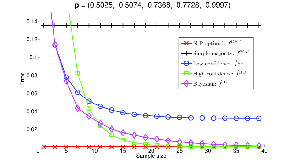
Figure 1: For very small sample sizes, $\hat{f}^{\textrm{{\tiny{LC}}}}$ outperforms $\hat{f}^{\textrm{{\tiny{HC}}}}$ but is outperformed by $\hat{f}^{\textrm{{\tiny{Ba}}}}$. Starting from sample size $\approx 13$, $\hat{f}^{\textrm{{\tiny{HC}}}}$ dominates the other empirical rules. The empirical rules are (essentially) sandwiched between $f^{\textrm{{\tiny{OPT}}}}$ and $f^{\textrm{{\tiny{MAJ}}}}$.

Bayesian setting.

In each trial, a vector of expert competences $\boldsymbol{\mathrm{p}}\in[0,1]^{n}$ was drawn independently componentwise, with $p_{i}\sim\operatorname{Beta}(1,1)$. These values (i.e., $\alpha_{i}=\beta_{i}\equiv 1$) were used for $\hat{f}^{\textrm{{\tiny{Ba}}}}$. The results are reported in Figure 2.

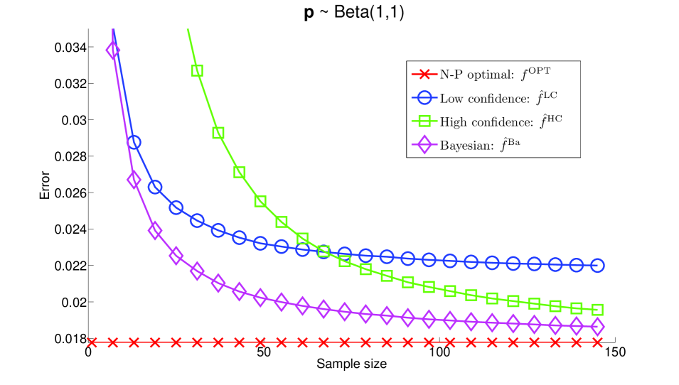
Figure 2: Unsurprisingly, $\hat{f}^{\textrm{{\tiny{Ba}}}}$ uniformly outperforms the other two empirical rules. We found it somewhat surprising that $\hat{f}^{\textrm{{\tiny{HC}}}}$ required so many samples (about $60$ on average) to overtake $\hat{f}^{\textrm{{\tiny{LC}}}}$. The simple majority rule $f^{\textrm{{\tiny{MAJ}}}}$ (off the chart) performed at an average accuracy of $50\%$, as expected.

7 Discussion

The classic and seemingly well-understood problem of the consistency of weighted majority votes continues to reveal untapped depth and suggest challenging unresolved questions. We hope that the results and open problems presented here will stimulate future research.

Appendix: Deferred proofs

Proof of Lemma 4.

Since $F$ is symmetric about $x={\textstyle\frac{1}{2}}$, it suffices to prove the claim for ${\textstyle\frac{1}{2}}\leq x<1$. We will show that $F$ is concave by examining its second derivative:

$$F^{\prime\prime}(x)=-\frac{2x-1-2x(1-x)\log(x/(1-x))}{x(1-x)(2x-1)^{3}}.$$

The denominator is obviously nonnegative on $[{\textstyle\frac{1}{2}},1]$, while the numerator has the Taylor expansion

$$\sum_{n=1}^{\infty}\frac{2^{2(n+1)}(x-{\textstyle\frac{1}{2}})^{2n+1}}{4n^{2}-1}\geq 0,\qquad{\textstyle\frac{1}{2}}\leq x<1$$

(verified through tedious but straightforward calculus). Since $F$ is concave and symmetric about ${\textstyle\frac{1}{2}}$, its maximum occurs at $F({\textstyle\frac{1}{2}})={\textstyle\frac{1}{2}}$. ∎

References

- Audibert et al. (2007) Audibert, Jean-Yves, Munos, Rémi, and Szepesvári, Csaba. Tuning bandit algorithms in stochastic environments. In ALT, pp. 150–165, 2007.
- Baharad et al. (2011) Baharad, Eyal, Goldberger, Jacob, Koppel, Moshe, and Nitzan, Shmuel. Distilling the wisdom of crowds: weighted aggregation of decisions on multiple issues. Autonomous Agents and Multi-Agent Systems, 22(1):31–42, 2011.
- Baharad et al. (2012) Baharad, Eyal, Goldberger, Jacob, Koppel, Moshe, and Nitzan, Shmuel. Beyond condorcet: optimal aggregation rules using voting records. Theory and Decision, 72(1):113–130, 2012. ISSN 0040-5833. doi: 10.1007/s11238-010-9240-5. URL http://dx.doi.org/10.1007/s11238-010-9240-5.
- Berend & Kontorovich (2013a) Berend, Daniel and Kontorovich, Aryeh. A sharp estimate of the binomial mean absolute deviation with applications. Statistics & Probability Letters, 83(4):1254–1259, 2013a.
- Berend & Kontorovich (2013b) Berend, Daniel and Kontorovich, Aryeh. On the concentration of the missing mass. Electron. Commun. Probab., 18:no. 3, 1–7, 2013b. ISSN 1083-589X. doi: 10.1214/ECP.v18-2359. URL http://ecp.ejpecp.org/article/view/2359.
- Berend & Paroush (1998) Berend, Daniel and Paroush, Jacob. When is Condorcet’s jury theorem valid? Soc. Choice Welfare, 15(4):481–488, 1998.
- Berend & Sapir (2007) Berend, Daniel and Sapir, Luba. Monotonicity in Condorcet’s jury theorem with dependent voters. Social Choice and Welfare, 28(3):507–528, 2007.
- Boland et al. (1989) Boland, Philip J., Proschan, Frank, and Tong, Y. L. Modelling dependence in simple and indirect majority systems. J. Appl. Probab., 26(1):81–88, 1989. ISSN 0021-9002.
- Cesa-Bianchi & Lugosi (2006) Cesa-Bianchi, Nicolò and Lugosi, Gábor. Prediction, learning, and games. Cambridge University Press, Cambridge, 2006.
- de Caritat marquis de Condorcet (1785) de Caritat marquis de Condorcet, J.A.N. Essai sur l’application de l’analyse à la probabilité des décisions rendues à la pluralité des voix. AMS Chelsea Publishing Series. Chelsea Publishing Company, 1785.
- Freund & Schapire (1997) Freund, Yoav and Schapire, Robert E. A decision-theoretic generalization of on-line learning and an application to boosting. J. Comput. Syst. Sci., 55(1):119–139, 1997. ISSN 0022-0000. doi: http://dx.doi.org/10.1006/jcss.1997.1504.
- Hastie et al. (2009) Hastie, Trevor, Tibshirani, Robert, and Friedman, Jerome. The Elements of Statistical Learning: Data Mining, Inference, and Prediction. Springer, New York, 2009. ISBN 0387848576.
- Kearns & Saul (1998) Kearns, Michael J. and Saul, Lawrence K. Large deviation methods for approximate probabilistic inference. In UAI, 1998.
- Kontorovich (2012) Kontorovich, Aryeh. Obtaining measure concentration from Markov contraction. Markov Processes and Related Fields, 4:613–638, 2012.
- Lacasse et al. (2006) Lacasse, Alexandre, Laviolette, François, Marchand, Mario, Germain, Pascal, and Usunier, Nicolas. PAC-Bayes bounds for the risk of the majority vote and the variance of the gibbs classifier. In NIPS, pp. 769–776, 2006.
- Laviolette & Marchand (2007) Laviolette, François and Marchand, Mario. PAC-Bayes risk bounds for stochastic averages and majority votes of sample-compressed classifiers. Journal of Machine Learning Research, 8:1461–1487, 2007.
- Littlestone & Warmuth (1989) Littlestone, Nick and Warmuth, Manfred K. The weighted majority algorithm. In FOCS, pp. 256–261, 1989.
- Littlestone & Warmuth (1994) Littlestone, Nick and Warmuth, Manfred K. The weighted majority algorithm. Inf. Comput., 108(2):212–261, 1994.
- Mansour et al. (2013) Mansour, Yishay, Rubinstein, Aviad, and Tennenholtz, Moshe. Robust aggregation of experts signals. 2013.
- Maurer & Pontil (2009) Maurer, Andreas and Pontil, Massimiliano. Empirical Bernstein bounds and sample-variance penalization. In COLT, 2009.
- McAllester & Ortiz (2003) McAllester, David A. and Ortiz, Luis E. Concentration inequalities for the missing mass and for histogram rule error. Journal of Machine Learning Research, 4:895–911, 2003.
- Mnih et al. (2008) Mnih, Volodymyr, Szepesvári, Csaba, and Audibert, Jean-Yves. Empirical Bernstein stopping. In ICML, pp. 672–679, 2008.
- Neyman & Pearson (1933) Neyman, Jerzy and Pearson, Egon S. On the problem of the most efficient tests of statistical hypotheses. Philosophical Transactions of the Royal Society A: Mathematical, Physical and Engineering Sciences, 231(694-706):289–337, 1933.
- Nitzan & Paroush (1982) Nitzan, Shmuel and Paroush, Jacob. Optimal decision rules in uncertain dichotomous choice situations. International Economic Review, 23(2):289–297, 1982.
- Raginsky & Sason (2013) Raginsky, Maxim and Sason, Igal. Concentration of measure inequalities in information theory, communications and coding. Foundations and Trends in Communications and Information Theory, 10(1-2):1–247, 2013.
- Roy et al. (2011) Roy, Jean-Francis, Laviolette, François, and Marchand, Mario. From PAC-Bayes bounds to quadratic programs for majority votes. In ICML, pp. 649–656, 2011.
- Schapire & Freund (2012) Schapire, Robert E. and Freund, Yoav. Boosting. Foundations and algorithms. Adaptive Computation and Machine Learning. Cambridge, MA: MIT Press, 2012.