Dynamical instability induced by zero mode
under symmetry breaking external perturbation

Abstract

A complex eigenvalue in the Bogoliubov-de Gennes equations for a stationary Bose-Einstein condensate in ultracold atomic system indicates the dynamical instability of the system. We also have the modes with zero eigenvalues for the condensate, called the zero modes, which originate from the spontaneous breakdown of symmetries. Although the zero modes are suppressed in many theoretical analyses, we take account of them in this paper and argue that a zero mode can change into one with a pure imaginary eigenvalue by applying a symmetry breaking external perturbation potential. This emergence of a pure imaginary mode adds a new type of scenario of dynamical instability to that characterized by complex eigenvalue of the usual excitation modes. For illustration, we deal with two one-dimensional homogeneous Bose-Einstein condensate systems with a single dark soliton under a respective perturbation potential, breaking the invariance under translation, to derive pure imaginary modes.

1 Introduction

The Bose-Einstein condensation in ultracold neutral atomic systems [1, 2, 3] is a macroscopic quantum phenomenon of indistinguishable bosonic particles. The description of the Bose-Einstein condensate (BEC) based on the concept of a spontaneous breakdown of symmetry is a success of quantum field theory. Studies of the properties of BEC by means of quantum field theory will bring us a deeper understanding of quantum physics.

The instability of BEC is an interesting and challenging subject of the quantum field theoretical study. Experimentally the unstable phenomena belonging to the dynamical instability have been observed, such as BECs with quantized vortices [4], in optical lattice [5] and with solitons [6]. The dynamical instability originates from quantum fluctuations and should be distinguished from the Landau one which is due to energy dissipation. Theoretically the dynamical instability is characterized by the existence of complex eigenvalues in the Bogoliubov-de Gennes (BdG) equations [7, 8, 9] which are obtained from linearizing the time-dependent Gross-Pitaevskii (TDGP) equation [10]. The field operators describing excitation modes are expanded in the complete set of the BdG eigenfunctions. Our previous work [11] has revealed that the emergence of complex eigenvalue for the excitation mode with non-zero real part of eigenvalue is attributed to the degeneracy between a positive-norm eigenfunction and a negative-norm one.

As a consequence of spontaneous breakdown of symmetry and according to the Nambu-Goldstone theorem [12], there must be eigenfunctions of the BdG equations belonging to zero eigenvalues, called the zero modes. These zero modes play such a crucial role that they create and retain the ordered states corresponding to the broken symmetries. The simple BEC is interpreted as a spontaneous breakdown of the U(1) global gauge symmetry, and there appears the zero mode, called the $\theta$-zero mode. Furthermore an additional symmetry may be broken spontaneously, and then one has another zero mode. For example, the existence of a dark soliton in BEC implies the spontaneous breakdown of the translational symmetry for an originally homogeneous system, and there appears the zero mode related to the translational symmetry, called the $x$-zero mode. When the BdG equations are under consideration, it is necessary to introduce an additional adjoint mode corresponding to each zero one to make the complete set of the BdG eigenfunctions [13, 14, 15]. Although pairs of zero and adjoint modes are ignored in many theoretical studies, mainly because of their infrared singular properties, we include them in our formulation of this paper. Actually the pair of the $\theta$-zero mode and its adjoint one plays an essential role in the splitting process of a highly quantized vortex [16].

The purpose of this paper is to explore possible complex modes originating from zero modes. First, as a general formulation, we consider a BEC system with an arbitrary number of zero modes and apply an external perturbation potential which breaks some of original symmetries explicitly. Obviously the zero modes associated with the symmetries which the external potential breaks turn into non-zero ones. The relevant orders are affected substantially in general, and in some cases the ordered state may collapse rapidly. Thus what the zero modes change into when the external perturbation potential is applied is a crucial question. We therefore formulate the BdG equations on the first order perturbation with respect to the external potential and derive the eigen equations projected out on the zero and adjoint modes, which determine new eigenvalues of the originally zero and adjoint modes. For this it is important to notice the singular behaviors of the zero modes in the naive perturbation expansion. We propose a consistent treatment to avoid the singularity. This new treatment works well, and it turns out that the eigenvalues can become pure imaginary. The result implies that a new type of dynamical instability stemming from the zero mode occurs.

Next, as an application of the above general formulation, we consider a one-dimensional homogeneous BEC system with a stationary dark soliton for which we have the $\theta$- and $x$-zero modes and their adjoint ones, and analyze changes of the $x$-zero mode and its adjoint one when two types of external $x$-dependent perturbation potentials are applied. We show from analytical calculations that they can turn into two pure imaginary modes for some parameter region of the perturbation potentials, which means that the system, the soliton in this case, is dynamically unstable. Then numerical solutions of the TDGP equation show that the soliton moves substantially even for an infinitesimal fluctuation of the center of the soliton. This gives the dynamical instability stemming from the zero and adjoint modes which has been unknown, and a new insight into zero modes.

This paper is organized as follows: The general formulation of the BdG equations and their properties are reviewed briefly in Sect. II. In Sect. III, we develop a perturbative expansion for a general BEC system under a small external potential, and derive the eigen equations closed to the zero and adjoint mode sector. In Sect. IV, we consider a one-dimensional homogeneous BEC system with a dark soliton as an example of our formulation since it allows us to obtain analytical expressions, and show that the $x$-zero and its adjoint modes turn into two pure imaginary modes under particular perturbation potentials. Section V is devoted to summary and concluding remarks.

2 Bogoliubov-de Gennes equations and zero modes

For the purpose of our formulations later, a brief review on the eigenstates of the BdG equations and the zero modes is given in this Section.

The dynamical evolution of the condensate is described by the TDGP equation,

$$i\frac{\partial}{\partial t}\psi(x,t)=\left(-\frac{\nabla^{2}}{2m}+V(x)+g|\psi(x,t)|^{2}\right)\psi(x,t).$$ (1)

Here $V(x)$, $m$ and $g$ are the external potential, the mass of a neutral atom and the coupling constant, respectively. Throughout this paper, we set $\hbar$ to unity. The spatial integration of the density of the condensate $|\psi(x,t)|^{2}$ is the total number of condensate $N_{c}$. The stationary state of the condensate, denoted by $\psi_{\rm st}(x,t)=\xi(x)e^{-i\mu t}$, obeys the stationary Gross-Pitaevskii (GP) equation,

$$\left(-\frac{\nabla^{2}}{2m}+V(x)-\mu+g|\xi(x)|^{2}\right)\xi(x)=0.$$ (2)

where $\mu$ is the chemical potential.

In order to analyze the stability of the condensate, we consider a small fluctuation from the stationary condensate state, $\delta\psi(x,t)e^{-i\mu t}$, as

$$\psi(x,t) =\psi_{\rm st}(x,t)+\delta\psi(x,t)e^{-i\mu t}$$

$$=\Big{[}\xi(x)+\sum_{\ell}(u_{\ell}(x)e^{-i\omega_{\ell}t}+v^{*}_{\ell}(x)e^{i\omega_{\ell}^{*}t})\Big{]}e^{-i\mu t}.$$ (3)

Within the approximation linear with respect to $\delta\psi(x,t)$, the amplitudes $u_{\ell}$ and $v_{\ell}$ obey the following equations which are called the BdG equations:

$$Ty_{\ell}(x)=\omega_{\ell}y_{\ell}(x).$$ (4)

Here we have introduced the doublet notation,

$$y_{\ell}(x)=\left(\!\!\begin{array}[]{c}u_{\ell}(x)\\ v_{\ell}(x)\\ \end{array}\!\!\right),\ T=\left(\!\!\begin{array}[]{cc}\mathcal{L}&\mathcal{M}\\ -\mathcal{M}^{*}&-\mathcal{L}\\ \end{array}\!\!\right),$$ (9)

where

$$\mathcal{L} =-\frac{\nabla^{2}}{2m}+V-\mu+2g|\xi(x)|^{2},$$ (10)

$$\mathcal{M} =g\xi^{2}(x).$$ (11)

Since the matrix $T$ is a non-hermitian operator in general, the eigenvalue $\omega_{\ell}$ can be complex. If any eigenvalue is complex, we can judge that the stationary condensate is dynamically unstable.

The properties of the matrix $T$ and the BdG eigenfunctions are summarized according to Refs. [11, 16, 17]:

$$\sigma_{3}T\sigma_{3} =T^{{\dagger}},$$ (12)

$$\sigma_{1}T\sigma_{1} =-T^{*},$$ (13)

with the Pauli’s $i$-th matrix $\sigma_{i}$. Because of these symmetric properties, the BdG eigenfunctions have the following features. (i) The eigenfunctions are orthogonal to each other under the indefinite inner product,

$$(s,t)=\int dxs^{{\dagger}}(x)\sigma_{3}t(x),$$ (14)

for two doublets, $s$ and $t$. (ii) If $y$ is an eigenfunction belonging to either real or pure imaginary eigenvalue $\omega$ (either $\mathrm{Re}[\omega]\not=0,\ \mathrm{Im}[\omega]=0$ or $\mathrm{Re}[\omega]=0,\ \mathrm{Im}[\omega]\not=0$), the eigenfunction belonging to $-\omega$, $\sigma_{1}y^{*}$ for the former or $y_{*}$ for the latter, always emerges [16, 17]. Thus the eigenfunctions belonging to real or pure imaginary eigenvalues form pairs. Otherwise, when $y$ is an eigenfunction belonging to a complex eigenvalue $\omega$ ($\mathrm{Re}[\omega]\not=0,\ \mathrm{Im}[\omega]\not=0$), it and the eigenfunctions $\sigma_{1}y^{*},\ y_{*}$ and $\sigma_{1}y_{*}^{*}$ belonging to $-\omega^{*},\ \omega^{*}$ and $-\omega$, respectively, make a quartet. (iii) A squared norm, defined by $\|s\|^{2}=(s,s)$, is not restricted to be positive, but can also be negative or zero. When $y$ is an eigenfunction belonging to a real eigenvalue, the squared norm is normalized to $\pm 1$. Otherwise, when $y$ is an eigenfunction belonging to a complex eigenvalue including a pure imaginary one, the squared norm becomes zero. In this case, $y$ is “normalized” as $(y,y_{*})=1$.

Finally, we emphasize that the BdG equations have eigenfunctions belonging to zero eigenvalues [13, 14, 15], $y_{0,i}$, corresponding to each spontaneously broken symmetry labeled by $i$. For example, since the BEC system spontaneously breaks the U(1) global gauge symmetry, the BdG equations always have the following zero eigenfunction [13, 14]:

$$y_{0,\theta}(x)\propto\left(\!\!\begin{array}[]{c}\xi(x)\\ -\xi^{*}(x)\\ \end{array}\!\!\right).$$ (17)

Because the zero modes are orthogonal to all the eigenfunctions including themselves, the simple set of the BdG eigenfunctions is not complete. It is pointed out in Refs. [13, 14, 15] that the adjoint modes, $y_{-1,i}$, which are defined by

$$Ty_{-1,i}=I_{i}y_{0,i}.$$ (18)

and are nonorthogonal to the corresponding zero modes, must be included for the completeness of the set of BdG eigenfunctions. Here $I_{i}$ is the normalization constant to have $(y_{0,i},y_{-1,i})=1$.

3 Solutions of Gross-Pitaevskii and Bogoliubov-de Gennes equations under external perturbation potential

We add a potential $\varepsilon\delta V(x)$ with a sufficiently small parameter $\varepsilon$ to $V({\bm{x}})$ in Eq. (2), so that the original translational symmetry is broken explicitly. Then the order parameter and chemical potential are expanded in the perturbation series,

$$\xi^{\varepsilon}(x) =\xi^{(0)}(x)+\varepsilon\xi^{(1)}(x)+\cdots,$$ (19)

$$\mu^{\varepsilon} =\mu^{(0)}+\varepsilon\mu^{(1)}+\cdots.$$ (20)

Let $y^{\varepsilon}_{0}(x)$ stand for the BdG eigenfunction which converges to a linear combination of $y_{0,i}$ in the unperturbed limit $\varepsilon\rightarrow 0$,

$$T_{\varepsilon}y^{\varepsilon}_{0}(x)=\delta\omega_{0}^{\varepsilon}y_{0}^{\varepsilon}\,,$$ (21)

where the eigenvalue $\delta\omega_{0}^{\varepsilon}$ approaches to 0 as $\varepsilon\rightarrow 0$. In order to solve these equations perturbatively, we develop our calculations as follows: First we substitute Eqs. (19) and (20) into the BdG $T$-matrix,

$$T_{\varepsilon} =T^{(0)}+\varepsilon T^{(1)}+\cdots,$$ (22)

$$T^{(0)}=\left(\!\!\begin{array}[]{cc}\mathcal{L}^{(0)}&\mathcal{M}^{(0)}\\ -\mathcal{M}^{(0)*}&-\mathcal{L}^{(0)}\\ \end{array}\!\!\right),$$ (25)

$$T^{(1)}=\left(\!\!\begin{array}[]{cc}\mathcal{L}^{(1)}&\mathcal{M}^{(1)}\\ -\mathcal{M}^{(1)*}&-\mathcal{L}^{(1)}\\ \end{array}\!\!\right),$$ (28)

where

$$\mathcal{L}^{(0)} =-\frac{\nabla^{2}}{2m}\!+\!V(x)\!-\!\mu^{(0)}\!+\!2g|\xi^{(0)}(x)|^{2},$$ (29)

$$\mathcal{M}^{(0)} =g\xi^{(0)2}(x),$$ (30)

$$\mathcal{L}^{(1)} =-\mu^{(1)}+\delta V(x)+2g(\xi^{(0)}(x)\xi^{(1)*}(x)+\xi^{(0)*}(x)\xi^{(1)}(x)),$$ (31)

$$\mathcal{M}^{(1)} =2g\xi^{(0)}(x)\xi^{(1)}(x).$$ (32)

The equation for $\xi^{(1)}(x)$ and $\mu^{(1)}$ is explicitly

$$\mathcal{L}^{(0)}\xi^{(1)}(x)+\mathcal{M}^{(0)}\xi^{(1)*}(x)=(\mu^{(1)}-\delta V(x))\xi^{(0)}(x).$$ (33)

For the unperturbed non-zero real eigenvalue, the perturbed eigenfunction can be expressed in a naive integer power expansion of $\varepsilon$, which was demonstrated in Ref. [11]. In contrast, we immediately notice that for the unperturbed zero eigenvalue the perturbed eigenfunction can not be expanded in the same manner. That is seen from the fact that the squared norm of $y_{0}^{\varepsilon}$ belonging to non-zero real $\delta\omega_{0}^{\varepsilon}$ is singular with respect to $\varepsilon$. Actually it is $1$ or $-1$ at $\varepsilon\not=0$, and $0$ at $\varepsilon=0$.

The above singular property with respect to $\varepsilon$ demands a new formulation of the problem. Our new approach to evade the singularity is that without using a power expansion of $\varepsilon$, we simply expand $y_{0}^{\varepsilon}$ in the complete set of the zero-th order BdG eigenfunctions including the adjoint modes as

$$y_{0}^{\varepsilon}(x)=\sum_{\ell=\text{ex.}}\left\{A^{\varepsilon}_{\ell}y_{\ell}(x)+B^{\varepsilon}_{\ell}\sigma_{1}y^{*}_{\ell}(x)\right\}+\sum_{i=\text{z.m.}}\left\{C^{\varepsilon}_{i}y_{0,i}(x)+D^{\varepsilon}_{i}y_{-1,i}(x)\right\},$$ (34)

where “ex.” and “z.m.” mean the summations over the excitation and zero modes, respectively. Projecting $y_{0}^{\varepsilon}$ on $y_{\ell}$, $\sigma_{1}y^{*}_{\ell}$, $y_{-1,i}$ and $y_{0,i}$, respectively, we can confirm

$$A^{\varepsilon}_{\ell}=O\left(\varepsilon\right)\,,\quad B^{\varepsilon}_{\ell}=O\left(\varepsilon\right)\,,$$ (35)

and obtain new eigen equations within the zero mode sector

$$\sum_{j=\text{z.m.}}\left\{\varepsilon C^{\varepsilon}_{j}Y_{-1,0}^{(ji)}+D^{\varepsilon}_{j}(I_{j}\delta_{ji}+\varepsilon Y_{-1,-1}^{(ji)})\right\} =\delta\omega^{\varepsilon}_{0}C^{\varepsilon}_{i}+O(\varepsilon),$$ (36)

$$\sum_{j=\text{z.m.}}\left\{\varepsilon C^{\varepsilon}_{j}Y_{0,0}^{(ji)}+\varepsilon D^{\varepsilon}_{j}Y_{0,-1}^{(ji)}\right\} =\delta\omega^{\varepsilon}_{0}D^{\varepsilon}_{i}+O(\varepsilon),$$ (37)

where $Y_{n,m}^{(ij)}=(y_{n,i},T^{(1)}y_{m,j})$ for $\ n,\ m=0,-1$. Since the matrix in Eqs. (36) and (37) are generally non-hermitian, the eigenvalue $\delta\omega^{\varepsilon}_{0}$ can be complex. It turns out from the symmetric property of the matrix $T^{(1)}$ that $Y_{0,0}^{(ii)}$ and $Y_{-1,-1}^{(ii)}$ are real and that $Y_{-1,0}^{(ii)}$ is pure imaginary. Furthermore, it is easy to check that $Y_{0,0}^{(\theta i)}=0$, and, therefore,

$$\delta\omega^{\varepsilon}_{0,\theta}=0,$$ (38)

which is natural since the external potential does not break the U(1) gauge symmetry.

4 one-dimensional condensate system with dark soliton

In this section, the formulation in the previous sections is applied to a concrete system. Our model system is a one-dimensional homogeneous one (thus $V(x)=0$) with a repulsive interaction $g>0$. We consider a situation with a single dark soliton, and the system acquires the zero mode corresponding to a spontaneous symmetry breakdown of the translation other than that corresponding to a spontaneous breakdown of the U(1) gauge symmetry. Then we perturb the system by $\delta V(x)$.

In order to evaluate the eigenvalues and eigenfunctions originated from zero modes under the perturbation potential, we deal with a single dark soliton. The dark soliton solution can be obtained by solving the GP equation under the boundary conditions of $\xi(0)=0$ and $\xi(\pm\infty)=\pm\sqrt{n_{c}}$:

$$\xi(x)=\sqrt{n_{c}}\tanh(\alpha x),\quad\mu=gn_{c}\,.$$ (39)

Here $n_{c}$ is a bulk density of the condensate and

$$\alpha=\sqrt{m\mu}=\sqrt{mgn_{c}}\,.$$ (40)

The BdG equations have the following two zero modes

$$y_{0,\theta}(x) =\left(\!\!\begin{array}[]{c}\tanh(\alpha x)\\ -\!\tanh(\alpha x)\\ \end{array}\!\!\right),$$ (43)

$$y_{0,x}(x) =i\frac{d}{dx}\left(\!\begin{array}[]{c}\tanh(\alpha x)\\ \tanh(\alpha x)\\ \end{array}\!\right).$$ (46)

Their adjoint modes and the constants $I_{i}$ are

$$y_{-1,\theta}(x)=\frac{1}{2}\left(\!\!\begin{array}[]{c}\tanh(\alpha x)+\alpha x(1-\tanh^{2}(\alpha x))\\ \tanh(\alpha x)+\alpha x(1-\tanh^{2}(\alpha x))\\ \end{array}\!\!\right),$$ (49)

$$y_{-1,x}(x)=\frac{i}{4}\left(\!\!\begin{array}[]{c}1\\ -1\\ \end{array}\!\!\right),$$ (52)

$$I_{\theta}=\alpha^{2},\qquad\ I_{x}=-\frac{gn_{c}}{4\alpha}.$$ (53)

We apply an external perturbation potential $\varepsilon\delta V(x)$ to the system, breaking the translational symmetry explicitly but preserving the $U(1)$ gauge one. In this situation, the matrix eigen equation in Eqs. (36) and (37) is reduced to the $2\times 2$-matrix one involving only the $x$-zero and its adjoint modes,

$$\left(\!\!\begin{array}[]{cc}\varepsilon Y_{-1,0}^{(xx)}&I_{x}\!+\!\varepsilon Y_{-1,-1}^{(xx)}\\ \varepsilon Y_{0,0}^{(xx)}&\varepsilon Y_{0,-1}^{(xx)}\end{array}\!\!\right)\left(\!\!\begin{array}[]{cc}C^{\varepsilon}_{x}\\ D^{\varepsilon}_{x}\end{array}\!\!\right)\!=\!\delta\omega_{0,x}^{\varepsilon}\left(\!\!\begin{array}[]{cc}C^{\varepsilon}_{x}\\ D^{\varepsilon}_{x}\end{array}\!\!\right)\!+\!O(\varepsilon).$$ (60)

Solving this matrix eigen equation, we obtain

$$\delta\omega_{0,x}^{\varepsilon} =\pm\sqrt{\varepsilon I_{x}Y_{0,0}^{(xx)}}+O(\varepsilon).$$ (61)

Because $I_{x}$ is always negative, the sign of $Y_{0,0}^{(xx)}$ which depends on the perturbation potential determines whether $\delta\omega_{0,x}^{\varepsilon}$ is real or pure imaginary.

When $\delta\omega_{0,x}^{\varepsilon}$ are real, the corresponding eigenfunctions are

$$y^{(\pm),\varepsilon}_{0,x} \!\!=\!\!\frac{1}{\sqrt{2}}\left\{\mp\left|\frac{\!\delta\omega^{\varepsilon}_{0,x}}{I_{x}}\right|^{-\frac{1}{2}}\!\!\!\!\!\!y_{0,x}+\left|\frac{\!\delta\omega^{\varepsilon}_{0,x}}{I_{x}}\right|^{\frac{1}{2}}\!\!y_{-1,x}\!\right\}\!+\!O(\varepsilon).$$ (62)

where the labels $(\pm)$ indicate the signs of $\delta\omega_{0,x}^{\varepsilon}$. Note that the squared norms of these eigenfunctions should be normalized as either $1$ or $-1$, and that they are “anomalous” modes, whose squared norms have opposite signs to their eigenvalues, explicitly $\|y_{0,x}^{(\pm),\varepsilon}\|^{2}=\mp 1$. The presence of “anomalous” modes is well known in the analysis of solitons with harmonic [18] and double well potentials [19, 20], and gives rise to the Landau instability.

When $\delta\omega_{0,x}^{\varepsilon}$ are pure imaginary, the corresponding eigenfunctions are

$$y^{(+),\varepsilon}_{0,x} \!\!=\!\!\frac{1}{\sqrt{2}}\left\{i\left|\frac{\!\delta\omega^{\varepsilon}_{0,x}}{I_{x}}\right|^{-\frac{1}{2}}\!\!\!\!\!\!y_{0,x}+\left|\frac{\!\delta\omega^{\varepsilon}_{0,x}}{I_{x}}\right|^{\frac{1}{2}}\!\!y_{-1,x}\!\right\}\!+\!O(\varepsilon),$$ (63)

$$y^{(-),\varepsilon}_{0,x} \!\!=\!\!\frac{1}{\sqrt{2}}\left\{\left|\frac{\!\delta\omega^{\varepsilon}_{0,x}}{I_{x}}\right|^{-\frac{1}{2}}\!\!\!\!\!\!y_{0,x}+i\left|\frac{\!\delta\omega^{\varepsilon}_{0,x}}{I_{x}}\right|^{\frac{1}{2}}\!\!y_{-1,x}\!\right\}\!+\!O(\varepsilon).$$ (64)

Here the orthonormalization conditions are $(y^{(\pm),\varepsilon}_{0,x},y^{(\pm),\varepsilon}_{0,x})=0$ and $(y^{(+),\varepsilon}_{0,x},y^{(-),\varepsilon}_{0,x})=1$ according to the general property of eigenfunctions belonging to complex eigenvalues [17].

Since $\delta\omega^{\varepsilon}_{0,x}$ is in order of $O\left(\varepsilon^{1/2}\right)$, the order of the first terms in Eqs. (62), (63) and (64) is $O\left(\varepsilon^{-1/4}\right)$ , and that of the second terms is $O\left(\varepsilon^{1/4}\right)$. So the profiles of all these eigenfunctions are quite similar to that of the $x$-zero mode eigenfunction, and are called the “ghost” of the zero mode in Ref. [21]. The divergences of the first terms in the limit $\varepsilon\rightarrow 0$ reflect the infrared singularity of the zero modes. We note that the coefficients of the first and second terms in Eqs. (62), (63) and (64) (which correspond to $C^{\varepsilon}_{x}$ and $D^{\varepsilon}_{x}$ in Eq. (34)) are not of integer power of $\varepsilon$, as it has been pointed out before.

In order to see the implication of the emergence of the pure imaginary eigenvalues at the classical level, we suppose the initial condition that the dark soliton is prepared at $x=0$ and its center is displaced by an infinitesimal distance $\delta$ at $t=0$, namely $\psi^{\varepsilon}(x,0)=\xi(x+\delta)\simeq\xi(x)+\delta\frac{d}{dx}\xi(x)$. In the leading order of $\varepsilon$, $\psi^{\varepsilon}(x,t)$ is written as $\xi(x)+\delta\psi(x,t)$, and $\delta\psi(x,t)$ is expanded in the complete set including $y^{(+),\varepsilon}_{0,x}$ and $y^{(-),\varepsilon}_{0,x}$ in Eqs. (63) and (64). After a certain time, the term proportional to $y^{(+),\varepsilon}_{0,x}$ becomes dominant in the expansion of $\delta\psi(x,t)$ due to the factor $e^{|\mathrm{Im}[\delta\omega^{\varepsilon}_{0,x}]|t}$, which gives

$$\psi^{\varepsilon}(x,t) \simeq\xi(x)+\delta\,\frac{d\xi(x)}{dx}e^{|\mathrm{Im}[\delta\omega^{\varepsilon}_{0,x}]|t}$$

$$\simeq\xi\left(x+\delta\,e^{|\mathrm{Im}[\delta\omega^{\varepsilon}_{0,x}]|t}\right)\,.$$ (65)

This consideration implies that when the pure imaginary modes arise from the $x$-zero and its adjoint modes, the dark soliton starts to move. This is true however small the symmetry breaking potential $\varepsilon\delta V$ may be, and therefore one can say that the system is dynamically unstable in the sense that the original stable dark soliton can not be sustained although it does not collapse immediately.

In the next two subsections, we concretely consider two types of perturbation potential, that is, the delta function type and the oscillating one, for both the GP equation (33) can be solved analytically.

4.1 Delta function type potential

Let us consider the delta function type potential at the center of soliton: $\delta V(x)=gn_{c}\delta(\alpha x)$. Then the GP equation is solved exactly as

$$\xi^{\varepsilon}(x) =\sqrt{n_{c}}\tanh\left(\alpha x\right),$$ (66)

$$\mu^{\varepsilon} =\ gn_{c}.$$ (67)

This means that $\xi^{(1)}(x)=0$ and $\mu^{(1)}=0$, and

$$\delta\omega_{0,x}^{\varepsilon}=\pm i\varepsilon^{\frac{1}{2}}\frac{gn_{c}}{\sqrt{2}}.$$ (68)

Thus the eigenvalues $\delta\omega_{0,x}^{\varepsilon}$ are pure imaginary for any positive ${gn_{c}}$. As stated above, this result indicates that the system is dynamically unstable, namely the dark soliton moves away.

For comparison and in order to avoid the singularity of the delta function, we perform numerical calculations for the model with a perturbation Gaussian potential $\delta V_{\eta}=gn_{c}\eta/\sqrt{\pi}\exp(-\eta^{2}(\alpha x)^{2})$ with a real parameter $\eta$ which becomes $gn_{c}\delta(\alpha x)$ as $\eta\rightarrow\infty$. Figure 1 shows the numerical results of the eigenvalues Eq. (61) for $\delta V_{\eta}$.

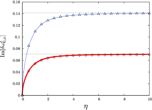
Figure 1: The eigenvalue $\delta\omega_{0,x}^{\varepsilon}$ in case of the perturbation potential $\delta V_{\eta}=gn_{c}\eta/\sqrt{\pi}\exp(-\eta^{2}(\alpha x)^{2})$ with a parameter $\eta$ for $\varepsilon=0.01$. The red (bold) and blue (thin) solid lines indicate the analytic results of perturbation calculation for Eq. (61) with $gn_{c}=1$ and $gn_{c}=2$, respectively, and the open diamonds and triangles indicate the numerical results of the BdG equations for $gn_{c}=1$ and $gn_{c}=2$. The two broken lines mean the analytical values in the limit of $\eta\rightarrow\infty$, i.e. Eq. (68), which are $0.0707\cdots$ for $gn_{c}=1$ and $0.1414\cdots$ for $gn_{c}=2$, respectively.

In Fig. 2, we draw a snapshot of the temporal evolution of the soliton, obtained by solving the TDGP equation (1) for $\delta V_{\eta}$. It is seen during the time evolution that the condensate is distorted by the potential $\delta V_{\eta}$ in its vicinity and that accordingly the displacement of the soliton is enhanced.

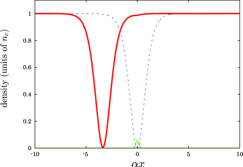
Figure 2: The temporal evolution of the soliton obtained by solving the TDGP equation for the perturbation Gaussian potential $\delta V_{\eta}$ with the parameters $gn_{c}=2$, $\eta=5.0$ and $\varepsilon=0.01$. The blue (broken) line denotes the initial distribution of the soliton whose center is displaced slightly, while the red (solid) one does the distribution after the elapse of a certain time. The shape of the perturbation potential is depicted in green (thin) line.

4.2 Oscillating type potential

Suppose the perturbation potential of

$$\delta V_{k}(x)=gn_{c}\frac{\sin(\alpha kx)}{\tanh(\alpha x)}\left(-3\tanh^{2}(\alpha x)+1-\frac{k^{2}}{2}\right),$$ (69)

with a real parameter $k$. The shape of this potential is shown in Fig. 3. As the parameter $k$ increases, the potential height at $x=0$ where the center of the stationary soliton is initially placed becomes lower.

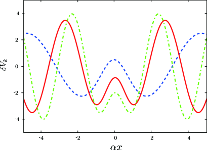
Figure 3: The oscillating type potential $\delta V_{k}(x)$ with the parameter $k=1.0$ (blue broken line), $k=1.73$ (red solid line) and $k=2.0$ (green dashed-dotted line), where $gn_{c}=1$.

The reason why the potential in Eq. (69) is taken is that one can obtain an analytical solution of the first order GP equation, which is

$$\xi^{(1)}(x)=\sqrt{n_{c}}\sin(\alpha kx),\quad\mu^{(1)}=0.$$ (70)

Then $Y^{(xx)}_{0,0}$ is calculated as

$$Y^{(xx)}_{0,0}=2gn_{c}\int ds(1- \tanh^{2}(s))^{2}\frac{\sin(ks)}{\tanh(s)}\left\{3\tanh^{2}(s)+1-\frac{k^{2}}{2}\right\},$$ (71)

where $s=\alpha x$, giving the eigenvalue $\delta\omega_{0,x}^{\varepsilon}$ according to Eq. (61). The result is shown in Fig. 4. There is a critical value of $k$, denoted by $k_{c}=1.73\cdots$, for which $Y^{(xx)}_{0,0}(k_{c})=0$. As $Y^{(xx)}_{0,0}$ is negative for $k>k_{c}$ and positive for $k<k_{c}$, Eq. (61) yields real $\delta\omega_{0,x}^{\varepsilon}$ for $k>k_{c}$ and pure imaginary one for $k<k_{c}$, as is shown in Fig. 4. Note that the sign of $Y^{(xx)}_{0,0}$ depends on $k$ but not on $\alpha=\sqrt{mgn_{c}}$, so $k_{c}$ is independent of $\alpha$. Thus this model exhibits the transition between real and pure imaginary eigenvalues as the parameter $k$ changes continuously.

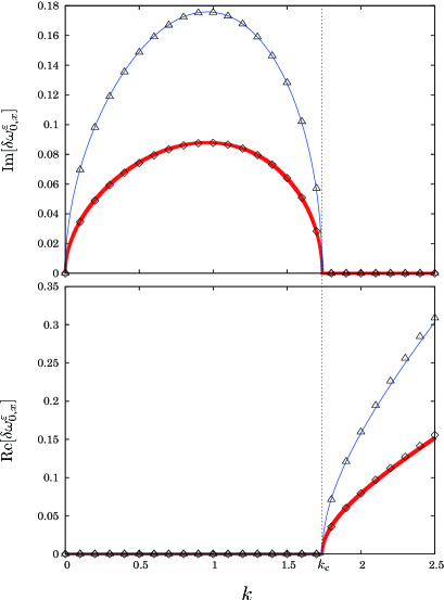
Figure 4: The eigenvalue $\delta\omega_{0,x}^{\varepsilon}$ for the perturbation potential Eq. (69) with the parameter $k$ for $\varepsilon=0.01$. The red (bold) and blue (thin) solid lines indicate the perturbative results Eq.(61) where $gn_{c}=1$ and $gn_{c}=2$, respectively, and the open diamonds and triangles indicate the numerical results of the BdG equations where $gn_{c}=1$ and $gn_{c}=2$. The quantity $k_{c}=1.73\cdots$ is the critical value of the parameter $k$, as is explained in the text.

Similarly as in the previous subsection, it can be checked from the numerical calculation of the TDGP equation that in the region of pure imaginary $\delta\omega_{0,x}^{\varepsilon}$ the dark soliton, displaced very slightly from the center initially, starts to move, and oscillates between the two peaks of the potential, that is, the peak at the center and that next to the center.

5 Summary

In this paper, treating the zero modes for the condensate system properly from the viewpoint of quantum field theory, we have studied possible dynamical instability stemming from the zero modes, and have found eigenfunctions with pure imaginary eigenvalues under a symmetry breaking external perturbation potential. The pure imaginary modes are non-oscillatory, and should cause some exponential blowup of small fluctuation or dynamical instability in accordance with the general arguments of complex modes.

As examples, two one-dimensional homogeneous systems with a dark soliton under perturbation potentials breaking the translational symmetry have been considered. Without the perturbation potentials there appears the $x$-zero mode which is the Nambu-Goldstone one associated with a spontaneous breakdown of the translational symmetry. It is shown that as a result of applying the symmetry breaking potentials it and its adjoint mode can turn into two pure imaginary modes in some cases. In our case of the soliton, the relevant transformation is a translation and the dynamical instability manifests itself such that the center of the soliton moves considerably for its small fluctuation. We have confirmed this, using two types of the perturbation potentials for which analytic solutions are available.

The emergence of the pure imaginary modes stemming from the zero modes provides us with a new scenario of that of the complex modes, other than the degeneracy between excitation modes [11]. Although we treat only single-component BECs for simplicity in this paper, the extension to multi-component BEC [22, 23, 24] is straightforward.

The arguments about the instability in this paper extend only to the c-number solution of the TDGP equation, but not to quantum fluctuations generated by pure imaginary or complex excitation modes. It is desirable to take account of the quantum nature of the pure imaginary modes properly. To do this, we need to resolve the difficulty that the unperturbed Hamiltonian for the pure imaginary mode, $H^{\varepsilon}_{0,{\mathrm{PI}}}$ is not diagonalized and therefore a unique vacuum is not known [17]. Explicitly $H^{\varepsilon}_{0,{\mathrm{PI}}}$ for the one-dimensional soliton model under a symmetry breaking perturbation is given by

$$H^{\varepsilon}_{0,{\mathrm{PI}}}=\delta\omega^{\varepsilon}_{0,x}b^{\dagger}a+\delta\omega^{\varepsilon,\ast}_{0,x}a^{\dagger}b$$ (72)

with the commutation relations for the operators $a$ and $b$, $[a,b^{\dagger}]=1$ and $[a,a^{\dagger}]=[b,b^{\dagger}]=[a,b]=0$ . The diagonalization problem for general complex modes is still open.

In our future work, we will reveal the relation between the dynamical instability in the one-dimensional solitonic system, presented in this paper, and the snake instability in the two or three-dimensional system [21].

References

- [1] M.H. Anderson, J.R. Ensher, M.R. Matthews, C.E. Wieman, and E.A. Cornell, Science 269 (1995) 198.
- [2] K.B. Davis, M.-O. Mewes, M.R. Andrews, N.J. van Druten, D.S. Durfee, D.M. Kurn, and W. Ketterle, Phys. Rev. Lett. 75 (1995) 3969.
- [3] C.C. Bradley, C.A. Sackett, J.J. Tollett, and R.G. Hulet, Phys. Rev. Lett. 75 (1995) 1687.
- [4] Y. Shin, M. Saba, M. Vengalattore, T.A. Pasquini, C. Sanner, A.E. Leanhardt, M. Prentiss, D.E. Pritchard, W. Ketterle, Phys. Rev. Lett. 93 (2004) 160406.
- [5] L. Fallani, L. De Sarlo, J.E. Lye, M. Modugno, R. Saers, C. Fort, and M. Inguscio Phys. Rev. Lett. 93 (2004) 140406.
- [6] L. Khaykovich, F. Schreck, G. Ferrari, T. Bourdel, J. Cubizolles, L.D. Carr, Y. Castin and C. Salomon, Science 296 (2002) 1290.
- [7] N.N. Bogoliubov, J. Phys. (Moscow) 11 (1947) 23.
- [8] P.G. de Gennes, Superconductivity of Metals and Alloys (Benjamin, New York, 1966).
- [9] A.L. Fetter, Ann. of Phys. 70 (1972) 67.
- [10] F. Dalfovo, S. Giorgini, L.P. Pitaevskii and S. Stringari, Rev. Mod. Phys. 71 (1999) 463.
- [11] Y. Nakamura, M. Mine, M.Okumura, and Y. Yamanaka, Phys. Rev. A 77 (2008) 043601.
- [12] Y. Nambu and G. Jona-Lasinio, Phys. Rev. 122 (1961) 345.
- [13] M. Lewenstein and L. You, Phys. Rev. Lett. 77 (1996) 3489.
- [14] H. Matsumoto and S. Sakamoto, Prog. Theor. Phys. 107 (2002) 679.
- [15] J. Dziarmaga, Phys. Rev. A 70 (2004) 063616.
- [16] K. Kobayashi, Y. Nakamura, M. Mine, and Y. Yamanaka, Ann. Phys. 324 (2009) 2359.
- [17] M. Mine, M.Okumura, T. Sunaga, and Y. Yamanaka, Ann. Phys. 322 (2007) 2327.
- [18] J. Dziarmaga and K. Sacha, Phys. Rev. A 66 (2002) 043620.
- [19] R. Ichihara, I. Danshita and T. Nikuni, Phys. Rev. A 78 (2008) 063604.
- [20] S. Middelkamp, G. Theocharis, P.G. Kevrekidis, D.J. Frantzeskakis, and P. Schmelcher, Phys. Rev. A 81 (2010) 053618.
- [21] D.J. Frantzeskakis, J. Phys. A: Math. Theor. 43 (2010) 213001.
- [22] S. Yi, O. E. Mustecaplioglu, and L. You, Phys. Rev. Lett. 90 (2003) 140404.
- [23] S. Yi, O. E. Mustecaplioglu, and L. You, Phys. Rev. A. 68 (2003) 013613.
- [24] Y. Kawaguchi, Phys. Rev. A. 89 (2014) 033627.