ASYMPTOTIC SOLUTIONS FOR MEAN-FIELD SLAB DYNAMOS

Abstract

We discuss asymptotic solutions of the kinematic $\alpha\omega$-dynamo in a thin disc (slab) surrounded by an electric insulator. Focusing upon the strong dynamo regime, in which the dynamo number $D$ satisfies $|D|\gg 1$, we resolve uncertainties in the earlier treatments and conclude that some of the simplifications that have been made in previous studies are questionable. Having abandoned these simplifications, we show, by comparing numerical solutions with complementary asymptotic results obtained for $|D|\gg 1$ and $|D|\ll 1$, that the asymptotic solutions give a reasonably accurate description of the dynamo even far beyond their formal ranges of applicability. Indeed, our results suggest a simple analytical expression for the growth rate of the mean magnetic field that remains accurate across the wide range of values for $D$ that are typical of spiral galaxies and accretion discs. Finally, we analyse the role of various terms in the governing equations to clarify the fine details of the dynamo process. In particular, in the case of the radial magnetic field equation we have shown that the $\alpha\,\upartial B_{\phi}/\upartial z$ term (where $B_{\phi}$ is the azimuthal magnetic field, $\alpha$ is the mean-field dynamo coefficient, and $z$ is measured across the slab), which is neglected in some of the earlier asymptotic studies, is essential for the dynamo as it drives a flux of magnetic energy away from the dynamo region, towards the surface of the slab.

1 Introduction

Mean-field slab (or thin disc) dynamos can be represented by a very simple system of equations, with $z$ (the distance across the slab, parallel to the rotation axis) as the only spatial variable. In the case of astrophysical discs, it is usually appropriate to work with the $\alpha\omega$-dynamo equations, in which it is assumed that the mean inductive effects of the rotational shear (the $\omega$-effect) are significantly stronger than those due to the effects of helical turbulence (the $\alpha$-effect). In systems of this type, the behaviour of the dynamo depends upon the spatial distribution of the $\alpha$-effect across the slab $\alpha(z)$, as well as the imposed boundary conditions and the assumed differential rotation profile. However, once these features have been specified, the $\alpha\omega$-dynamo only has a single control parameter, the dynamo number $D$, which measures the efficiency of the source terms in the dynamo equations relative to magnetic diffusion. Given the importance of the slab dynamos for applications (e.g., galactic and accretion discs), they have attracted a significant amount of attention (e.g., Moffatt, 1978; Parker, 1979; Ruzmaikin et al., 1979, 1988; Beck et al., 1996; Shukurov, 2007; Shukurov and Sokoloff, 2008). The simple structure of their eigensolutions, with a discrete spectrum of real eigenvalues under conditions typical of spiral galaxies and accretion discs, makes this system attractively accessible to analysis.

Exact solutions are known for kinematic $\alpha\omega$ slab dynamos with a few artificial (discontinuous) forms of $\alpha(z)$. Examples include a piecewise constant distribution $\alpha(z)=\alpha_{0}$ for $z>0$, $-\alpha_{0}$ for $z<0$ and $0$ for $z=0$ (Parker, 1979), and a distribution consisting of two delta functions, $\alpha(z)=\alpha_{0}[\delta(z-z_{0})-\delta(z+z_{0})]$, with $\alpha_{0}=\mathrm{const}$ (Moffatt, 1978; Ruzmaikin et al., 1979). These functional forms for $\alpha(z)$ produce both oscillatory and non-oscillatory solutions. However, numerical solutions with continuous $\alpha(z)$ are non-oscillatory for negative dynamo numbers of a moderate magnitude (Ruzmaikin et al., 1980; Stepinski and Levy, 1990). A deeper insight into the nature of the eigensolutions and their dependence upon the distribution of $\alpha(z)$ has been provided by approximate and asymptotic solutions.

Isakov et al. (1981) developed boundary-layer asymptotics for an $\alpha\omega$-dynamo in a slab for $|D|\gg 1$. Adopting a definition for the dynamo number that is consistent with that given below (see equation (5)), these authors were able to show that the growth rate of the leading mode, which has quadrupolar parity, has the form

$$\gamma\simeq\bar{\gamma}_{0}\left|\alpha^{\prime}(0)D\right|^{1/2}\,,$$ (1)

where $\alpha^{\prime}(0)$ is the value of $\mathrm{d}\alpha/\mathrm{d}z$ at $z=0$ and $\bar{\gamma}_{0}$ is a constant of order unity. In their study, this constant was determined to be $\bar{\gamma}_{0}\approx 0.3$ from fitting this form to a numerical solution. These authors used further simplifications to reduce the problem to a second-order ordinary differential equation which still is not amenable to analytic solution. We discuss and assess these simplifications below (see also Appendix 6, where we show, in particular, that the simplified asymptotic boundary value problem considered by these authors in fact has only trivial quadrupolar solutions for $D<0$). Following Isakov et al. (1981), Sokoloff (1995) similarly simplified the $\alpha\omega$-dynamo equations to obtain, from a WKB asymptotic solution, $\gamma\simeq\left|\alpha^{\prime}(0)D\right|^{1/2}$. It remains unclear how these asymptotic solutions are related to each other, how they compare to the numerical ones, and what their ranges of applicability are.

In this paper, we revisit the asymptotic solutions of the kinematic $\alpha\omega$-dynamo in a slab. We discuss the various approximations involved and resolve some earlier uncertainties to present what is arguably a definitive asymptotic analysis for $|D|\gg 1$. These asymptotics are then compared with both numerical solutions and analytical results from perturbation theory (formally applicable for $|D|\ll 1$). We demonstrate that both asymptotic solutions, for $|D|\gg 1$ and $|D|\ll 1$, remain remarkably accurate far beyond their formal ranges of applicability. Thus, solutions obtained and discussed here offer a firm foundation for further qualitative studies and applications to galactic and accretion-disc dynamos. Having presented the dynamo equations in section 2, we discuss in section 3 the form of their asymptotic solutions in the kinematic regime, i.e., when the back-reaction of magnetic fields on the velocity field is still negligible and the magnetic field strength grows exponentially with time. Numerical solutions for the slab $\alpha\omega$-dynamo surrounded by a vacuum are presented in section 4, and then compared to the asymptotic solutions for both $|D|\gg 1$ and $|D|\ll 1$. This clarifies the applicability of various assumptions employed in deriving the asymptotic solutions and allows us to establish their final form. The implications of our results are discussed in section 5. Various simplifications and their pitfalls are discussed in Appendix 6.

2 Disc dynamos

The evolution of a large-scale magnetic field $\bm{B}$ in an electrically conducting fluid is governed by the mean-field dynamo equation (e.g., Moffatt, 1978; Krause and Rädler, 1980)

$$\frac{\upartial\bm{B}}{\upartial t}=\bm{\nabla}\times(\bm{V}\times\bm{B})+\bm{\nabla}\times(\alpha\bm{B})-\eta\bm{\nabla}\times\bm{\nabla}\times\bm{B},$$ (2)

where $\alpha$ represents the mean-field $\alpha$-effect (production of the mean magnetic field by a mirror-asymmetric random flow), $\bm{V}$ is the large-scale fluid velocity and $\eta$ is the magnetic diffusivity (usually dominated by its turbulent part) which is assumed, for simplicity, to be independent of position. In the framework of the kinematic dynamo theory, $\bm{V}$ and $\alpha$ are prescribed functions of position, and are thus independent of $\bm{B}$.

We introduce cylindrical polar coordinates $(r,\phi,z)$ with the origin at the disc centre and the $z$-axis perpendicular to the disc (or slab) plane. The disc is assumed to have a horizontal size $L$ and thickness $2h$. We restrict our attention to axisymmetric solutions of equation (2) and assume that $L\gg h$, meaning that the disc is thin. The advantage of considering the thin disc limit is that the terms involving radial derivatives (and those in $\phi$) are much smaller than those with derivatives in $z$, and can therefore be neglected in the lowest approximation (Ruzmaikin et al., 1988). In most astrophysical applications, the large-scale velocity field is dominated by an overall rotation and, thus, is predominantly azimuthal. Since $\upartial V/\upartial z\approx 0$ at $z\approx 0$ from symmetry considerations, the large-scale velocity field in a thin layer is practically independent of $z$. We can therefore assume that the large-scale velocity field takes the form $\bm{V}(r)=(0,r\varOmega(r),0)$.As $\varOmega$ decreases with $r$ in most cases of interest, we can also assume that $\mathrm{d}\varOmega/\mathrm{d}r<0$. The rotational velocity shear rate is given by $G(r)=r\,\mathrm{d}\varOmega/\mathrm{d}r$, which will be assumed to be constant in this study, $G(r)=G_{0}$, with $G_{0}<0$. In a thin layer, the evolution equation for $B_{z}$ decouples from the equations for $B_{r}$ and $B_{\phi}$, so only the latter two equations must be considered in the subsequent analysis. Once these equations have been solved, it is straightforward to calculate $B_{z}$ using the fact that $\bm{\nabla}\cdot\bm{B}=0$ (Ruzmaikin et al., 1988).

Dimensionless variables, denoted with a circumflex, can be conveniently defined as follows:

$$t=\frac{h^{2}}{\eta}\widehat{t}\,,\quad r=L\widehat{r}\,,\quad z=h\widehat{z}\,,\quad B_{r}=B_{0}\widehat{B_{r}}\,,\quad B_{\phi}=\frac{B_{0}\eta}{h\alpha_{0}}\widehat{B_{\phi}}\,,\quad\alpha=\alpha_{0}\widehat{\alpha}\,,$$

where $B_{0}$ and $\alpha_{0}$ are representative values of the magnetic field and $\alpha$-effect, respectively. Throughout the remainder of this paper, all variables will be dimensionless unless stated otherwise. So, to simplify notation, we drop the circumflex in what follows. Having introduced these scalings, we are left with the following dimensionless equations for the magnetic field components $B_{r}$ and $B_{\phi}$:

$$\frac{\upartial{B}_{r}}{\upartial t} = -\frac{\upartial}{\upartial z}(\alpha B_{\phi})+\frac{\upartial^{2}B_{r}}{\upartial z^{2}}\,,$$ (3)

$$\frac{\upartial{B}_{\phi}}{\upartial t} = DB_{r}+\frac{\upartial^{2}B_{\phi}}{\upartial z^{2}}\,,$$ (4)

where

$$D=\frac{\alpha_{0}G_{0}h^{3}}{\eta^{2}}$$ (5)

is the dynamo number; $|D|$ must exceed a certain critical value $|D_{\mathrm{cr}}|$ to allow magnetic field to grow.

As the velocity field is independent of $\bm{B}$, solutions have the form

$$\bm{B}(z,t)=\bm{b}(z)\mathrm{e}^{\gamma t}\,,$$

leading to

$$\gamma b_{r} = -\frac{\mathrm{d}}{\mathrm{d}z}(\alpha b_{\phi})+\frac{{\mathrm{d}^{2}}b_{r}}{\mathrm{d}z^{2}}\,,$$ (6)

$$\gamma b_{\phi} = Db_{r}+\frac{{\mathrm{d}^{2}}b_{\phi}}{\mathrm{d}z^{2}}\,.$$ (7)

From the overall symmetry of the problem, $\alpha$ is an odd function of $z$, which implies that $\alpha(z)=-\alpha(-z)$ with $\alpha(z)>0$ for $z>0$ (Ruzmaikin et al., 1988). As a consequence of this the solutions are either quadrupolar [with $b_{r,\phi}(-z)=b_{r,\phi}(z)$ and $b_{z}(-z)=-b_{z}(z)$] or dipolar [with $b_{r,\phi}(-z)=-b_{r,\phi}(z)$ and $b_{z}(-z)=b_{z}(z)$]. Earlier results demonstrate that quadrupolar modes dominate strongly in a thin layer surrounded by an electric insulator (vacuum) (Moffatt, 1978; Ruzmaikin et al., 1988). Therefore, we consider the range $0\leq z\leq 1$ and apply the following boundary conditions at the disc mid-plane that respect the quadrupolar symmetry:

$$\frac{\mathrm{d}b_{r}}{\mathrm{d}z}=\frac{\mathrm{d}b_{\phi}}{\mathrm{d}z}=0\quad\mbox{at}\ z=0.$$ (8)

At the surface of the layer, $z=1$, we adopt the vacuum boundary conditions (Moffatt, 1978; Ruzmaikin et al., 1988),

$$b_{r}=b_{\phi}=0\quad\mbox{at}\ z=1\,.$$ (9)

An eigenvalue problem has now been formulated, with $\gamma$ the eigenvalue, $(b_{r},b_{\phi})$ the eigenfunction and $D$ the control parameter. The solution obviously depends upon the spatial distribution of $\alpha(z)$. However, this dependence is not strong. For example, regardless of the choice for $\alpha(z)$, it is rare for the critical dynamo number to lie outside of the narrow range $-13\leq D_{\mathrm{cr}}\leq-4$ (Ruzmaikin et al., 1988), even with a discontinuous distribution for the $\alpha$-effect.

3 Boundary layer produced by strong dynamo action

In the outer parts of spiral galaxies, $\left|D\right|\sim 10$, whilst values of a few hundred are typical of their central regions (e.g., Shukurov, 2007). It is therefore reasonable to look for asymptotic solutions for large dynamo number, $\left|D\right|\gg 1$. As discussed here, for large $|D|$ a boundary layer develops at $z\approx 0$.

In this analysis, we consider smooth functional forms for the $\alpha$-effect. Since $\alpha(z)$ is an odd function, it can be expanded as $\alpha(z)\approx\alpha_{1}z+\alpha_{3}z^{3}+...$ in the vicinity of $z=0$ (where $\alpha_{1}$ and $\alpha_{3}$ are dimensionless constants of order unity). The special case of $\alpha_{1}=0$ is discussed briefly below. However, unless stated otherwise, we shall assume that $\alpha_{1}$ is strictly positive throughout this section. In this case, we can further assume (without loss of generality) that $\alpha_{1}=1$ because we are free to choose an appropriate scaling for the $\alpha$-effect when the equations are made dimensionless. So, at leading order, $\alpha(z)\approx z$ in the vicinity of $z=0$.

We introduce the scaled variable,

$$s=|D|^{k}z\,,$$

and assume the following scalings within the boundary layer:

$$\frac{\mathrm{d}}{\mathrm{d}z}=|D|^{k}\frac{\mathrm{d}}{\mathrm{d}s}\,,\qquad b_{r}=\left|D\right|^{n}R(s)\,,\qquad b_{\phi}=\varPhi(s)\,,\qquad\gamma=\varGamma_{0}|D|^{m}\,,$$

where $k$, $m$ and $n$ must be determined. Having written the term responsible for the $\alpha$-effect in equation (6) as

$$\frac{\mathrm{d}}{\mathrm{d}z}(\alpha b_{\phi})=\frac{\mathrm{d}\alpha}{\mathrm{d}z}b_{\phi}+\alpha\frac{\mathrm{d}b_{\phi}}{\mathrm{d}z}\,,$$ (10)

we note that, within the boundary layer,

$$\frac{\mathrm{d}\alpha}{\mathrm{d}z}b_{\phi}\approx\varPhi(s)=\mathrm{O}(1)\,,$$

and

$$\alpha\frac{\mathrm{d}b_{\phi}}{\mathrm{d}z}\approx z\frac{\mathrm{d}b_{\phi}}{\mathrm{d}z}=s\frac{\mathrm{d}\varPhi}{\mathrm{d}s}=\mathrm{O}(1)\,.$$

Thus, the two terms in $\mathrm{d}(\alpha b_{\phi})/\mathrm{d}z$ are of the same order of magnitude in $\left|D\right|$ and neither of them can be neglected. It is straightforward to show that this is also the case when $\alpha_{1}=0$ (i.e., $\alpha=\alpha_{3}z^{3}+\ldots$). Although quadrupolar solutions tend to be preferred in this disc dynamo system, it can be shown that these terms would also be of the same order of magnitude if dipolar boundary conditions had been adopted, so this is a very general result.

For these quadrupolar solutions, all of the terms in equations (6) and (7) are of the same order of magnitude in $|D|$ if

$$k=1/4,\quad m=1/2,\quad n=-1/2.$$

Then the governing equations reduce to

$$\varGamma_{0}R = -\frac{\mathrm{d}}{\mathrm{d}s}(s\varPhi)+\frac{\mathrm{d}^{2}R}{\mathrm{d}s^{2}}\,,$$ (11)

$$\varGamma_{0}\varPhi = \mbox{sign}(D)\,R+\frac{\mathrm{d}^{2}\varPhi}{\mathrm{d}s^{2}}\,,$$ (12)

$$\frac{\mathrm{d}R}{\mathrm{d}s} (0) =\frac{\mathrm{d}\varPhi}{\mathrm{d}s}(0)=0\,,\quad|R|,|\varPhi|\rightarrow 0\ \mbox{as}\ s\rightarrow\infty\,.$$ (13)

These boundary-layer equations are no simpler to solve than the original ones. This fact has prompted earlier authors to neglect $s\,\mathrm{d}\varPhi/\mathrm{d}s$ in the first equation. It is now clear that this is unacceptable in any physically justifiable case. More details regarding possible simplifications can be found in Appendix 6.

Useful results can be obtained even from the form of the asymptotic solutions now clarified. In particular, we have shown that $\displaystyle{b_{\phi}/b_{r}}$ and $\gamma$ are both $\displaystyle{\mathrm{O}(\left|D\right|^{1/2})}$ quantities in this asymptotic regime [cf. equation (1)], whilst the magnetic field eigenfunctions vary over a characteristic spatial scale $\displaystyle{\mathrm{O}(\left|D\right|^{-1/4})}$. These quantitative predictions can be tested numerically and used in applications. Isakov et al. (1981) obtained similar scalings but their further analysis involved a strong assumption that $|R(s)|\propto|\varPhi(s)|$. This assumption is not supported by the numerical solutions reported in section 4.

Similar boundary-layer equations can be derived in the case $\alpha_{1}=0$. If the first non-zero term of the Taylor-series expansion for $\alpha(z)$ is $\alpha_{p}z^{p}$ (with $\alpha_{p}>0$), all of the terms in the governing equations contribute at the same order in $\left|D\right|$ if $\displaystyle{m=2/(p+3),\;n=-(p+1)/(p+3)}$ and $\displaystyle{k=1/(p+3)}$.

We should make one final comment before proceeding. As stressed by Sokoloff (1995), the asymptotic solutions discussed here are of intermediate nature as they apply when, on the one hand, $|D|\gg 1$ but, on the other hand, when $|D|$ is not too large. For $D\mathrel{\mathchoice{\vbox{\offinterlineskip\halign{\hfil$\displaystyle#$\hfil\cr<\cr\sim\cr}}}{\vbox{\offinterlineskip\halign{\hfil$\textstyle#$\hfil\cr<\cr\sim\cr}}}{\vbox{\offinterlineskip\halign{\hfil$\scriptstyle#$\hfil\cr<\cr\sim\cr}}}{\vbox{\offinterlineskip\halign{\hfil$\scriptscriptstyle#$\hfil\cr<\cr\sim\cr}}}}-300$, the leading eigenvalue can be complex and dipolar modes can become dominant. Under these circumstances, these solutions will no longer be valid. However, these parameter regimes are arguably less relevant for galactic applications.

4 Numerical solutions

In order to clarify the nature of the asymptotic solutions and to assess the validity of various approximations, we solved numerically for the leading eigensolution of equations (3) and (4), adopting the quadrupolar symmetry conditions (8) and vacuum boundary conditions (9) written for $B_{r}$ and $B_{\phi}$. We also assume here that

$$\alpha=\sin\pi z\,,$$

so that $\alpha_{1}=\pi$. In addition, following Isakov et al. (1981), we shall obtain an accurate value of the constant $\bar{\gamma}_{0}$ in the asymptotic expression (1) for the eigenvalue. We used a fourth-order Runge–Kutta time stepping scheme, adopting a second-order finite difference approximation for the spatial derivatives (including the boundary conditions). All calculations made use of $N=100$ mesh points in $0\leq z\leq 1$. This numerical resolution is more than adequate for the values of $D$ that have been considered.

The growth rate $\gamma$ of the magnetic field, for various values of the dynamo number $D$, for the leading quadrupole mode. The upper table shows our results, which were obtained using $N=100$ mesh points in $0\leq z\leq 1$, whilst the lower part of the table shows the results with $N=10$ from Ruzmaikin et al. (1980). The entries in the lower part of the table should be compared with the bold entries in the upper part of the table. $N=100$ $D$ $-5$ $-8$ $-10$ $-12$ $-15$ $-20$ $-25$ $\gamma$ $\mathbf{-0.50}$ $\mathbf{0.00}$ $\mathbf{0.27}$ $0.52$ $0.85$ $\mathbf{1.33}$ $1.73$ $D$ $-30$ $-35$ $-40$ $-50$ $-60$ $-70$ $-80$ $\gamma$ $2.09$ $2.41$ $2.70$ $\mathbf{3.20}$ $3.64$ $4.01$ $4.34$ $D$ $-90$ $-100$ $-120$ $-140$ $-160$ $-180$ $-190$ $\gamma$ $4.63$ $\mathbf{4.88}$ $5.30$ $5.62$ $5.85$ $6.00$ $6.04$ $D$ $-200$ $-205$ $-210$ $-220$ $-250$ $-270$ $-300$ $\gamma$ $6.07$ $6.08$ $6.07$ $6.06$ $5.88$ $5.62$ $\mathbf{4.87}$      $N=10$ $D$ $-5$ $-8$ $-10$ $-20$ $-50$ $-100$ $-300$ $\gamma$ $-0.5$ $-0.0$ $0.3$ $1.4$ $3.4$ $5.2$ $5.6$

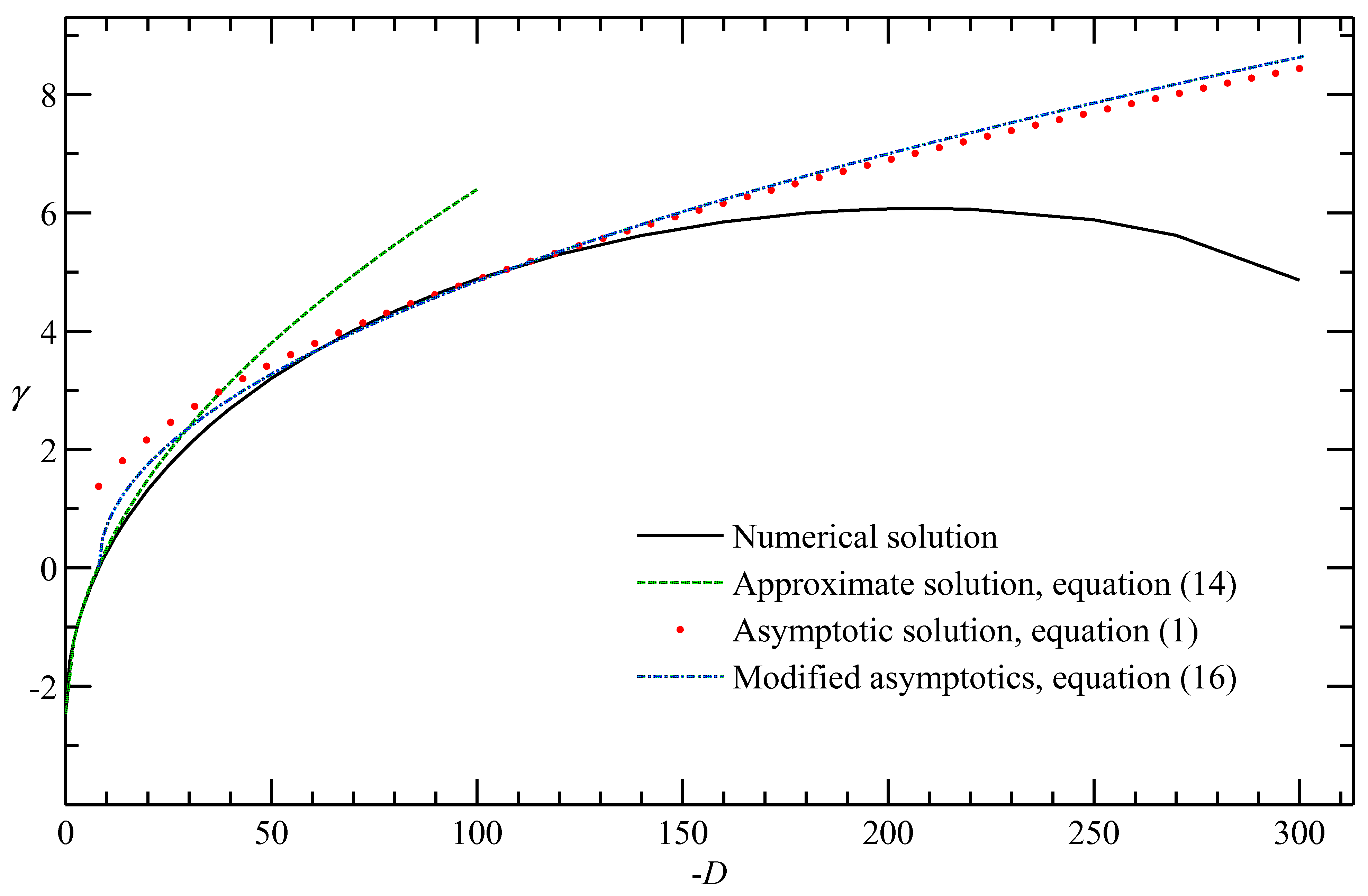
Figure 1: The dependence of the growth rate of the magnetic field on the dynamo number, with numerical results being compared to various approximations. The lines show the numerical solution with $\alpha=\sin\pi z$ (black, solid), the asymptotic solution (1) for $|D|\gg 1$ with $\bar{\gamma_{0}}=0.275$ (red, dotted), the perturbation solution (14) for $|D|\ll 1$ (green, dashed), and the modified asymptotic form (16) for $|D|\gg 1$ with $\alpha^{\prime}(0)=\pi$ (blue, dash-dotted).

Focusing entirely upon negative values of the dynamo number ($-5\geq D\geq-300$), we present in Table 4 the dynamo growth rate $\gamma$ for a range of $D$, and compare it with the earlier results of Ruzmaikin et al. (1980) (which were obtained at a lower numerical resolution). For all dynamo numbers in this range, the solutions are (as expected) non-oscillatory, with the magnetic field growing for $D<D_{\mathrm{cr}}\approx-8$. Despite significant differences in the numerical resolution, the results compare favourably with those of Ruzmaikin et al. (1980) for small values of $|D|$ (see also Stepinski and Levy, 1990). At larger values of $|D|$, we observe a local maximum in the growth rate, with $\gamma$ reaching a peak value at $D\approx-205$. The growth rate of the non-oscillatory quadrupolar mode then decreases for larger values of $|D|$.

4.1 The growth rate of the magnetic field

The dependence of the growth rate of the magnetic field upon the dynamo number is shown in figure 1. For small values of $|D|$, these results compare very favourably to the corresponding perturbation solution (for this choice of $\alpha=\sin\pi z$) of Shukurov and Sokoloff (2008),

$$\gamma=-\tfrac{1}{4}\pi^{2}+\tfrac{1}{2}\sqrt{-\pi D}+\mathrm{O}(|D|^{3/2})\,,\qquad\alpha=\sin\pi z\,,\qquad|D|\ll 1\,.$$ (14)

This result is only weakly dependent upon the choice of functional form for $\alpha(z)$. For example, for $\alpha=z$, we have for the leading quadrupolar mode

$$\gamma=-\tfrac{1}{4}\pi^{2}+\sqrt{-\tfrac{1}{2}D}+\mathrm{O}(|D|^{3/2})\,,\qquad\alpha=z\,,\qquad|D|\ll 1\,,$$

where the factor in front of $\sqrt{-D}$ differs from that in equation (14) by 25%, leading to $D_{\mathrm{cr}}\approx-12$ instead of $-8$. This difference is arguably negligible given the uncertainties and scatter of galactic parameters as well as other idealisations adopted in the dynamo model. Since the asymptotics for $|D|\gg 1$ are even less sensitive to the form of $\alpha(z)$ away from the boundary layer near $z=0$, we conclude that the results obtained with $\alpha=\sin\pi z$ are representative of the solutions obtained with any other reasonable specific form of $\alpha(z)$.

At larger values of $|D|$, we see that there is a range of dynamo numbers, $-60\geq D\geq-160$, over which the growth rate obtained numerically can be well approximated by a power law in $D$. Applying linear regression, we obtain the following approximation in this range:

$$\gamma\approx 0.44\left|D\right|^{0.52}\,.$$ (15)

Comparing this expression with equation (1) we see that these are comparable if $\bar{\gamma_{0}}\approx 0.275$, which is similar to the value found by Isakov et al. (1981). The accuracy, and usefulness for applications, of the asymptotic solution for $|D|\gg 1$ can be enhanced by replacing $D$ by $D-D_{\mathrm{cr}}$ with $D_{\mathrm{cr}}=-8$ in equation (1); the resulting dependence,

$$\gamma\approx 0.275\left[\alpha^{\prime}(0)(D_{\mathrm{cr}}-D)\right]^{1/2}\,,\qquad D_{\mathrm{cr}}=-8,\quad-160\mathrel{\mathchoice{\vbox{\offinterlineskip\halign{\hfil$\displaystyle#$\hfil\cr<\cr\sim\cr}}}{\vbox{\offinterlineskip\halign{\hfil$\textstyle#$\hfil\cr<\cr\sim\cr}}}{\vbox{\offinterlineskip\halign{\hfil$\scriptstyle#$\hfil\cr<\cr\sim\cr}}}{\vbox{\offinterlineskip\halign{\hfil$\scriptscriptstyle#$\hfil\cr<\cr\sim\cr}}}}D<D_{\mathrm{cr}}\,,$$ (16)

is also shown in figure 1.

The degree of agreement between the two approximations is striking. Most notably, the growth rate predictions for $|D|\ll 1$ and $|D|\gg 1$ evidently remain reasonably accurate even far beyond their respective ranges of applicability. Such behaviour is not unusual in asymptotic solutions; in our case, it apparently results from the simple form of the eigenfunction (see below), as well as from the similarity of the scalings of $\gamma$ with $|D|^{1/2}$ in both asymptotic extremities.

4.2 The eigenfunctions

Figure 2: The eigenfunctions $b_{r}$ (dashed) and $b_{\phi}$ (solid), normalised to $b_{\phi}=1$ at $z=0$, for $D=-20,\ -50,\ -100,\ -150,\ -200$ and $-300$. Solutions become concentrated near the slab mid-plane, $z=0$, as the dynamo number increases in magnitude. The radial magnetic field component $b_{r}$ always changes sign at a certain value of $z$ in any growing solution, whereas $b_{\phi}$ only changes sign for large $\left|D\right|$.

Figure 4.2 shows the eigenfunctions obtained numerically for various values of the dynamo number. For ease of comparison, the eigenfunctions have all been normalised so that $b_{\phi}=1$ at $z=0$. For small values of $|D|$, $b_{\phi}$ decreases monotonically with increasing $z$. However, $b_{r}$ (which is negative at $z=0$) always changes sign at some point within the domain. The value of $z$ at which $b_{r}$ changes sign decreases with increasing $|D|$. Ruzmaikin et al. (1979) have clarified the importance of this feature for the dynamo action: the change of sign of $b_{r}$ drives a diffusive magnetic flux from the dynamo region, thus allowing magnetic field to grow. For larger values of $|D|$, there is also a sign change in $b_{\phi}$, although this always occurs at a larger value of $z$ than the zero of $b_{r}$. Notably, the non-monotonic behaviour of $b_{\phi}$ becomes pronounced for $D\leq-150$ when the dependence of $\gamma$ on $|D|$ deviates from a power law. This signifies a progressive reduction in the accuracy of the asymptotic solution, (15) or (16), as $|D|$ increases further.

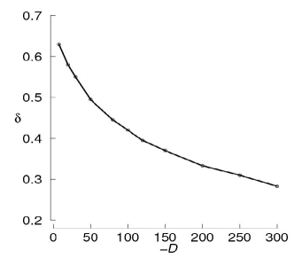
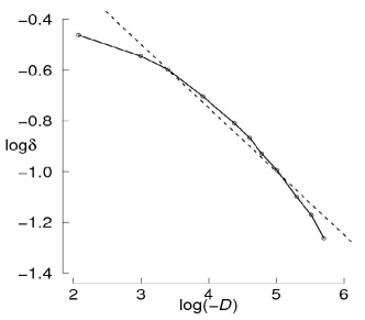
Figure 3: Left panel: The half-width at half-maximum of the eigenfunction, $\delta$, as a function of $|D|$. Right panel: The corresponding linear regression of $\ln\delta$ versus $\ln\left|D\right|$, $\ln\delta\approx-0.2387\ln|D|+0.2079$ for $-160\leq D\leq-60$, with the asymptotic result shown dashed

.

Conforming to the concept of a boundary layer at $|D|\gg 1$, the eigenfunction becomes more concentrated near the slab mid-plane as $|D|$ increases, so the scale in $z$, on which these functions vary, becomes smaller at larger dynamo numbers. This can be quantified in terms of $\delta$, the half-width at half-maximum of $b_{\phi}$:

$$b_{\phi}(\delta)=\tfrac{1}{2}b_{\phi}(0)=\tfrac{1}{2}\,.$$

Figure 3 shows the $D$-dependence of $\delta$ obtained numerically. The linear-regression fit of a power law has the form

$$\delta\approx 1.2\,\left|D\right|^{-0.24}\,,\quad-160\leq D<-60\,.$$

This scaling is consistent with the asymptotic analysis, which suggests that the scale of the eigenfunction varies as $|D|^{-1/4}$.

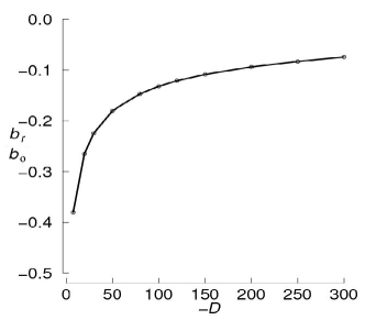
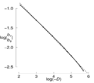
Figure 4: Left panel: The ratio $b_{r}/b_{\phi}$ at $z=0$, as a function of $-D$ for $D<0$. Right panel: The approximation obtained by linear regression, $\ln|b_{r}/b_{\phi}|\approx-0.461\ln\left|D\right|+0.0797$ at $z=0$, with the asymptotic result shown dashed

.

The magnetic pitch angle $p_{B}$, defined as $p_{B}=\arctan|b_{r}/b_{\phi}|$, is a readily observable quantity in galaxies, and it has been shown to be a sensitive diagnostic of the galactic dynamo action (e.g., Shukurov, 2007). Figure 4 shows the related quantity, $b_{r}/b_{\phi}$ evaluated at $z=0$. Its dependence on $D$ is very well approximated by a power law,

$$\frac{b_{r}}{b_{\phi}}\approx-1.1\,|D|^{-0.46}\,,\quad-160\leq D<-60\,.$$

Again, the numerical results agree well with the asymptotic scaling $b_{r}/b_{\phi}\propto|D|^{-1/2}$.

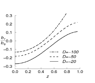
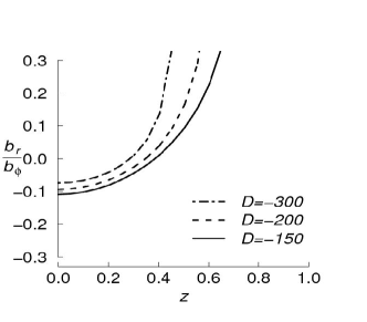
Figure 5: The ratio $b_{r}/b_{\phi}$ as a function of $z$ for $D=-20$,$-50$ and $-100$ (left-hand panel) and $D=-150$, $-200$ and $-300$ (right-hand panel), with line styles indicated in the figure legends.

In their analytic study, Isakov et al. (1981) assumed that the eigenfunctions of $b_{\phi}$ and $b_{r}$ differed only by a constant of proportionality. This assumption allowed these authors to reduce the problem to a single ordinary differential equation. To clarify whether such an assumption is justifiable, we show in figure 5 the ratio $b_{r}/b_{\phi}$ as a function of $z$. For the assumption $b_{r}/b_{\phi}=\mbox{const}$ to be valid, the relative change in this ratio should not exceed $\mathrm{O}(|D|^{-1/4})$ within the boundary layer. The relative change in $b_{r}/b_{\phi}$ is 0.46, 0.48 and 0.40 at $D=-50,-150$ and $-300$ even within a single length scale, $0\leq z\leq|D|^{-1/4}$, with $|D|^{-1/4}=0.38,0.29$ and $0.24$, respectively. Thus, this assumption is dangerous at least, if applicable at all.

Figure 6: The individual terms representing the $\alpha$-effect, $(\alpha b_{\phi})^{\prime}=\alpha^{\prime}b_{\phi}+\alpha b_{\phi}^{\prime}$, for $\alpha=\sin\pi z$ and $D=-20,\ -50,\ -100,\ -150,\ -200$ and $-300$ (here prime denotes derivative in $z$). The term on the left-hand side of the equation, $(\alpha b_{\phi})^{\prime}$, is shown solid, $\alpha^{\prime}b_{\phi}$, dashed, and $\alpha b_{\phi}^{\prime}$,

dash-dotted. In each case, the curves have been normalised so that $(\alpha b_{\phi})^{\prime}=\pi$ at $z=0$. The contribution from $\alpha^{\prime}b_{\phi}$ dominates near $z=0$ whereas $\alpha b_{\phi}^{\prime}$ dominates at mid-depths.

4.3 The inner working of the dynamo

Finally, we consider the role of the various contributions to the $\alpha$-effect in the dynamo mechanism. One of the main conclusions of the asymptotic analysis was that the two different parts of the $\alpha$-effect on the right-hand side of equation (10) should (in general) be of a comparable magnitude in $|D|$, which means that neither should be neglected. Figure 4.2 shows the spatial dependence of the terms that represent the $\alpha$-effect in the governing equations. Since $\alpha(0)=0$ and $b^{\prime}_{\phi}(0)=0$ , it is unsurprising that $(\alpha b_{\phi})^{\prime}\approx\alpha^{\prime}b_{\phi}$ in the immediate vicinity of $z=0$ (with prime denoting the derivative with respect to $z$). However, $|\alpha^{\prime}b_{\phi}|$ decreases with $z$, with $\alpha b_{\phi}^{\prime}$ making the dominant (negative) contribution to the $\alpha$-effect at larger $z$. This transition occurs at progressively smaller values of $z$ as $|D|$ increases, $(\alpha b_{\phi})^{\prime}=0$ at $z\approx 0.26$ for $D=-150$ and $z\approx 0.2$ for $D=-300$. With the spatial scale of the solution of order $|D|^{-1/4}\approx 0.29$ for $D=-150$ and $0.24$ at $D=-300$, $(\alpha b_{\phi})^{\prime}$ changes sign within the boundary layer. Clearly the neglect of either of these terms would affect the solution.

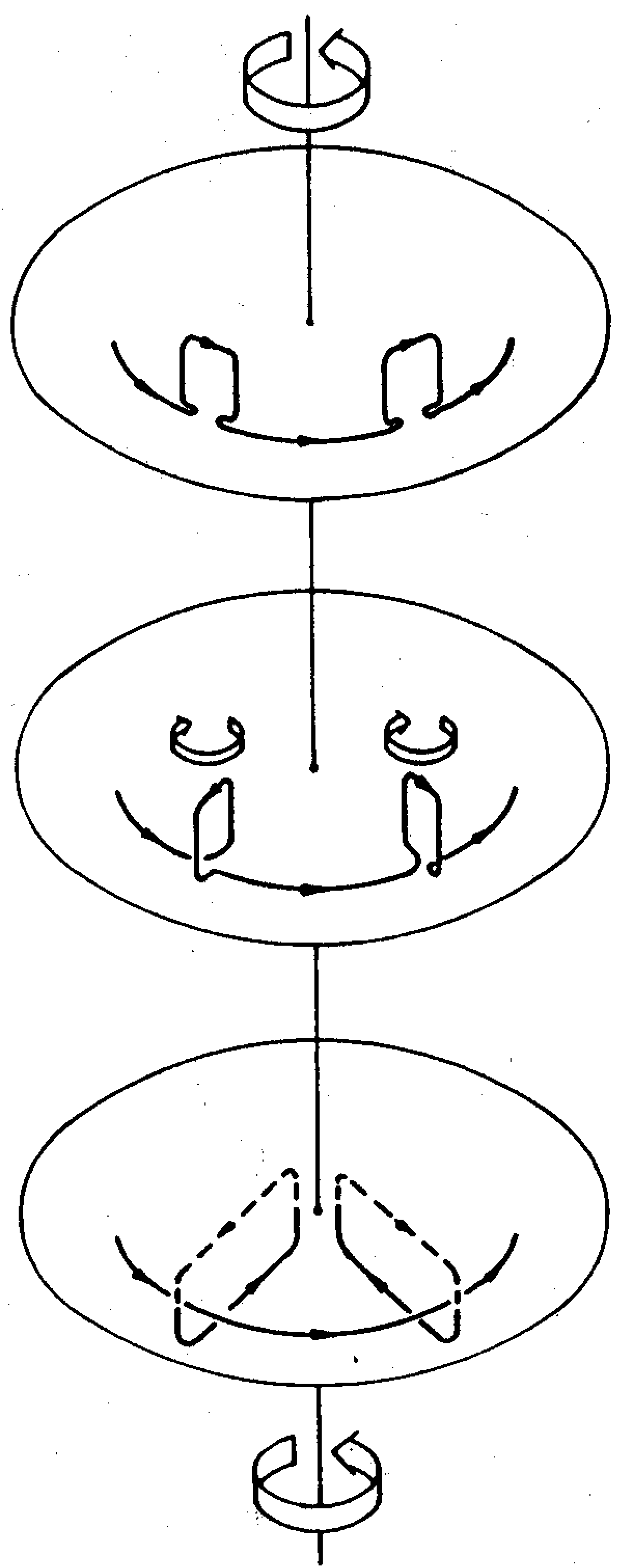
Figure 7: The action of the $\alpha$-effect on the azimuthal magnetic field produces a poloidal field inside the disc by twisting turbulent magnetic loops in a systematic manner. The upper part of the meridional magnetic line (shown dashed in the lowest panel) leaves the disc due to the diffusive flux. Only the upper half-space is shown in all the panels; mirror-antisymmetric events occur in the lower half-space (after Ruzmaikin et al., 1988).

Since $b_{r}<0$, and $\mathrm{d}^{2}b_{r}/\mathrm{d}z^{2}>0$ near $z=0$, it follows from equation (6) that $\gamma>0$ because $(\alpha b_{\phi})^{\prime}>0$ near $z=0$. With $\mathrm{d}b_{r}/\mathrm{d}z>0$, its diffusive flux,$-\mathrm{d}b_{r}/\mathrm{d}z$, is directed towards the midplane. At larger values of $z$, both $(\alpha b_{\phi})^{\prime}$ and $\mathrm{d}^{2}b_{r}/\mathrm{d}z^{2}$ change sign, the former because $\alpha b_{\phi}^{\prime}$ becomes dominant (see figure 4.2), and the latter, due to a change in the curvature of $b_{r}(z)$ (see figure 4.2). Now, $\mathrm{d}b_{r}/\mathrm{d}z<0$ and the diffusive flux of $b_{r}$ is directed out of the dynamo-active region. Ruzmaikin et al. (1979) discuss the importance of the outward flux through the surface (and the change of sign of $b_{r}$ within the slab) for the dynamo action: magnetic field produced by the $\alpha$-effect near the surface of the slab (shown dashed in the lowest panel of figure 7) must leave through its surface to ensure that the oppositely directed net poloidal magnetic field (shown solid) can grow within the slab.

Thus, the term $\alpha b_{\phi}^{\prime}$ opposes the dynamo action by reducing the rate of growth of the radial magnetic field near the mid-plane of the slab. Its role in the dynamo action consists of driving the outward diffusive flux of magnetic field by changing the sign of $b_{r}$ closer to the slab surface. It is clear that such a surface-directed flux must occur within the boundary layer to allow magnetic field to grow, and hence this term cannot be neglected even within the boundary layer. We show in Appendix 6 that the dynamo equations have only trivial solutions for $D<0$ if this term is neglected.

However, driving the flux to the surface comes at a price for the dynamo action. For $D\mathrel{\mathchoice{\vbox{\offinterlineskip\halign{\hfil$\displaystyle#$\hfil\cr<\cr\sim\cr}}}{\vbox{\offinterlineskip\halign{\hfil$\textstyle#$\hfil\cr<\cr\sim\cr}}}{\vbox{\offinterlineskip\halign{\hfil$\scriptstyle#$\hfil\cr<\cr\sim\cr}}}{\vbox{\offinterlineskip\halign{\hfil$\scriptscriptstyle#$\hfil\cr<\cr\sim\cr}}}}-160$, the negative contribution of $\alpha b_{\phi}^{\prime}$ becomes so strong that the dynamo action is affected and $\gamma$ increases with $|D|$ more gradually, and eventually even decreases for $D<-205$, as shown in figure 1. Other modes, which become dominant at still larger values of $|D|$, require a different balance of terms and can prosper.

5 Conclusions and discussion

This study has shown that the asymptotic and perturbation solutions of the mean-field $\alpha\omega$-dynamo are remarkably accurate in a wide range of dynamo numbers that covers those encountered in spiral galaxies and accretion discs near black holes and protostars. This provides a firm basis for the exploration of the origin of large-scale magnetic fields in those objects. We have also clarified the role of various terms in the dynamo equations, especially $\alpha\,\mathrm{d}B_{\phi}/\mathrm{d}z$ and $B_{\phi}\,\mathrm{d}\alpha/\mathrm{d}z$, and demonstrated that neither of these terms should be neglected in a boundary-layer analysis. Indeed, as shown in Appendix 6, the neglect of the $\alpha\,\mathrm{d}B_{\phi}/\mathrm{d}z$ term implies that the boundary-layer equations only have trivial solutions for $D<0$. As emphasized by Sokoloff (1995), the solutions that are considered here are intermediate asymptotics as they apply at $D\ll-1$ but only as long as the eigenvalue $\gamma$ remains real and the quadrupolar mode is strongly dominant. We would therefore expect this analysis to break down when $-D$ exceeds $300$–500, although it should be stressed again that these very large dynamo numbers correspond to a less astrophysically-relevant parameter regime. Having explored the details of the dynamo process, we have also clarified the specific reasons for the deviation from the quadrupolar boundary-layer asymptotics as $|D|$ increases. As a result of this study, we would argue that the asymptotic behaviour of the $\alpha\omega$-dynamo in a slab for $D\ll-1$ is now clear and free of controversy.

When considering boundary-layer asymptotics for an $\alpha\omega$-dynamo model, it is important to bear in mind some of the constraints associated with the issue of scale separation. The mean-field dynamo equations are usually derived by assuming that the turbulent scale $l$ is much smaller than the spatial scale of the mean magnetic field (which is $h|D|^{-1/4}$ in this boundary-layer analysis). This simple argument implies that $|D|\ll(h/l)^{4}$ is a necessary condition for scale separation in this case. In spiral galaxies, we have $h=0.5\,{\rm kpc}$ and $l=0.1\,{\rm kpc}$ (Ruzmaikin et al., 1988; Beck et al., 1996), which implies that this constraint corresponds to $|D|\ll 600$. In the range of the values for $|D|$ for which quadrupolar solutions are preferred, this constraint is largely satisfied. However, because dipolar modes are only preferred at much larger values of $|D|$, this scale-separation constraint does become more significant in that case. This suggests that similar asymptotic methods may not be applicable to dipolar modes in a thin disc. Having said that it is worth noting that the identification of scale separation depends rather crucially upon the method of averaging that is adopted. Using spatial averages, it can be rather difficult to detect scale separation in numerical simulations (e.g., Brandenburg et al., 2008; Hughes and Proctor, 2013). On the other hand, Gent et al. (2013) have shown that a Gaussian smoothing method (adapted to satisfy the Reynolds averaging rules) may be a more effective way of separating out the large-scale field from the small-scale fluctuations in turbulent flows. So the range of dynamo numbers for which such an asymptotic approach is applicable may be broader than that suggested by a simple two-scale analysis.

It would be possible to extend this work by including nonlinearities into the governing equations, and this is an area that we intend to explore. Most natural dynamos are in a nonlinear, saturated state where the exponential growth of the magnetic field, characteristic of a kinematic dynamo, has been quenched by the action of the Lorentz force on the velocity field. For this reason, kinematic solutions are of limited interest in stellar and planetary dynamos, where the dynamo time scale is much shorter than the lifetime of the host object (Brandenburg et al., 1989). However, the situation is not so clear cut in the galactic context, where the $\mathrm{e}$-folding time of the mean-field dynamo can be just 20–30 times shorter than the galactic lifetime (Ruzmaikin et al., 1988), so we would expect any nonlinear quenching mechanisms to operate over rather long timescales. In addition, large-scale magnetic fields in young galaxies have been observed, where the dynamo may still be in the kinematic stage (Beck et al., 1996). In this context, kinematic dynamo models can play a very important role in explaining observations. So, although it will be interesting to investigate nonlinear effects in future work, our expectation is that kinematic models will also continue to provide new insights into galactic dynamo theory.

Acknowledgements

We are grateful to Axel Brandenburg and Dmitry Sokoloff for useful comments. YJ acknowledges financial support of the School of Mathematics and Statistics, Newcastle University, in the form of an undergraduate summer bursary. AS was supported by the Leverhulme Trust via Research Grant RPG-097. PB and AS acknowledge financial support of the STFC via Research Grant ST/L005549/1.

6 Simplified cases

In this Appendix, we briefly revisit the boundary layer equations that were derived in section 3, focusing upon the effects of neglecting one of the terms on the right-hand side of Equation (10). We should stress that a simplification of this kind is difficult to justify for a smoothly varying $\alpha$-effect. However, a number of idealised models have adopted functional forms for $\alpha(z)$ that cannot be represented by a Taylor series in the vicinity of $z=0$ (see, e.g., Moffatt, 1978; Ruzmaikin et al., 1979), in which case it may be appropriate to simplify the governing equations in this way.

We first consider the consequences of the assumption $|b_{\phi}\,\upartial\alpha/\upartial z|\gg|\alpha\,\upartial b_{\phi}/\upartial z|$ made by Isakov et al. (1981) and (in a slightly different context) Sokoloff (1995). Neglecting $\alpha\,\upartial b_{\phi}/\upartial z$ might appear justifiable when $|\upartial\alpha/\upartial z|=\mathrm{O}(1)$ and $|\alpha|\ll 1$ within the boundary layer. In this case, equations (11) and (12) reduce to

$$\varGamma_{0}R =-\varPhi+\frac{{\mathrm{d}^{2}}R}{\mathrm{d}s^{2}}\,,$$ (17)

$$\varGamma_{0}\varPhi =\mbox{sign}(D)\,R+\frac{{\mathrm{d}^{2}}\varPhi}{\mathrm{d}s^{2}}\,,$$ (18)

with the boundary conditions (13). In terms of the new variables,

$$\varTheta=R+\varPhi\sqrt{-\mbox{sign}(D)}\,,\qquad\varPsi=R-\varPhi\sqrt{-\mbox{sign}(D)}\,,$$

the equations of the system decouple:

$$\varGamma_{0}\varTheta=-\varTheta[-\mbox{sign}(D)]^{3/2}+\frac{{\mathrm{d}^{2}}\varTheta}{\mathrm{d}s^{2}}\,,$$

with the boundary conditions

$$\frac{\mathrm{d}\varTheta}{\mathrm{d}s}=0\quad\mbox{at}\ s=0\,,\qquad|\varTheta|\to 0\quad\mbox{for}\ s\to\infty\,,$$

and likewise for $\varPsi$. We note that $\varTheta$ and $\varPsi$ remain real for $D<0$ but become complex for $D>0$, with $\varPsi=\varTheta^{*}$ (asterisk denotes complex conjugate).

Equations for $\varTheta$ and $\varPsi$ can easily be solved exactly, with the boundary condition as $s\to\infty$ used to determine $\varGamma_{0}$. Thus, any further asymptotic analysis would be redundant if this simplification was acceptable. Moreover, it can easily be seen that, for $D<0$, the only solution that satisfies the boundary condition at $s=0$ is $\varTheta=A\cosh\left(s\sqrt{1+\varGamma_{0}}\right)$ with an arbitrary constant $A$. This implies that the boundary value problem with $|\varTheta|\to 0$ for $s\to\infty$ has only trivial solutions. In many respects, this result is unsurprising. As we have shown in section 4.3, the term $\alpha\,\upartial b_{\phi}/\upartial z$ is essential for the dynamo action even if its role is more subtle than that of the other term representing the $\alpha$-effect.

If, on the other hand, it can be assumed that $|b_{\phi}\,\upartial\alpha/\upartial z|\ll|\alpha\,\upartial b_{\phi}/\upartial z|$, equations (11) and (12) become

$$\varGamma_{0}R =-s\frac{\mathrm{d}\varPhi}{\mathrm{d}s}+\frac{\mathrm{d}^{2}R}{\mathrm{d}s^{2}},$$ (19)

$$\varGamma_{0}\varPhi =\mbox{sign}(D)\,R+\frac{\mathrm{d}^{2}\varPhi}{\mathrm{d}s^{2}},$$ (20)

with the same boundary conditions as before. These equations are not much simpler than those of the full problem, so there are no clear benefits to neglecting this part of the $\alpha$-effect term either.

We conclude that no simplifications of equations (6) and (7) or, equivalently, (11) and (12) are either justifiable or expedient in the case of quadrupolar solutions. As we argue in section 5, the dipolar asymptotics for $|D|\gg 1$ are of limited usefulness in a thin disc because the dipolar modes are excited at dynamo numbers of so large a magnitude that the spatial scale of the solution no longer exceeds the turbulent scale.

References

- Beck et al. (1996) Beck, R., Brandenburg, A., Moss, D., Shukurov, A. and Sokoloff, D., Galactic magnetism: recent developments and perspectives. ARA&A, 1996, 34, 155–206.
- Brandenburg et al. (1989) Brandenburg, A., Krause, F., Meinel, R., Moss, D. and Tuominen, I., The stability of nonlinear dynamos and the limited role of kinematic growth rates. A&A, 1989, 213, 411–422.
- Brandenburg et al. (2008) Brandenburg, A., Rädler, K.H. and Schrinner, M., Scale dependence of alpha effect and turbulent diffusivity. A&A, 2008, 482, 739–746.
- Gent et al. (2013) Gent, F.A., Shukurov, A., Sarson, G.R., Fletcher, A. and Mantere, M.J., The supernova-regulated ISM - II. The mean magnetic field. MNRAS, 2013, 430, L40–L44.
- Hughes and Proctor (2013) Hughes, D.W. and Proctor, M.R.E., The effect of velocity shear on dynamo action due to rotating convection. J. Fluid Mech., 2013, 717, 395–416.
- Isakov et al. (1981) Isakov, R.V., Ruzmaikin, A.A., Sokoloff, D.D. and Faminskaia, M.V., Asymptotic properties of disk dynamo. Ap&SS, 1981, 80, 145–155.
- Krause and Rädler (1980) Krause, F. and Rädler, K.H., Mean-Field Magnetohydrodynamics and Dynamo Theory, 1980 (Oxford: Pergamon Press).
- Moffatt (1978) Moffatt, H.K., Magnetic Field Generation in Electrically Conducting Fluids, 1978 (Canbridge: Cambridge University Press).
- Parker (1979) Parker, E.N., Cosmical Magnetic Fields: Their Origin and Their Activity, 1979 (Oxford: Clarendon Press).
- Ruzmaikin et al. (1988) Ruzmaikin, A.A., Shukurov, A.M. and Sokoloff, D.D., Magnetic Fields of Galaxies, 1988 (Dordrecht: Kluwer).
- Ruzmaikin et al. (1980) Ruzmaikin, A.A., Sokoloff, D.D. and Turchaninov, V.L., The turbulent dynamo in a disk. Soviet Ast., 1980, 24, 182–187.
- Ruzmaikin et al. (1979) Ruzmaikin, A.A., Turchaninov, V.I., Zeldovich, I.B. and Sokoloff, D.D., The disk dynamo. Ap&SS, 1979, 66, 369–384.
- Shukurov (2007) Shukurov, A., Introduction to galactic dynamos. In Mathematical Aspects of Natural Dynamos, pp. 313–360, 2007 (Chapman & Hall/CRC: Boca Raton).
- Shukurov and Sokoloff (2008) Shukurov, A. and Sokoloff, D., Astrophysical dynamos. In Les Houches, Session LXXXVIII, 2007, Dynamos, pp. 251–299, 2008 (Elsevier: Amsterdam).
- Sokoloff (1995) Sokoloff, D., Intermediate asymptotics in the disc dynamo problem. Magnetohydrodynamics, 1995, 31, 43–47.
- Stepinski and Levy (1990) Stepinski, T.F. and Levy, E.H., Generation of dynamo magnetic fields in thin Keplerian disks. ApJ, 1990, 362, 318–332.