Hard x-ray emission spectroscopy: a powerful tool for the characterization of magnetic semiconductors

Abstract

This review aims to introduce the x-ray emission spectroscopy (XES) and resonant inelastic x-ray scattering (RIXS) techniques to the materials scientist working with magnetic semiconductors (e.g. semiconductors doped with 3$d$ transition metals) for applications in the field of spin-electronics. We focus our attention on the hard part of the x-ray spectrum (above 3 keV) in order to demonstrate a powerful element- and orbital-selective characterization tool in the study of bulk electronic structure. XES and RIXS are photon-in/photon-out second order optical processes described by the Kramers-Heisenberg formula. Nowadays, the availability of third generation synchrotron radiation sources permits applying such techniques also to dilute materials, opening the way for a detailed atomic characterization of impurity-driven materials. We present the K$\beta$ XES as a tool to study the occupied valence states (directly, via valence-to-core transitions) and to probe the local spin angular momentum (indirectly, via intra-atomic exchange interaction). The spin sensitivity is employed, in turn, to study the spin-polarised unoccupied states. Finally, the combination of RIXS with magnetic circular dichroism (RIXS-MCD) extends the possibilities of standard magnetic characterization tools.

I Introduction

Semiconductors doped with few percent (10²⁰–10²¹ at/cm³) of magnetic elements such as transition metals (TM) or rare earth elements (RE) are promising building blocks for semiconductor-based spin-electronics Dietl (2010); Dietl and Ohno (2013) (spintronics). In the dilute magnetic semiconductor (DMS) model, the TM (RE) dopants randomly substitute in the host semiconductor and, due to the unpaired $d$ ($f$) states, bring a local net magnetic moment. These local moments, via inter-atomic exchange interactions (eventually mediated by defects or carriers), bring magnetic properties to the semiconductor, leading to an overall half-metallic behavior Coey and Sanvito (2004), that is, the presence of spin polarization at the Fermi level. Such materials can be used then as injector or detector for spin-polarised currents in semiconductors and permit realising spintronics devices as, for example, the proposed spin field-effect transistor Datta and Das (1990), overcoming the conductivity mismatch problem Schmidt et al. (2000) that arises for ferromagnetic-metal/semiconductor hetero-structures. It is important to clarify that non-magnetic semiconductors such as II-VI or III-V alloys (e.g. GaAs, GaN or ZnO) have been identified historically as host materials for DMS, because their epitaxial growth is of high quality and they can be easily integrated in CMOS technology (what is currently used for constructing integrated circuits). Recently, pushed by the advances in epitaxial growth of oxide materials Opel (2012); Bibes et al. (2011), also bulk magnetic oxides such as transition metal oxides are considered for semiconductor spintronics. We will focus mainly on DMS because these materials represent an ideal workbench for testing new and exciting effects as quantum spintronics Awschalom et al. (2013); Koenraad and Flatté (2011); George et al. (2013) (also known as solotronics) or the spin solar cell Jansen (2013); Endres et al. (2013) and others Sinova and Žutić (2012).
DMS currently suffer from low (ferro)magnetic transition temperatures. In order to obtain the magnetic coupling persisting well above room temperature, the concentration of the active dopants is pushed (in most cases) far above the thermodynamic solubility limit by out-of-equilibrium epitaxial growth methods (e.g. low temperature molecular beam epitaxy). This can cause side effects such as the incorporation of counter-productive defects (e.g. Mn interstitials in Ga_1-xMn_xAs) or a chemical phase separation, where the density of the magnetic impurities is not constant over the host crystal (condensed magnetic semiconductors, CMS). Two recent reviews Bonanni and Dietl (2010); Sato et al. (2010) describe in detail the status of current research on DMS/CMS both from the experimental and theoretical point of view. They show a growing consensus that theorical results can drive the experiments in the optimization of new and exciting materials only if an accurate characterization at the nano-scale and at bulk level is put in place Zunger et al. (2010).
In order to tackle this point, we review a spectroscopic technique, the hard x-ray emission spectroscopy with synchrotron radiation (resonant inelastic x-ray scattering, RIXS) that is a powerful tool in characterizing such materials. It is a direct feedback for the scientists who need to engineer their materials at the nano-scale (bottom-up approach) via a fine control of their atomic and electronic structure. This permits realizing relevant devices and to explore new ideas and concepts in spintronics. The application of RIXS to doped semiconductors is stimulating also for the theoreticians aiming to calculate experimental (spectroscopic) observables. In fact, RIXS permits combining two theoretical approaches to the description of the electronic structure of matter: band calculations based on the density functional theory (DFT) and atomic calculations based on the ligand field multiplet theory (LFMT). In fact, on one hand, DMS are well described by DFT as periodic systems and, on the other hand, DMS can be modeled by the LFMT model as a deep impurity in a crystal field.
Being naturally element and spin/orbital angular momentum selective, x-ray spectroscopy permits studying the source of the observed macroscopic magnetism from a local structural and electronic point of view. X-ray absorption spectroscopy (XAS) is one of the well established and widely used tools in x-ray spectroscopy. In XAS, an incoming photon (of energy $\hbar\omega_{\rm in}$) excites an inner-shell electron to an unoccupied level, leaving the system in an excited state with a core hole that lives for a certain time, $\tau$, that is linked to the uncertainty in its energy, $\Gamma$, via the Heisenberg principle: $\Gamma\tau\geq\hbar/2$ (e.g. a lifetime of 1 fs implies a broadening of $\approx$ 0.1 eV). Experimentally, XAS is observed as discontinuities (the absorption edges) in the absorption coefficient, $\mu(\hbar\omega_{\rm in})$. In a one-electron picture, the absorption edges mainly arise from electric dipole transitions ($\Delta l$ = $\pm 1$), that is, transitions to the empty partial density of states (PDOS) - the density of states projected on the orbital angular momentum, $l$, of the absorbing atom. Thus, the orbitals with $p$ symmetry are probed in K, L₁ and M₁ edges ($s\to p$), the $d$ in the L_2,3 and M_2,3 ($p\to d$) and the $f$ in the M_4,5 ($d\to f$). By scanning the incoming energy around the absorption edge of a given element in the sample, the spectroscopist can describe the atomic and electronic structure of the system, either via a fingerprint approach, based on the use of model compounds, or supported by calculations, based on quantum mechanics. The emitted photoelectron wave can be viewed as scattering with the neighboring atoms and interfering with itself. This gives rise to the fine structure observed in the absorption coefficient. The XANES (x-ray absorption near-edge structure) and EXAFS (extended x-ray absorption fine structure) techniques Lee et al. (1981), described by the multiple scattering theory Rehr (2000), permit extracting the local geometry/symmetry and the bond distances, plus the coordination numbers and disorder from the analysis of the fine structure. XANES and EXAFS have been successfully applied to the geometric structure analysis in semiconductor heterostructures Boscherini (2008), DMS/CMS Rovezzi (2009); D’Acapito (2011) and low-dimensional systems Mino et al. (2013).
XAS can be used also as an element-selective magnetometer by recording the difference in absorption of linearly/circularly polarised light in a presence of a magnetic field, the x-ray magnetic linear/circular dichroism (XMLD/XMCD) technique Stöhr (1999). This is an advantage with respect to those techniques where the whole sample response to an external perturbation is measured (e.g. superconducting quantum interference device magnetometry Sawicki et al. (2011) or electron paramagnetic resonance Wilamowski et al. (2011)). With respect to DMS/CMS, XMCD was successfully combined with the x-ray (natural) linear dichroism Brouder (1990) (XLD) and systematically applied to the study of Zn_1-xCo_xO to link the local magnetic and structural properties Ney et al. (2010). For 3$d$ TM, XMCD is usually measured at the L edges, residing in the soft x-ray region (below 1 keV) or at the K edges, residing in the hard part of the spectrum (above 3 keV). XMCD at the L edge has the advantage of accessing the partially filled $d$ orbitals via direct electric dipole transitions and the possibility to separate the spin and orbital contribution to the magnetic moment via sum rules Thole et al. (1992); Carra et al. (1993). XMCD at the K edge probes only the orbital component and results in a very small signal ($\approx 10^{-3}$ times smaller that XLD). The advantages in using hard x-rays consist in the sample environment and the bulk sensitivity. A vacuum environment around the sample is not required with hard x-rays, thus it is possible to measure in operando devices or in extreme conditions (e.g. high pressure). Furthermore, the higher penetration depth permits probing bulk properties and access buried interfaces or superstructures (e.g. two-dimensional electron/hole gases) that are the relevant structures of real devices to study spin transport mechanisms. Soft x-rays are suitable in the case of thin films (few tens of nm thick) deposited on a substrate, where the electron yield (EY) detection is used as surface probe, while the fluorescence yield (FY) as representative of the full thickness. Nevertheless, FY suffers from strong self-absorption effects and is not a true measurement of the linear absorption coefficient as obtained in transmission measurements or EY de Groot et al. (1994a); Kurian et al. (2012). This has relevant consequences on the study of magnetic materials with soft x-rays XMCD because it means that it is not possible to compare EY measurements to FY ones and, most importantly, it implies the non-applicability of sum rules. An alternative method based on x-ray emission has been proposed recently Achkar et al. (2011a, b). To overcome those difficulties, the use of a hard x-ray probe in an inelastic scattering configuration is gaining momentum. By working in an energy loss scheme (inelastic scattering) it is possible to reach the same final states reachable with soft x-rays in a second order process, that is, by passing via an intermediate state that is excited resonantly, strongly enhancing the spectral features Carra et al. (1995).
With respect to XAS, in this review we focus on the low energy range of the K edge, the pre-edge features Westre et al. (1997); Yamamoto (2008); de Groot et al. (2009). These features are enhanced by collecting the fluorescence channel across the absorption edge with a small energy bandwidth, as obtained via a wavelength dispersive spectrometer (WDS). This technique is nowadays referred to high energy resolution fluorescence detected (HERFD) XAS Glatzel et al. (2013). The acronym RIXS here includes resonant x-ray emission spectroscopy (RXES), that is, the direct RIXS of Ref. Ament et al., 2011 or the spectator RXES of Ref. Kotani et al., 2012. In addition, the initial and intermediate core hole states are also reported for clarity. The RIXS done by collecting the K$\alpha_{1}$ emission line is denoted as 1$s$2$p_{3/2}$ RIXS. Whe refer then to x-ray emission spectroscopy (XES) as the fluorescence yield measured after photoinization and scanned via a WDS. The presentation of XES and RIXS follows previous reviews de Groot (2001); Glatzel and Bergmann (2005); Glatzel et al. (2009); Bergmann and Glatzel (2009); Glatzel et al. (2013); Glatzel and Juhin (2013) by extending the applicability to magnetic semiconductors. The specific case of non-resonant inelastic x-ray scattering Rueff and Shukla (2010), the x-ray Raman scattering (XRS), is not treated here. XRS permits measuring the K-edge of light elements (e.g. C, N, O) with hard x-rays Huotari et al. (2012); Wernet et al. (2004). A possible application of XRS is the study of doping mechanism with shallow impurities (as the case of co-doping in magnetic semiconductors), but it is currently not applicable to dilute systems. The very low cross section limits the application of XRS. XES and RIXS are also extensively employed in the soft x-ray energy range Gel’mukhanov and Ågren (1999); Kotani and Shin (2001); Ament et al. (2011). One relevant application is the element-selective mapping of the valence and conduction bands Preston et al. (2008); Lüning and Hague (2008). RIXS is also often used to study collective excitations in systems with long-range order. The analysis of the energy dispersion as a function of the momentum transfer permitted identifying a two-directional modulation in the charge density of high-temperature superconductors Ghiringhelli et al. (2012) and the magnon dispersion Braicovich et al. (2010). Another study, using soft x-rays at the L edge of Cu in a quasi one-dimensional cuprate (Sr₂CuO₃), proved the existence of long-sought orbitons Schlappa et al. (2012). Reviewing RIXS employed to probe the dispersion of quasiparticles and their fractionalization is beyond our present scope. The interested reader can refer to Ref. Ament et al., 2011 (and references therein).
The paper is organised as follows. We start by giving some elements of the RIXS theory and present the Kramers-Heisenberg formula in § II. This is followed by an overview of current methods employed in calculating x-ray spectra (§ III). The experiment and the required instrumentation to perform XES and RIXS are presented in § IV. The features of a RIXS intensity plane are then discussed in § V. The information content of the K emission lines is described in § VI, with a focus on 3$d$ TM valence-to-core XES. The K$\beta$ core-to-core transitions as an indirect probe of the local spin moment are presented in § VII with a selected application to the study of Ga_1-x-yMn_xMg_yN. This selectivity permits collecting spin- and site-selective XAS (§ VII.1). A combination of RIXS with magnetic circular dichroism (RIXS-MCD) is presented in § VIII. Finally, in § IX, our views on future developments of the technique in the study of magnetic semiconductors are given.

II Kramers-Heisenberg formalism

We present in the following a brief introduction to the theory of x-ray emission spectroscopy. A more comprehensive treatment of the theory is available in recent review papers and books: Gel’mukhanov and Ågren Gel’mukhanov and Ågren (1999); Ågren and Gel’mukhanov (2000) (molecules), de Groot and Kotani De Groot and Kotani (2008) (hard and soft x-rays in condensed matter), Rueff and Shulka Rueff and Shukla (2010) (high pressure applications) and Ament et al. Ament et al. (2011) (elementary excitations in solid state physics).

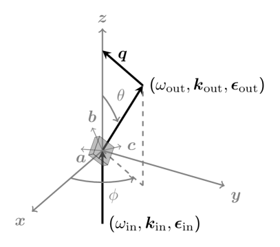
Figure 1: Scattering geometry for photon-in/photon-out spectroscopy. For $\phi=0$, $\boldsymbol{\epsilon}_{\rm in}$ points along $\boldsymbol{x}$. The gray box represents the sample as a single crystal, where the cell vectors ($\boldsymbol{a}$, $\boldsymbol{b}$, $\boldsymbol{c}$) are not oriented with respect to the surface in order to emphasise the polarization effects.

X-ray emission is a secondary process that occurs after creation of a vacancy in an inner-shell of the element of interest. In most applications this vacancy is created after photoexcitation and x-ray emission becomes a photon-in/photon-out process and therefore an x-ray scattering phenomenon. Alternatives to photoexcitation exist (e.g. ion or electron bombardement, radioactive isotopes) but the theoretical treatment in these cases only requires minor adjustments with respect to the following considerations. In the general description of a scattering process (cf. figure 1 for the scattering geometry), a photon of energy $\hbar\omega_{\rm in}$, wave vector $\boldsymbol{k}_{\rm in}$ and unit polarization vector $\boldsymbol{\epsilon}_{\rm in}$ is scattered by the sample with ground state eigenfunction $\left|g\right\rangle$. A photon is emitted into a solid angle $d\Omega$ described by a polar angle $\theta$ and azimuthal angle $\phi$. The scattered photon has energy $\hbar\omega_{\rm out}$, wave vector $\boldsymbol{k}_{\rm out}$ and polarization $\boldsymbol{\epsilon}_{\rm out}$. The energy $\hbar\omega=\hbar(\omega_{\rm in}-\omega_{\rm out})$ and momentum $\hbar\boldsymbol{q}=\hbar(\boldsymbol{k}_{\rm in}-\boldsymbol{k}_{\rm out})$ are transferred to the sample that consequently makes a transition from the ground state $\left|g\right\rangle$ with energy $E_{g}$ to the final state $\left|f\right\rangle$ with energy $E_{f}$. The derivation of the double differential scattering cross-section (DDSCS), $d^{2}\sigma/(d\Omega d\hbar\omega_{\rm out})$, by means of second-order perturbation treatment can be found in many textbooks (e.g. Schülke Schülke (2007) and Sakurai Sakurai (1967)). The x-ray electromagnetic field is represented by its vector potential $\boldsymbol{A}$. By neglecting the interaction of the magnetic field with the electron spin, the interaction Hamiltonian is written (in SI units) as Ament et al. (2011)

$$H_{\rm int}=\frac{e^{2}}{2m}\sum_{j}\boldsymbol{A}(\boldsymbol{r}_{j})^{2}+\frac{e}{m}\sum_{j}\boldsymbol{p}_{j}\cdot\boldsymbol{A}(\boldsymbol{r}_{j})$$ (1)

where $\boldsymbol{p}_{j}$ is the momentum of the $j$-th target electron. The transition probability is given by the golden rule $\left\langle s_{2}\right|T\left|s_{1}\right\rangle$ where $T$ is a transition operator connecting two eigenstates. The term containing $\boldsymbol{A}^{2}$ does not involve the creation of a photon-less intermediate state and can therefore be described as a one-step scattering process (first order perturbation theory term). It gives rise to non-resonant scattering and can, apart from a few exceptions, not be used for an element-selective spectroscopy. The non-resonant term accounts for elastic Thomson scattering and inelastic Raman and Compton scattering. Inelastic scattering may give an element-selective signature if the energy transfer corresponds to an absorption edge Schülke (2007) (the case of XRS).
The term containing $\boldsymbol{p}\cdot\boldsymbol{A}$ contributes to the second order perturbation term and causes annihilation of the incoming photon and thus the creation of an intermediate state that lives for a time $\tau$ and decays upon emission (creation) of a photon. The technique is element-selective if the intermediate state can be represented by an electron configuration that contains a hole in a core level of the element of interest. As in example, for Mn this would be the levels 1$s$, 2$s$, …, 3$p$ (cf. figure 2).

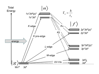
Figure 2: Total energy diagram of a system containing Mn in formal oxidation state III. The energy levels for the ground ($\left|g\right\rangle$), intermediate ($\left|n\right\rangle$) and final ($\left|f\right\rangle$) states are approximated using atomic configurations and a single-particle picture of the electronic transitions. Closed shells are omitted for clarity. Black lines indicate that each configuration corresponds to a collection of several many-body states. Rectangles symbolise a band state, where the notation (p) represents mixed states between the atomic 4$p$ level and the bands of the solid. The notation L corresponds to a hole created on a ligand orbital. Solid-line arrows indicate the absorption edge that allows the corresponding excited state to be reached directly, i.e. in one step. Dashed-line arrows indicate the emission line that allows excited states of lower energies to be reached in a second step, i.e. after a core hole has been primarily created. Inspired from Figure 2.3 in Ref. Glatzel and Juhin, 2013.

We refer to the resonant term as the Kramers-Heisenberg cross section. This term governs x-ray absorption (when considered as coherent elastic forward scattering) and x-ray emission including all resonant scattering processes. The interaction terms can be treated separately, assuming implicitly that the experimental conditions are chosen such that one term dominates. Other terms and interference with them are not taken into account. Removing unimportant factors, the essential part of the RIXS spectrum can be described in the following form Schülke (2007)

$$\sigma(\omega_{\rm in},\omega_{\rm out}) = r_{e}^{2}\frac{\omega_{\rm out}}{\omega_{\rm in}}\sum_{f}\left|\sum_{n}\frac{\left\langle f\right|T_{\rm out}^{*}\left|n\right\rangle\left\langle n\right|T_{\rm in}\left|g\right\rangle}{E_{g}-E_{n}+\hbar\omega_{\rm in}-i\Gamma_{n}/2}\right|^{2}$$ (2)

$$\times \delta(E_{g}-E_{f}+\hbar\omega_{\rm in}-\hbar\omega_{\rm out})$$

where $r_{e}$ is the classical electron radius and $T$ the transition operators ($T=\sum_{j}(\boldsymbol{\epsilon}\cdot\boldsymbol{p}_{j})e^{i\boldsymbol{k}\cdot\boldsymbol{r}_{j}}$). $\Gamma_{n}$ denotes the spectral broadening due to the core hole lifetime of the intermediate state $\left|n\right\rangle$ as a result of the Auger and radiative decays of the core hole. The lifetime is often assumed constant for a given subshell core hole. In order to account for the finite lifetime of the final states, the energy-conservation $\delta$-function can be broadened into a Lorentian of full width at half maximum $\Gamma_{f}$: $\frac{\Gamma_{f}/2\pi}{(E_{g}-E_{f}+\hbar\omega_{\rm in}-\hbar\omega_{\rm out})^{2}+\Gamma_{f}^{2}/4}$. A final approximation that is employed for practical calculation of the Kramers-Heisenberg cross section is the expansion to the second order of the transition operators. This leads to $T\approx\boldsymbol{\epsilon}\cdot\boldsymbol{r}+\frac{i}{2}(\boldsymbol{\epsilon}\cdot\boldsymbol{r})(\boldsymbol{k}\cdot\boldsymbol{r})$ and corresponds to a description of the cross section in terms of dipole (E1) and quadrupole (E2) transitions only.

II.1 Kramers-Heisenberg equation for XES

The Kramers-Heisenberg equation (Eq. 2) is the basis for x-ray absorption and emission spectroscopy. We note that this view is at odds with some publications where the Kramers-Heisenberg equation is only applied to excitations just above ($\approx$ 0-20 eV) the Fermi level. Such excitations are referred to as resonances. However, also x-ray emission after photoionization has to be treated using the formalism of Eq. 2 and there is no fundamental difference between excitations close to or well above the Fermi level. Interference effects may be more likely to be important just above an absorption edge but this does not suffice for a clear distinction.

Figure 3: Simplified total energy diagram for XES. A continuum of intermediate and final states is reached whose energies depend on the photoelectron kinetic energy $\varepsilon$. Several of these pairs of states may exist (with different $n^{\prime}$, $f^{\prime}$ and $\varepsilon$) that need to summed up for a full treatment of the x-ray emission process after photo excitation.

The cross section changes dramatically within the first tens of eV above an absorption edge and approaches a $\frac{1}{E^{3}}$ dependence. In this range, the photoelectron (described by its energy $\varepsilon$) does not interact with the remaining ion; the intermediate and final states with their energies are written as Ljungberg et al. (2010) $\left\langle n\right|=\left\langle n^{\prime}\right|\left\langle\varepsilon\right|$, $E_{n}=E_{n^{\prime}}+\varepsilon$ and $\left\langle f\right|=\left\langle f^{\prime}\right|\left\langle\varepsilon\right|$, $E_{f}=E_{f^{\prime}}+\varepsilon$ (cf. figure 3). The photoelectron does not change its energy upon the radiative decay of the ion. One thus obtains, for each ionic intermediate and final state, $n^{\prime}$ and $f^{\prime}$, an infinite number of states characterised by the kinetic energy of the photoelectron. Eq. 2 then becomes

$$\sigma(\omega_{\rm in},\omega_{\rm out})\propto$$

$$\sum_{f^{\prime}}\sum_{n^{\prime}}\int_{\varepsilon}\left|\frac{\left\langle f^{\prime}\right|\left\langle\varepsilon\right|T_{\rm out}^{*}\left|\varepsilon\right\rangle\left|n^{\prime}\right\rangle\left\langle n^{\prime}\right|\left\langle\varepsilon\right|T_{\rm in}\left|g\right\rangle}{E_{g}-(E_{n^{\prime}}+\varepsilon)+\hbar\omega_{\rm in}-i\Gamma_{n}/2}\right|^{2}$$

$$\times\frac{\Gamma_{f}/2\pi}{(E_{g}-(E_{f^{\prime}}+\varepsilon)+\hbar\omega_{\rm in}-\hbar\omega_{\rm out})^{2}+\Gamma_{f}^{2}/4}$$ (3)

We assume constant absorption and emission matrix elements for each $n^{\prime}$, $f^{\prime}$, i.e. independent of the photoelectron kinetic energy $\varepsilon$ (which is justified over a small energy range), and we obtain

$$\sigma(\omega_{\rm in},\omega_{\rm out})\propto$$

$$\sum_{f^{\prime}}\sum_{n^{\prime}}\left|\left\langle f^{\prime}\right|\left\langle\varepsilon\right|T_{\rm out}^{*}\left|\varepsilon\right\rangle\left|n^{\prime}\right\rangle\left\langle n^{\prime}\right|\left\langle\varepsilon\right|T_{\rm in}\left|g\right\rangle\right|^{2}$$

$$\times\int_{\varepsilon}\frac{1}{(E_{g}-(E_{n^{\prime}}+\varepsilon)+\hbar\omega_{\rm in})^{2}+\Gamma_{n}^{2}/4}$$

$$\times\frac{\Gamma_{f}/2\pi}{(E_{g}-(E_{f^{\prime}}+\varepsilon)+\hbar\omega_{\rm in}-\hbar\omega_{\rm out})^{2}+\Gamma_{f}^{2}/4}$$ (4)

The integral over $\varepsilon$ is a convolution of two Lorentzian functions which gives a Lorentzian as a function of $\omega_{\rm out}$ with width $\Gamma_{n}+\Gamma_{f}$ which is the known result for non-resonant fluorescence spectroscopy. A broad energy bandwidth for the incident beam will result in a larger range of photoelectron kinetic energy but not influence the width of the convoluted Lorentzian. Hence, the spectral broadening is independent of the incident energy bandwidth. This opens the door to experiments using non-monochromatic radiation with a bandwidth of $\Delta E<100$ eV (pink beam) at synchrotron radiation sources or free electron lasers Kern et al. (2013).
The spectral shape does not depend on $\varepsilon$ as long as the same set of intermediate states $n^{\prime}$ is reached. This may change if the incident energy suffices to create more than one core hole (cf. Ref. Hoszowska and Dousse, 2013 and references therein). One example is the KL-edge where one incident photon creates a hole in the K- and L-shell. This may significantly alter the x-ray emission spectral shape. It is therefore important to choose the incident energy below the edge of multi-electron excitations, if possible.

III Approaches to the calculations

In this section we will present a short overview of the methods currently employed to calculate the experimental spectra. The theoretical simulation is an important tool for the experimentalist who needs to analyse the collected spectra and to plan new experiments. We can roughly separate the various approaches to the calculations of inner-shell spectra into two main philosophies, that we can refer to as: many-body atomic picture and single-particle extended picture. They are based, respectively, on ligand field multiplet theory (LFMT) and density functional theory (DFT).
In LFMT one first considers a single ion and writes its wavefunction as a single or linear combination of Slater determinants of atomic one-electron wavefunctions. The chemical environment is then considered by empirically introducing the crystal field splittings and the orbital mixing. A detailed description of LFMT can be found in textbooks Bransden and Joachain (1983); Figgis and Hitchman (2000); De Groot and Kotani (2008) or topical reviews Griffith and Orgel (1957); de Groot (2001, 2005), while a tutorial-oriented description of the calculations was given by van der Laan van Der Laan (2006). The codes currently in use are those developed by Cowan Cowan (1968, 1981) in the sixties and extended by Thole in the eighties (cf. Ref. van der Laan, 1997 for a technical overview). Recently, a user friendly interface, ctm4xas Stavitski and de Groot (2010), has permitted a larger community accessing such calculations. The advantage of this approach is that the core hole is explicitely taken into account and multi-electron effects are calculated naturally by applying multiplet theory. The obvious problem with this approach is that the chemical environment is only considered empirically.
In the DFT-based approach, a simplified version of the Schrödinger equation is solved either for a cluster of atoms centered around the absorbing one (real space method) or using periodic boundary conditions (reciprocal space method). This means that the electronic structure is calculated ab initio, without the need of empirical parameters, and the results depend on the level of approximation employed. Among the large number of presently used codes, the most common techniques are: multiple scattering theory (e.g. feff9 Rehr et al. (2010, 2009), fdmnes Joly (2001); Bunău and Joly (2009) and mxan Benfatto and Della Longa (2001)), full potential linearised augmented plane wave, FLAPW (e.g. Wien2k Schwarz and Blaha (2003); Pardini et al. (2012)), projector augmented-wave method, PAW (e.g. quantum-espresso Giannozzi et al. (2009); Gougoussis et al. (2009); Bunǎu and Calandra (2013), gpaw Enkovaara et al. (2010); Ljungberg et al. (2011), bigdft Genovese et al. (2008)) and time-dependent DFT (e.g. orca Neese (2012); Debeer George and Neese (2010)). The advantage in the DFT approach is that the theoretical framework is well established and numerous groups work on evaluating and improving the level of theory, i.e. the exchange-correlation functionals or the basis sets. However, DFT is a theory to calculate the ground state electronic structure which is a priori incompatible with inner-shell spectroscopy. Furthermore, in its basic implementation, DFT calculates one-electron transitions which are insufficient when the inner-shell vacancy gives a pronounced perturbation of the electronic structure, resulting in important many-body effects. These shortcomings have been addressed within DFT and considerable progress has been made Onida and Rubio (2002).
The decision on which approach is most suitable for the problem at hand can be based on the degree of localization of the orbitals that are assumed to be involved in the transitions. The K absorption main edge in 3$d$ transition metals is often modeled using DFT. The pre-edge requires a mixture of atomic and extended view and therefore only in a few favorable cases a good understanding of the pre-edge features has been achieved. The L-edges of rare earths and 5$d$ transition metals require an extended approach. However, 2$p$ to 4$f$ transitions that form the L pre-edge in rare earths are highly localised and an atomic approach is very successful. The K$\beta$ main line emission in 3$d$ transition metals involve atomic orbitals. Multiplet theory can therefore reproduce the spectral shape to high accuracy. In contrast, the valence-to-core lines involve molecular orbitals that are mainly localised on the ligands and a one-electron DFT approach is therefore very succesful in reproducing the spectra.
It is often illuminating to apply a very simplified approach to simulate an experimental result, as it permits assessing what interactions and effects are relevant. As an example, if one neglects interference effects, the core hole potential and multi-electron transitions, it is possible to drastically simplify the Kramers-Heisenberg formula (Eq. 2) for the case of valence-to-core RIXS and obtain an expression in terms of the angular momentum projected density of states Jiménez-Mier et al. (1999)

$$\sigma(\omega_{\rm in},\omega_{\rm out})\propto\int_{\varepsilon}\frac{\rho(\varepsilon)\rho^{\prime}(\varepsilon+\omega_{\rm in}-\omega_{\rm out})}{(\varepsilon-\omega_{\rm out})^{2}+\Gamma_{n}^{2}/4}d\varepsilon$$ (5)

where $\rho$ and $\rho^{\prime}$ are, respectively, the occupied and unoccupied density of states, $\Gamma_{n}$ the lifetime broadening of the intermediate state. This approach has been demonstrated valid in describing the VTC-RIXS spectra of 5$d$ transition metal systems Smolentsev et al. (2011); Garino et al. (2012). A similar approach but partly considering the core hole potential and the radial matrix element was recently implemented in the feff9 code Kas et al. (2011).
The combination of an extended picture with full multiplet calculations is the holy grail in theoretical inner-shell spectroscopy. The progress in recent years has been impressive to the great benefit of the experimentalists who are gradually getting a better handle on analyzing their data Mirone et al. (2000); Uldry et al. (2012); Mirone (2012). A promising method is to make use of maximally localised Wannier functions Marzari et al. (2012) as directly obtained from DFT calculations. If one extracts the Wannier orbitals in the bands near the Fermi level, is then possible to calculate the spectra via LFMT Haverkort et al. (2012). However, this method is still an approximate solution of the problem. A more rigorous treatement was proposed in the framework of the multi-channel multiple scattering (MCMS) theory Natoli et al. (1990) (recently revised in Ref. Natoli et al., 2012). The MCMS method has been successfully applied in simulating the L_2,3 XAS spectra of Ca Krüger and Natoli (2004) and Ti Krüger (2010) and could be easily extended to XES and RIXS.

IV Experimental set-up

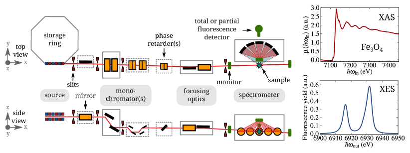
Figure 4: Schematic view (top/side) of a generic hard x-ray RIXS-dedicated beamline: optics and experimental stations (cf. description in the text). The represented objects are not in scale and do not represent a given technical design. Right panels show an example of XAS (scanning the incoming energy, $\hbar\omega_{\rm in}$, top) and XES (scanning the outgoing energy, $\hbar\omega_{\rm out}$, bottom) spectra of Fe₃O₄ powder obtained at the Fe K-edge.

Before presenting a selection of applications of the technique, we describe how a combined XAS/XES experiment is performed on a generic synchrotron radiation beamline. This is schematically illustrated in figure 4. The synchrotron radiation is produced in the storage ring via an undulator, bending magnet or wiggler (source). A first collimating mirror, run in total reflection geometry, is usually used to reduce the heat load, collimate the beam and remove the higher harmonics. The beam is then monochromatised by a double single crystal monochromator (cryogenically cooled); typically two pairs of crystals are employed: Si(111) or Si(311), giving an intrinsic (without taking into account the beam divergence) resolving power, $\frac{E}{\Delta E}$, of 7092 and 34483 Matsushita and Hashizume (1983), respectively. The monochromatic beam is then focused to the sample via a focusing system, typically, two bent mirrors in Kirkpatrick-Baez geometry Kirkpatrick and Baez (1948), that is, working in glancing incidence (around 3 mrad), one focusing horizontally and the second one, perpendicular to the previous, focusing vertically. A given number of slits (vertical and horizontal) is also inserted in the beam path to clean for aberrations and reduce the divergence. In addition, the beamline optics can be complemented with a second monochromator or phase retarders. The second monochromator, typically a channel cut in four crystals configuration DuMond (1937), is used to improve the energy resolution. The phase retarders Giles et al. (1995), typically thin diamond crystals put in diffraction conditions, permit tuning the polarization of the x-ray beam. In fact, apart for helical undulators, the x-ray beam is linearly polarised in the orbital plane and the phase retarders are required for generating circularly polarised light (left and right) or linearly polarised in the vertical plane.
In the experimental station, the equipment is built around the sample stage (figure 4). The main elements consist in x-ray detectors for monitoring the incoming and transmitted beam and measuring the fluorescence emitted by the excited sample. For hard x-rays, the sample environment does not require a vacuum chamber and it is quite versatile: a goniometer permits aligning the sample in three dimensions plus hosting additional equipments (e.g. cryostat, furnace, magnet or chemical reactor). For bulk samples, the XAS (absorption coefficient, $\mu(\hbar\omega_{\rm in})$) is measured directly via the intensity of the incoming ($I_{\rm in}$) and transmitted beam ($I_{\rm out}$), according to the Beer-Lambert law: $I_{\rm out}=I_{\rm in}e^{-\mu(\hbar\omega_{\rm in})x}$, where $x$ is the sample’s thickness. For dilute species, $\mu$ cannot be measured directly and a secondary process (yield) has to be employed, assuming that the absorption cross section is proportional to the number of core holes created. The secondary processes can be either the collection of the electron yield Erbil et al. (1988) or the fluorescence yield Jaklevic (1977). We will not treat the electron yield here, but focus on the fluorescence yield (FY) because this gives access to a photon-in/photon-out spectroscopy, as XES and RIXS. Usually, the FY-XAS is collected either without energy resolution (total FY) or with an energy dispersive solid state detector (SSD) as an array of high purity germanium elements or silicon drift diodes. For linearly polarised synchrotron radiation (with $\boldsymbol{\epsilon}_{\rm in}$ along $\boldsymbol{x}$, cf. figure 1, as in standard experiments) the Thomson (elastic), Compton and Raman (inelastic) scattering have an angular dependence of $sin^{2}(\phi)+cos^{2}(\theta)cos^{2}(\phi)$ (cf. figure 1) while the fluorescence emitted by the sample is isotropic (in a standard geometry and not considering polarization effects, cf. Ref. Bianchini and Glatzel, 2012 for the full expression), thus the fluorescence detectors are usually put at 90 degrees on the polarization plane to minimise the background due to scattering (cf. figure 4). SSD detectors permit a typical energy resolution of 150-300 eV ($\frac{E}{\Delta E}$ $\approx$ 50). This low energy resolution combined with a low saturation threshold is a drawback for measuring dilute species in strong absorbing matrices as DMS/CMS. In fact, the weak signal of interest is very often sitting on the strong background coming from the low-energy tail of the Thompson and Compton scattering or overlapping with the fluorescence lines of the other elements contained in the matrix. For thin films deposited on a substrate, a workaround for collecting a clean fluorescence signal is to work in a combined grazing incidence and grazing exit geometry Maurizio et al. (2009) but this has the drawback of fixing the experimental geometry and it is not suitable for single crystals where it is important also to work with the polarization axis laying out of the sample surface. An increased energy resolution ($\frac{E}{\Delta E}$ $\approx$ 1000) can be obtained with charged coupled devices Fourment et al. (2009) or microcalorimetric arrays Uhlig et al. (2013) used in energy resolving mode. However, the complexity of these detectors (especially in the events reconstruction algorithms) and the very quick saturation for calorimeters, limits their application on standard spectroscopy beamlines.
In order to overcome these limitations and to collect XES, RIXS and HERFD-XAS, a wavelength dispersive spectrometer has to be employed ($\frac{E}{\Delta E}$ $>$ 5000). For hard x-rays, this means that Bragg’s diffraction over an analyser crystal is employed to monochromatise the emitted fluorescence from the sample (Rowland’s circle geometry). Among all the possible diffraction geometries Jalal and Golamreza (2011), two main configurations are currently in use at synchrotron facilities: the point-to-point Johann Johann (1931) and the dispersive Von Hamos v. Hámos (1933). For both, the basic principle is that the source (sample), the diffractor (analyser crystal) and the image (detector) are on the Rowland circle. The first class uses spherically bent crystals Verbeni et al. (2005) in combination with one-dimension detector; the energy selection is performed by scanning the crystal Bragg’s angle and the detector over the Rowland circle. In the second class, a cylindrically bent crystal is combined with a position-sensitive detector; the energy dispersion is obtained without moving the crystal and by collecting the different areas of the detector. Without going into the details of the advantages and disadvantages of each configuration, good performances are obtained with an increased number of spherically bent crystals (to overcome the small solid angle collected, $\approx$ 0.03 sr per crystal) working at Bragg’ angles close to 90 deg. As few examples of currently available instruments, there are those dedicated to XRS Verbeni et al. (2009); Sokaras et al. (2012), medium-resolution RIXS Glatzel et al. (2009); Kleymenov et al. (2011); Llorens et al. (2012); Sokaras et al. (2013) and single-shot XES Szlachetko et al. (2012); Alonso-Mori et al. (2012).

V The RIXS plane and sharpening effects

An experimental 1$s$2$p$ RIXS intensity plane is shown in figure 5 in the incident ($\hbar\omega_{\rm in}$) versus transfer ($\hbar\omega_{\rm in}-\hbar\omega_{\rm out}$) energy axis. The transitions to continuum (main absorption edge) appear as dispersive features along the diagonal, while the transitions to localised states (pre-edge features) appear as resonances at well defined positions in the plane. The two groups of diagonal features visible in figure 5 are vertically split by the 2$p$ spin-orbit interaction in the final state, corresponding to the K$\alpha_{1}$ and K$\alpha_{2}$ emission lines. A diagonal cut (constant emitted energy) will then give the HERFD-XAS spectrum, while an integration over the vertical direction results in a standard XANES spectrum. Considering only the pre-edge region, a vertical cut (constant incident energy) gives a spectrum sentitive to the spin-orbit interaction in the final state and the exchange interaction between the intermediate and final states. This is similar to L_2,3 edges XAS. A cut in the horizontal direction (constant final state energy) is affected by the spin-orbit and exchange interaction in the intermediate state only. On the other hand, analyzing RIXS data as line scans can lead to false interpretation of the spectral features. For example, the two pre-edge peaks in figure 5 have an incoming energy separation of 1.8 eV that would be underestimated (1.4 eV) if a peak-fitting procedure is employed on the HERFD-XAS scan. This is due to the fact the the first resonance does not lie on the diagonal of the RIXS plane (cf. figure 5).

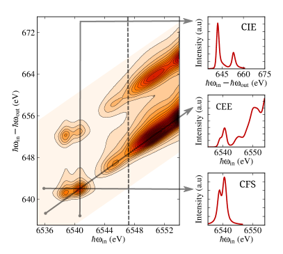
Figure 5: 1$s$2$p$ RIXS intensity plane for a Ga_0.97Mn_0.03N thin film (cf. Ref. Stefanowicz et al., 2010 for the sample’s growth and characterization). The insets show line cuts in three main directions: at constant incident energy (CIE = energy loss), constant emitted energy (CEE = HERFD-XAS) and constant final state energy (CFS). The vertical dashed line indicates the absorption edge position.

One appreciated feature of RIXS/HERFD-XAS is a dramatic improvement in resolving the spectral features (sharpening effect). The effect is striking at the L_2,3 edges of 5$d$ elements when compared to standard XANES while at K pre-edge of 3$d$ elements permits catching fine details due to the strong reduction of the background signal. For example, HERFD-XAS has permitted precisely following catalytic reactions Hartfelder et al. (2013) or to reveal angular-dependent core hole effects Juhin et al. (2010). The origin of the sharpening effect was attributed to interference causing the elimination of the core hole broadening Hämäläinen et al. (1991). Actually, the interference does not play a role here and the lifetime broadenings are still present, as shown by the elongated features in the horizontal and vertical direction of the RIXS plane (cf. figure 5). Without going into the details of the difference between HERFD-XAS and standard XAS spectra, as previously discussed by Carra et al. Carra et al. (1995), it was demonstrated that the improved resolution of the experimental spectra can be reproduced by an apparent broadening de Groot et al. (2002)

$$\Gamma_{\rm exp}\approx\frac{1}{\sqrt{(1/\Gamma_{n})^{2}+(1/\Gamma_{f})^{2}}}$$ (6)

where the intermediate ($\Gamma_{n}$) and final ($\Gamma_{f}$) core hole lifetime broadenings are taken into account.

VI Valence states sensitivity of K fluorescence lines

The macroscopic properties of semiconductors (e.g. transport, magnetism) are driven by impurities (defects) located at valence states. Accessing the information of such states via a bulk probe, permits then having a detailed description of the material under study. XES can probe valence electrons either indirectly or directly, by selecting the yield for different transitions. If one collects core-to-core (ctc) transitions, the valence electrons are probed indirectly, while directly for valence-to-core (vtc). The selectivity to the electronic structure of the valence shell in CTC-XES originates from screening effects (the core levels energy is affected by the modified nuclear potential) and multiplet structure (the spin and orbital angular momentum of the core hole strongly couple to the valence electrons). The screening dominates for light elements as, for example, the K$\alpha$ XES of S Alonso Mori et al. (2009), while the multiplet structure dominates in the case of the K fluorescence lines of 3$d$ TMs.

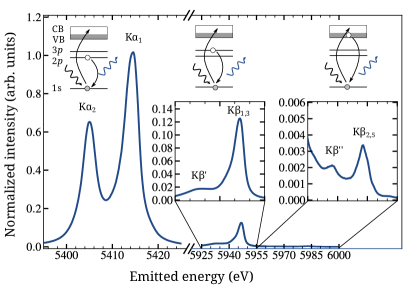
Figure 6: XES spectrum of Cr₂O₃ showing the Cr K fluorescence lines (blue): CTC-K$\alpha$, CTC-K$\beta$ and VTC-K$\beta$. In the plots the intensity is normalised to the K$\alpha_{1}$ maximum; the insets show an expanded view for CTC-K$\beta$ and VTC-K$\beta$. The top schemes show the origin of the transitions after photoionization in a simplified one-electron picture. Black lines indicate core states (1$s$, 2$p$, 3$p$), while the rectagles symbolise the valence and conduction bands (VB and CB).

A XES spectrum is given in figure 6 for Cr in Cr₂O₃. The most intense lines are the K$\alpha_{1}$ (K-L₃, 2$p_{3/2}$ $\to$ 1$s$) and K$\alpha_{2}$ (K-L₂, 2$p_{1/2}$ $\to$ 1$s$), where the 2$p$ level is splitted by the strong spin-orbit interaction. With $\approx$ 10-times smaller intensity are visible the CTC-K$\beta$ lines (K-M_2,3, 3$p$ $\to$ 1$s$), called Tsutsumi (1959) K$\beta_{1,3}$ (main peak) and K$\beta^{\prime}$ (broad shoulder at lower emitted energy). Finally, the VTC-K$\beta$ lines appear on the tail of the main lines with roughly 200-times smaller intensity, those are called K$\beta_{2,5}$ and K$\beta^{\prime\prime}$. The origin and information content of CTC-K$\beta$ lines is given later in § VII, while here we focus first on VTC-K$\beta$ lines.
The VTC-K$\beta$ arise from transitions from occupied orbitals a few eV below the Fermi level (the valence band), that is, from orbital mixed metal-ligand states of metal $p$-character to 1$s$. For this reason, VTC-K$\beta$ is strongly sensitive to ligand species and has been employed in chemistry to distinguish between ligands of light elements Bergmann et al. (1999); Safonov et al. (2006); Eeckhout et al. (2009); Lancaster et al. (2011) (e.g. C, N, O, S). In addition, by making use of the XES polarization dependence Glatzel and Bergmann (2005) is possible to study the orientation of the lingands. For example, Bergmann et al. Bergmann et al. (2002) studied a Mn nitrido coordination complex in $C_{4v}$ symmetry with five CN and one N ligand at a very short distance (1.5 Å). The signal arising from the nitrido molecular orbitals was almost completely suppressed by orienting the Mn-nitrido bond in the direction of $\boldsymbol{k}_{\rm out}$, i.e. towards the crystal analyser. Another advantage of VTC-K$\beta$ is the possibility to easily calculate the transitions with a molecular-orbital approach: from early atomic Best (1966) to recent DFT methods Pollock and DeBeer (2011); Gallo et al. (2011); Vila et al. (2011). These works demonstate that the K$\beta^{\prime\prime}$ and K$\beta_{2,5}$ are mainly sensitive, respectively, to the ligand $s$ and $p$ states. The K$\beta_{2,5}$ has also a strong dependece on the metal’s local symmetry Smolentsev et al. (2009); Gallo et al. (2013) (e.g. T_D vs O_h). For a more rigorous treatement, the interested reader can refer to a recent topical review Gallo and Glatzel (2014).

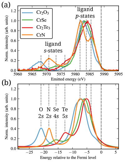
Figure 7: VTC-K$\beta$ spectra for a selected set of Cr-based compounds. Top panel (a): experimental data - after removal of the CTC-K$\beta$ background and normalization to the K$\beta_{2,5}$ peak maximum - from commercially available powders. Bottom panel (b): ab initio simulations with the fdmnes code (cf. details in the text). The ligands’ states sensitivity of K$\beta^{\prime\prime}$ and K$\beta_{2,5}$ is outlined. Vertical dashed lines are a guide for the eye to compare the main spectral features between the simulation and the experiment.

In DMS, one application of VTC-K$\beta$ is in the study of the interaction of shallow dopants with the metal site. For example, in Zn_1-xCr_xTe co-doped with N Kuroda et al. (2007), where N is an acceptor (brings holes in the valence band), by measuring the Cr VTC-K$\beta$ it is possible to detect when N interacts with Cr via the clear signature of N 2$s$ levels in the Cr K$\beta^{\prime\prime}$. This is illustrated in figure 7 where we show a selection of VTC-K$\beta$ spectra for commercially available Cr-based powder compounds compared with the ab initio simulations (fdmnes code Bunău and Joly (2009)). Standard crystal structures (retrieved from the “Inorganic Crystal Structure Database”, FIZ Karlsruhe) are used as input in the calculations, conducted in real space with a muffin-tin approximation and the Hedin-Lundqvist exchange-correlation potential. To compare with the experiment, the calculated Fermi levels are arbitrarily shifted and the spectra are convoluted with a constant Lorentian broadening of 2.68 eV. The origin of the features is then attributed by selecting the projected density of states on the ligands that overlaps with the metal $p$ one (not shown). This confirms previous works, that is, the K$\beta^{\prime\prime}$ mainly comes from the ligand $s$ states, while the K$\beta_{2,5}$ is from the ligand $p$ states. As shown in figure 7, the energy position of the K$\beta^{\prime\prime}$ is very sensitive to the type of ligand and permits identifying if a compound has an additional phase. For example, the experimental Cr₂Te₃ spectrum shows a second K$\beta^{\prime\prime}$ at 5967 eV, corresponding to oxygen, that is not reproduced in the calculation. The origin of this extra feature is then easily understood by the fact that Cr₂Te₃ is an air-sensitive compound and, due to the measurements carried in air, it was contaminated by oxygen. The analysis of the K$\beta_{2,5}$ is more demanding, because its spectral features are also affected by the local symmetry. This effect is also shown in figure 7, where the simulated and experimental K$\beta_{2,5}$ do not fully align. One reason resides in the fact that the simulation takes into account only one crystallographic structure, while the commercial powders may contain more than one crystal phase of the same compound.

VII K$\beta$ spin sensitivity via intra-atomic exchange interaction

The analysis of the CTC-K$\beta$ is of particular interest for magnetic semiconductors because it permits probing (indirectly) the local magnetic moment brought by the 3$d$ TMs impurities without the need of demanding sample environment as low temperature and high magnetic field. In fact, CTC-K$\beta$ is sensitive to the net local 3$d$ spin moment, independently of its direction. This gives the possibility to study a magnetic material even in the paramagnetic state, that is, when the local moments are fluctuating and pointing in random directions. As shown in figure 8 for three Mn-Oxide powder samples (MnO, Mn₂O₃, MnO₂), the K$\beta$ main lines evolve with the decreasing nominal spin state ($S$, $S_{\rm MnO}$ = 2.5 $\to$ $S_{\rm MnO_{2}}$ = 2): the K$\beta_{1,3}$ shifts toward lower energy and the K$\beta^{\prime}$ reduces in intensity; this means that the center of mass energy (the sum of the energies of all final states weighed by their intensities) does not change between the configurations but the K$\beta_{1,3}$-K$\beta^{\prime}$ splitting decreases with decreasing spin state. This behaviour is understood in a total energy diagram (inset of figure 8). The intra-atomic exchange energy between the 3$p$ hole and the 3$d$ levels (sum of the Slater exchange integrals, $J$) lowers the total energy. As a consequence, the configurations with parallel spins are lower in energy than the configurations with paired spins.

Figure 8: Evolution of the CTC-K$\beta$ spectra for MnO, Mn₂O₃ and MnO₂. The inset shows this evolution in terms of the total energy; for simplicity, only one spin configuration is taken into account and paired electrons are omitted.

The K$\beta$ transition involves core levels and multiplet ligand-field theory is therefore the appropriate framework to discuss the spectral features de Groot et al. (1994b); Peng et al. (1994a); Wang et al. (1997). In order to better understand the spin-polarised origin of the K$\beta$ emission for a 3$d$ TM, we take as example the 3$d^{5}$ configuration, an atomic picture and a two-step process Glatzel et al. (2001) (as shown in figure 9a). A 3$d^{5}$ high spin configuration is a favorable case because of the absence of an orbital angular momentum in the ground state. Hund’s rule dictates that all spins are aligned, giving the ${}^{\rm 6}\mathrm{S}$ ground state spin-orbit term. Photoionization then excites the system to the 1$s$3$d^{5}$+$\varepsilon p$ (${}^{\rm 5,7}\mathrm{S}$) intermediate states. The ${}^{\rm 7}\mathrm{S}$ term can only decay into the ${}^{\rm 7}\mathrm{P}$, while the ${}^{\rm 5}\mathrm{S}$ one decays into all interacting ${}^{\rm 5}\mathrm{P}$ states (where symmetry mixing is important). In consequence, the K$\beta^{\prime}$ originates almost 100% from spin-up transitions and the K$\beta_{1,3}$ primarly from spin-down. This result is exemplified in figure 9b via a one-electron picture of the final state. In Ref. Wang et al., 1997, the strong spin selectivity was demonstrated valid also when the atom is inserted in a crystal field. In fact, neglecting orbital mixing, the K$\beta$ lines do not depend on the fine structure in the valence shell (e.g. crystal field splitting) as long a the spin state does not change. On the other hand, a strong crystal field splitting may result in a low spin configuration which will change the K$\beta$ line shape Badro et al. (2003). These considerations are valid for O_h symmetry. For T_D symmetry, the strong spin polarization is still present because the crystal field splitting, 10Dq, is simply inverted between the two symmetries. In addition, the absence of inversion symmetry (in contrast to O_h) results in strong $pd$ mixing. Including orbital mixing in the theoretical description, may find that the 3$p$3$d$ exchange interaction changes owing to the mixing and thus the shape of K$\beta$ lines varies. In conclusion, the spin selectivity is conserved and it is employed to record spin-selective XAS (cf. § VII.1), while the spectral features change and the methods to take them into account are discussed in the following.

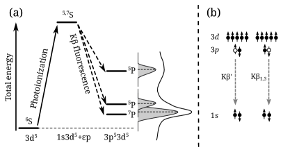
Figure 9: K$\beta$ emission process after photoionization illustrated for a 3$d^{5}$ case. Left panel (a): atomic multiplet theory. Right panel (b): simplified one-electron picture (not in energy scale) where paired electrons and the spin flipping in K$\beta_{1,3}$ are omitted for clarity. A detailed description is given in the text.

To perform quantitative analysis of the CTC-K$\beta$, the first method is to approximate the energy separation and the intensity ratio between K$\beta_{1,3}$ and K$\beta^{\prime}$ by $\Delta E=J(2S+1)$ and $I^{\prime}/I_{1,3}=S/(S+1)$ Tsutsumi et al. (1976). This approximation is found to reproduce fairly well the experimental results if a peak fitting procedure is employed Gamblin and Urch (2001); Torres Deluigi et al. (2006); Bergmann et al. (1998). On the other hand, a peak fitting procedure is prone to errors in the extraction of the peaks positions and arbitrary in the choice of the number and form of the fitted functions. To overcome the problem of linking the data analysis to a theoretical approximation, fully experimental data reduction methods were put in place. The first attempt was to use the first moment energy of the K$\beta_{1,3}$ Glatzel et al. (2001); Messinger et al. (2001) ($\left\langle E\right\rangle$), defined as the energy average weighted by the spectrum intensity: $\left\langle E\right\rangle=\sum_{j}(E_{j}I_{j})/\sum_{j}I_{j}$. Recently, another and more accurate procedure was proposed Vankó et al. (2006a, b). It is based on the integrated absolute difference (IAD) of spectra

$${\rm IAD}_{i}=\int_{E_{1}}^{E_{2}}\left|\sigma^{\rm XES}_{i}(E)-\sigma^{\rm XES}_{0}(E)\right|dE$$ (7)

where the XES spectrum $\sigma_{0}$ is taken as reference (IAD₀ = 0) and $\sigma_{i}$ is the spectrum for which the IAD value is determined. Often the IAD values are determined versus a given parameter within a series (e.g. pressure, temperature, concentration, doping) but the method can be applied to any spectra. It is based on the differences in the whole spectral range and results in a more robust procedure, especially when dealing with weak moments. It was successfully applied to determine the evolution of the local magnetic moment ($S$) in iron-based superconductors Gretarsson et al. (2011); Chen et al. (2011); Simonelli et al. (2012) or in strongly correlated oxides Lengsdorf et al. (2007); Sikora et al. (2008); Herrero-Martín et al. (2010).

Figure 10: IAD analysis for a series of Mn-Oxides with respect to MnO. The inset shows how the IAD is obtained for Mn₂O₃.

To illustrate the method in practice, the IAD analysis for a series of polycrystalline Mn-Oxides (commercially available powders) is shown in figure 10. The IAD values of the normalised spectra are obtained using MnO as reference (IAD_MnO = 0) and are related to the nominal spin state, assuming a ionic approximation and a high-spin scenario. Subsequently, a linear fit permits obtaining a relative calibration that accounts for all possible effects: changes in oxidation state, bond lengths and angles, site symmetry, energy shifts during the experiment. By taking into account all these effects, the error bar on the IAD values is comparable with the size of the symbols of figure 10. This makes such analysis very accurate and reproducible. Once the IAD values are calibrated on model compounds, it is possible to follow the evolution on real samples. For DMS/CMS one usually wants to follow the evolution versus the magnetic dopant concentration or the ratio with shallow impurities in the case of co-doping.
To overcome the crude ionic approximation and to take into account the covalent bonds in a material (charge transfer), better results are obtained if the IAD values are compared or calibrated to an effective local spin moment, $S^{\rm eff}$, defined as Limandri et al. (2010)

$$S^{\rm eff}=\frac{1}{2}\left(\rho^{\uparrow}_{A,l}-\rho^{\downarrow}_{A,l}\right)$$ (8)

where $\rho^{\uparrow(\downarrow)}_{A,l}$ is the calculated spin density (charge) on the atom $A$ and projected on the orbital angular momentum $l$. The projection over $l$ permits having an effective quantity comparable to the spectroscopic measurement. In fact, although the charge of an atom in a crystal or molecule is not a good quantum mechanical observable Parr et al. (2005); Matta and Bader (2006), the inner-shell spectroscopist is tempted to assign atomic properties. Many quantum chemical approaches exist Gross et al. (2002), but in DFT the standard methods to perform a population analysis are those introduced by Mulliken Mulliken (1955), Löwdin Löwdin (1950) and Bader Bader (1991). In the Mulliken or Löwdin analysis the charges are equally divided between two atoms of a bond; this has the advantage of simplicity. A different approach is followed for the Bader populations: the electron densities are integrated in a volume defined by the gradient of the electronic density function. This scheme usually gives the best results.

Figure 11: Nominal spin (left, red) extracted by calibrating the IAD values via a ionic approximation, compared to S^eff calculated via Bader’s population analysis (right, blue). The gray panels (0 – 4) show the calculated polarization on Mn 3$d$ levels (violet isosurface) over a ball-and-stick local atomic representation of MnN₄(MgN₄)_0…4 substitutional complexes. The surrounding GaN lattice has been removed for clarity.

The combination of the IAD analysis with $S^{\rm eff}$ calculated ab initio using DFT has been recently applied in the study of Mn-Mg substitutional complexes in Ga_1-x-yMn_xMg_yN Devillers et al. (2012). As shown in figure 11, the IAD are employed to follow the evolution of the Mn spin state as a function of the ratio between the Mg and Mn concentration in GaN. By calibrating the IAD values to the Mn-Oxides reference compounds using a ionic approximation, it is possible to extract a nominal spin state. This is then compared to $S^{\rm eff}$ calculated via DFT. Both evolve in the same way and differ only by a rigid shift ($\approx$ 0.2 in this case). This shift originates from the ionic approximation used to calibrate the IADs. In fact, the correct procedure to extract a better absolute measurement of $S$ is to calibrate the IAD via the Bader analysis performed also on the model compounds. By doing so, one finds $S_{\rm MnO}$ = 2.2, in perfect agreement with $S^{\rm eff}$ calculated for Mg/Mn = 0 in figure 11. This confirms that the IAD analysis with an ab initio $S^{\rm eff}$ is accurate in following the evolution of the local spin moment.
As described for VTC-K$\beta$, also in CTC-K$\beta$ it is possible to make use of the polarization dependence. For example, Herrero-Martin et al. Herrero-Martín et al. (2010) studied the spin distribution in La_1-xSr_xMnO₄. They found that increasing the number of holes (i.e. increasing $x$) changes the total charge (and spin) on Mn very little, but the tetragonal distortion, that is greatly reduced when going from $x$ = 0 to $x$ = 0.5, causes an anisotropic spin distribution that also disappears upon hole doping.

VII.1 Spin-selective XAS

Spin-selective XAS was first exploited by Hämäläinen and co-workers Hämäläinen et al. (1992) and then described via ligand-field multiplet theory Peng et al. (1994b, a). This technique is based on the strong spin polarization of CTC-K$\beta$ emission lines (as previously described in § VII): by collecting a HERFD-XAS spectrum tuning the spectrometer to the K$\beta_{1,3}$ and K$\beta^{\prime}$, it is possible to select, respectively, the transitions to the spin down and spin up empty density of states (in a one-electron picture). We underline that the spin-selectivity in this technique arises only from the K$\beta$ spectrum, that is, the spin has a local internal reference that does not change in energy for a change in the direction of the spin moment. With respect to XMCD, circularly polarised light and an external magnetic field (external reference) are not required. The link between the two techniques resides in the energy dependence of the Fano factor de Groot et al. (1995).

Figure 12: Mn K-edge spin-selective XAS. Top panel (a): experimental spectra measured selecting the K$\beta_{1,3}$ and K$\beta^{\prime}$ emission channels (bottom lines), compared to the spin-polarised FLAPW simulations for a Mn_Zn substitutional defect in ZnO, respectively, for the spin down and spin up densities (top lines). Bottom panel (b): magnification in the pre-edge region of the spin-polarised Mn_Zn density of states projected to $p$ and $d$ orbital angular momenta. The insets show the electron density distribution (log scale) in the $xz$ plane for the $e$ and $t_{2}$ levels (splitted by the crystal field) of Mn_Zn. Adapted figure 4 from Ref. Guda et al., 2013 with permission from The Royal Society of Chemistry.

An example of application of this technique to the characterization of magnetic semiconductors was reported recently Guda et al. (2013). The Mn K-edge HERFD-XAS spectra of ZnO/Zn_1-xMn_xO core/shell nano-wires were measured at K$\beta_{1,3}$ and K$\beta^{\prime}$, then compared to ab initio DFT calculations using a FLAPW approximation. As shown in figure 12, the spectral features A, B_1,2, C_1…3 and D are reproduced by the theory (panel a), in agreement between the two spin-polarizations. This agreement was obtained using a Mn defect substitutional of Zn (Mn_Zn) in a ZnO relaxed supercell. Of particular interest for DMS is the pre-edge region where the electronic structure of the spin-polarised Mn_Zn impurity level can be studied in detail. In the case of zincblende and wurtzite DMS, the local symmetry around the cation is tetrahedral (T_D) in first approximation (we do not take into account the Jahn-Teller effect Virot et al. (2011)), this means that the TM $d$ states are splitted by the crystal field into $e$ (doublet) and $t_{2}$ (triplet) levels. As reported in the panel b of figure 12, they are fully spin polarised. In addition, because of the $t_{2}$ symmetry, they can partially couple with the $p$ bands Westre et al. (1997). Electric dipole transitions to $t_{2}$ dominate over quadrupole ones to $e$ Hansmann et al. (2012), this explains why the spin-selective XAS technique is extremelly sensitive in the pre-edge region at the fine details of the electronic structure of these materials.

VIII RIXS and magnetic circular dichroism

Figure 13: RIXS-MCD study of Fe₃O₄ (magnetite) powder. Left panel (a): experimental total absorption, that is, right ($\circlearrowright$) plus left ($\circlearrowleft$) circular polarization. Middle panel (b): experimental and simulated circular dichroism, $\circlearrowright$-$\circlearrowleft$. The simulation is only for Fe${}^{3+}_{\rm T_{D}}$, while the experimental data show an additional feature attributed to Fe²⁺ (highlighted) - cf. main text. Right panel (c): CIE (vertical) and CEE (diagonal) line cuts, respectively, at 7113.8 eV and 6404.8 eV (K$\alpha_{1}$ maximum). Adapted Figs. 1 and 2 from Ref. Sikora et al., 2010, with permission from the American Physical Society and data from the authors.

RIXS can be coupled with magnetic circular dichroism (RIXS-MCD) using circularly polarised x-rays and an external magnetic field applied to the sample. In selected cases, RIXS-MCD permits combining the benefits of hard and soft x-rays XMCD by selecting specific final states. The idea is to make use of hard x-rays and reach a spin-orbit split final state indirectly via an intermediate state (cf. total energy diagram in figure 2), where the dichroism arises from the coupling of the magnetic moment of the absorbing atom with the circularly polarised light. The first application of RIXS-MCD was at the L_2,3 pre-edges of RE elements, where the quadrupole transition channel Krisch et al. (1995) (2$p$ $\to$ 4$f$), was used to probe with hard x-rays and via a second-order process the same final states obtained with direct dipole transitions in M_4,5 lines XMCD Caliebe et al. (1996); Krisch et al. (1996); Iwazumi et al. (1997); Fukui et al. (2001); Fukui and Kotani (2004). Recently, this approach was successfully applied also to the K pre-edges of TM elements Sikora et al. (2010), extending the possibilities of K-edge XMCD. For TMs, the required intermediate state can be excited either via quadrupole transitions (1$s$ $\to$ 3$d$) or dipole to mixed 3$d$-4$p$ states. This means that RIXS-MCD cannot be applied to metals, but to TMs-doped semiconductors and insulators or bulk TMs oxides and nitrides.
In figure 13 we show the application of RIXS-MCD to magnetite (Fe₃O₄) as reported in Ref. Sikora et al., 2010. Magnetite is a ferrimagnetic inverse spinel with a Curie temperature of 860 K, high spin polarization at room temperature, good magnetostriction and showing a metal-insulator transition at about 120 K Verwey (1939) (Verwey transition). These properties make the material very appealing for spintronics heterostructures. It is a challenging material also from the characterization point of view (cf. Refs. Senn et al., 2012; Bengtson et al., 2013 plus references therein). It is commonly accepted that Fe₃O₄ has two differently coordinated and antiferromagnetically coupled sublattices (T_D and O_h), with mixed valences on the O_h site (Fe²⁺ and Fe³⁺) and with Fe²⁺ mainly responsible for the resulting magnetic moment. In synthesis, its formula can be written as Fe${}^{3+}_{\rm T_{D}}$Fe${}^{2+,3+}_{\rm O_{h}}$O₄. The total absorption (figure 13a) shows the pre-edge region resolved in the K$\alpha_{1,2}$ spin-orbit split emission lines, that is, 1$s$2$p$ RIXS. The detailed structure of the Fe pre-edge features was extensively described for XAS Westre et al. (1997) and RIXS de Groot et al. (2005). We can summarise, in a nutshell, that the features arising at $\approx$ 7114 eV incident energy and $\approx$ 710 eV energy transfer are from Fe³⁺, while those at $\approx$ 7112 eV and $\approx$ 707 eV from Fe²⁺. This shows as a broadening in the diagonal direction in the RIXS plane. The effect is better visible on the K$\alpha_{1}$ line (due to a better signal-to-noise ratio).
In figure 13b the circular dichroism (right minus left circular polarization) is shown for the experiment and the theory. The simulated 1$s$2$p$ RIXS-MCD plane is based on ligand-field multiplet calculations for Fe${}^{3+}_{\rm T_{D}}$ only. As demonstrated in Ref. Sikora et al., 2010, the strong dichroism originates in part from the sharpening effect (as described in § V) but mainly from the 3$d$ spin-orbit interaction in the intermediate state and the 2$p$-3$d$ Coulomb repulsion combined with the 2$p$ spin-orbit interaction in the final state. The main spectral features are reproduced by the calculation, confirming that the Fe${}^{3+}_{\rm T_{D}}$ site is dominating the measured signal. By taking a vertical cut along the energy transfer (figure 13c, top), the resulting line scan is comparable with a L_2,3 XMCD spectrum, both in the sign - plus/minus (minus/plus) for K$\alpha_{1}$ (K$\alpha_{2}$) - and the amplitude. The enhancement in amplitude with respect to a conventional K-edge XMCD is one of the advantages of RIXS-MCD. In addition, the RIXS-MCD plane shows an extra feature in the region ascribed to Fe²⁺ (cf. figure 13b). This feature is not reproduced when only Fe${}^{3+}_{\rm T_{D}}$ site is taken into account and its weak intensity permits interpreting it as originating from Fe${}^{2+}_{\rm O_{h}}$ mainly Sikora et al. (2010). A diagonal cut at the K$\alpha_{1}$ maximum also shows it (figure 13c, bottom).
This demonstrates that is possible to use RIXS-MCD both as element- and valence-/site-selective magnetometer by means of field dependent measurements Sikora et al. (2012). In magnetic semiconductors, this technique would permit disentangling the extrinsic magnetism coming from metallic precipitates from the intrinsic one.

IX Conclusions and future developments

In this review we have presented the basic elements of XES and RIXS spectroscopies, with a focus on the characterization of magnetic semiconductors and employing hard x-rays. The theoretical background (Kramers-Heisenberg equation), the required experimental setup and the approaches to the calculations are the building blocks for a practical introduction to the field. With respect to doped semiconductors, XES and RIXS play a crucial role in studying the local electronic structure around the Fermi level. By using the VTC-K$\beta$ is possible to directly probe the ligand states in the valence band, while the CTC-K$\beta$ is a sensitive tool of the local spin angular momentum, via intra-atomic exchange interaction. We have also shown that with RIXS (or spin-selective XAS) is then possible to complement the electronic structure picture by probing unoccupied states (conduction band) with spin sensitivity. Finally, RIXS-MCD permits extending the element-selective magnetometry (XMCD) by gaining in signal intensity plus in site and valence selectivity.
Supported by the fast evolution in the theoretical tools and the development of new instrumentation, the users community in this field is growing. This gained momentum permits not only better analysis of current data, but also prediction and realization of new challenging experiments. In particular, the materials scientist working with strongly correlated materials will benefit of a photon-in/photon-out spectroscopy in the hard x-ray spectrum. In fact, this technique will permit characterizing, at the atomic level, devices in operating conditions (e.g. a spin field-effect transistor with applied gate voltage), with the possibility to perform direct tomography Huotari et al. (2011). Magneto-optical devices can be characterised in a laser pump and x-ray probe configuration to study fast spin dynamics as spin-orbit interaction Boeglin et al. (2010) or spin state transitions Vankó et al. (2013).
RIXS experiments require the high brilliance of third generation synchrotron radiation sources or even x-ray free electron lasers, that is, high photon flux with small divergence and small energy bandwidth. However, XES is a powerful tool which can be accessible also outside large scale facilities. In fact, the advantage of XES is that it can be performed with a pink beam. This permits adapting an XES instrument on any synchrotron radiation beamline (e.g. standard XAS, x-ray diffraction, imaging) or on a laboratory x-ray tube. For example, one can take the case of measuring Mn CTC-K$\beta$ on a Ga_0.97Mn_0.03N thin film (dilute material in a strong absorbing matrix). By a simple comparison only on the incoming photon flux, assuming 10⁹ ph/s (e.g. from a rotating anode x-ray tube) one would get $\approx$ 10 counts/s on the Mn CTC-K$\beta$ maximum. Considering the very low background of a point-to-point spectrometer, a spectrum with a reasonable signal to noise ratio is obtained in one day of measurements.

References

- Dietl (2010) T. Dietl, Nat. Mater. 9, 965 (2010).
- Dietl and Ohno (2013) T. Dietl and H. Ohno, http://arxiv.org/abs/1307.3429 (2013).
- Coey and Sanvito (2004) J. M. D. Coey and S. Sanvito, J. Phys. D. Appl. Phys. 37, 988 (2004).
- Datta and Das (1990) S. Datta and B. Das, Appl. Phys. Lett. 56, 665 (1990).
- Schmidt et al. (2000) G. Schmidt, D. Ferrand, L. Molenkamp, A. Filip, and B. van Wees, Phys. Rev. B 62, R4790 (2000).
- Opel (2012) M. Opel, J. Phys. D. Appl. Phys. 45, 033001 (2012).
- Bibes et al. (2011) M. Bibes, J. E. Villegas, and A. Barthélémy, Adv. Phys. 60, 5 (2011).
- Awschalom et al. (2013) D. D. Awschalom, L. C. Bassett, A. S. Dzurak, E. L. Hu, and J. R. Petta, Science 339, 1174 (2013).
- Koenraad and Flatté (2011) P. M. Koenraad and M. E. Flatté, Nat. Mater. 10, 91 (2011).
- George et al. (2013) R. E. George, J. P. Edwards, and A. Ardavan, Phys. Rev. Lett. 110, 027601 (2013).
- Jansen (2013) R. Jansen, Nat. Mater. 12, 779 (2013).
- Endres et al. (2013) B. Endres, M. Ciorga, M. Schmid, M. Utz, D. Bougeard, D. Weiss, G. Bayreuther, and C. H. Back, Nat. Commun. 4, 2068 (2013).
- Sinova and Žutić (2012) J. Sinova and I. Žutić, Nat. Mater. 11, 368 (2012).
- Bonanni and Dietl (2010) A. Bonanni and T. Dietl, Chem. Soc. Rev. 39, 528 (2010).
- Sato et al. (2010) K. Sato, L. Bergqvist, J. Kudrnovský, P. H. Dederichs, O. Eriksson, I. Turek, B. Sanyal, G. Bouzerar, H. Katayama-Yoshida, V. A. Dinh, T. Fukushima, H. Kizaki, and R. Zeller, Rev. Mod. Phys. 82, 1633 (2010).
- Zunger et al. (2010) A. Zunger, S. Lany, and H. Raebiger, Physics (College. Park. Md). 3, 53 (2010).
- Lee et al. (1981) P. A. Lee, P. H. Citrin, P. Eisenberger, and B. M. Kincaid, Rev. Mod. Phys. 53, 769 (1981).
- Rehr (2000) J. J. Rehr, Rev. Mod. Phys. 72, 621 (2000).
- Boscherini (2008) F. Boscherini, in Charact. Semicond. Heterostruct. Nanostructures, edited by C. Lamberti (Elsevier, 2008) Chap. 9, pp. 289–330.
- Rovezzi (2009) M. Rovezzi, Study of the local order around magnetic impurities in semiconductors for spintronics, Phd thesis, Joseph Fourier - Grenoble I (2009).
- D’Acapito (2011) F. D’Acapito, Semicond. Sci. Technol. 26, 064004 (2011).
- Mino et al. (2013) L. Mino, G. Agostini, E. Borfecchia, D. Gianolio, A. Piovano, E. Gallo, and C. Lamberti, J. Phys. D. Appl. Phys. 46, 423001 (2013).
- Stöhr (1999) J. Stöhr, J. Magn. Magn. Mater. 200, 470 (1999).
- Sawicki et al. (2011) M. Sawicki, W. Stefanowicz, and A. Ney, Semicond. Sci. Technol. 26, 064006 (2011).
- Wilamowski et al. (2011) Z. Wilamowski, M. Solnica, E. Michaluk, M. Havlicek, and W. Jantsch, Semicond. Sci. Technol. 26, 064009 (2011).
- Brouder (1990) C. Brouder, J. Phys. Condens. Matter 2, 701 (1990).
- Ney et al. (2010) A. Ney, M. Opel, T. C. Kaspar, V. Ney, S. Ye, K. Ollefs, T. Kammermeier, S. Bauer, K.-W. Nielsen, S. T. B. Goennenwein, M. H. Engelhard, S. Zhou, K. Potzger, J. Simon, W. Mader, S. M. Heald, J. C. Cezar, F. Wilhelm, A. Rogalev, R. Gross, and S. A. Chambers, New J. Phys. 12, 013020 (2010).
- Thole et al. (1992) B. Thole, P. Carra, F. Sette, and G. van der Laan, Phys. Rev. Lett. 68, 1943 (1992).
- Carra et al. (1993) P. Carra, B. Thole, M. Altarelli, and X. Wang, Phys. Rev. Lett. 70, 694 (1993).
- de Groot et al. (1994a) F. de Groot, M. Arrio, P. Sainctavit, C. Cartier, and C. Chen, Solid State Commun. 92, 991 (1994a).
- Kurian et al. (2012) R. Kurian, K. Kunnus, P. Wernet, S. M. Butorin, P. Glatzel, and F. M. F. de Groot, J. Phys. Condens. Matter 24, 452201 (2012).
- Achkar et al. (2011a) A. J. Achkar, T. Z. Regier, H. Wadati, Y.-J. Kim, H. Zhang, and D. G. Hawthorn, Phys. Rev. B 83, 081106 (2011a).
- Achkar et al. (2011b) A. J. Achkar, T. Z. Regier, E. J. Monkman, K. M. Shen, and D. G. Hawthorn, Sci. Rep. 1, 182 (2011b).
- Carra et al. (1995) P. Carra, M. Fabrizio, and B. Thole, Phys. Rev. Lett. 74, 3700 (1995).
- Westre et al. (1997) T. E. Westre, P. Kennepohl, J. G. DeWitt, B. Hedman, K. O. Hodgson, and E. I. Solomon, J. Am. Chem. Soc. 119, 6297 (1997).
- Yamamoto (2008) T. Yamamoto, X-Ray Spectrom. 37, 572 (2008).
- de Groot et al. (2009) F. de Groot, G. Vankó, and P. Glatzel, J. Phys. Condens. Matter 21, 104207 (2009).
- Glatzel et al. (2013) P. Glatzel, T.-C. Weng, K. Kvashnina, J. Swarbrick, M. Sikora, E. Gallo, N. Smolentsev, and R. A. Mori, J. Electron Spectros. Relat. Phenomena 188, 17 (2013).
- Ament et al. (2011) L. J. P. Ament, M. van Veenendaal, T. P. Devereaux, J. P. Hill, and J. van den Brink, Rev. Mod. Phys. 83, 705 (2011).
- Kotani et al. (2012) A. Kotani, K. O. Kvashnina, S. M. Butorin, and P. Glatzel, Eur. Phys. J. B 85, 1 (2012).
- de Groot (2001) F. de Groot, Chem. Rev. 101, 1779 (2001).
- Glatzel and Bergmann (2005) P. Glatzel and U. Bergmann, Coord. Chem. Rev. 249, 65 (2005).
- Glatzel et al. (2009) P. Glatzel, F. M. F. de Groot, and U. Bergmann, Synchrotron Radiat. News 22, 12 (2009).
- Bergmann and Glatzel (2009) U. Bergmann and P. Glatzel, Photosynth. Res. 102, 255 (2009).
- Glatzel and Juhin (2013) P. Glatzel and A. Juhin, in Local Struct. Characterisation, edited by D. W. Bruce, D. O’Hare, and R. I. Walton (John Wiley &Sons, Ltd, Chichester, UK, 2013) Chap. 2.
- Rueff and Shukla (2010) J.-P. Rueff and A. Shukla, Rev. Mod. Phys. 82, 847 (2010).
- Huotari et al. (2012) S. Huotari, T. Pylkkänen, J. A. Soininen, J. J. Kas, K. Hämäläinen, and G. Monaco, J. Synchrotron Radiat. 19, 106 (2012).
- Wernet et al. (2004) P. Wernet, D. Nordlund, U. Bergmann, M. Cavalleri, M. Odelius, H. Ogasawara, L. A. Näslund, T. K. Hirsch, L. Ojamäe, P. Glatzel, L. G. M. Pettersson, and A. Nilsson, Science 304, 995 (2004).
- Gel’mukhanov and Ågren (1999) F. Gel’mukhanov and H. Ågren, Phys. Rep. 312, 87 (1999).
- Kotani and Shin (2001) A. Kotani and S. Shin, Rev. Mod. Phys. 73, 203 (2001).
- Preston et al. (2008) A. R. H. Preston, B. J. Ruck, L. F. J. Piper, A. DeMasi, K. E. Smith, A. Schleife, F. Fuchs, F. Bechstedt, J. Chai, and S. M. Durbin, Phys. Rev. B 78, 155114 (2008).
- Lüning and Hague (2008) J. Lüning and C. F. Hague, Comptes Rendus Phys. 9, 537 (2008).
- Ghiringhelli et al. (2012) G. Ghiringhelli, M. Le Tacon, M. Minola, S. Blanco-Canosa, C. Mazzoli, N. B. Brookes, G. M. De Luca, A. Frano, D. G. Hawthorn, F. He, T. Loew, M. Moretti Sala, D. C. Peets, M. Salluzzo, E. Schierle, R. Sutarto, G. A. Sawatzky, E. Weschke, B. Keimer, and L. Braicovich, Science 337, 821 (2012).
- Braicovich et al. (2010) L. Braicovich, J. van den Brink, V. Bisogni, M. M. Sala, L. J. P. Ament, N. B. Brookes, G. M. De Luca, M. Salluzzo, T. Schmitt, V. N. Strocov, and G. Ghiringhelli, Phys. Rev. Lett. 104, 077002 (2010).
- Schlappa et al. (2012) J. Schlappa, K. Wohlfeld, K. J. Zhou, M. Mourigal, M. W. Haverkort, V. N. Strocov, L. Hozoi, C. Monney, S. Nishimoto, S. Singh, A. Revcolevschi, J.-S. Caux, L. Patthey, H. M. Rønnow, J. van den Brink, and T. Schmitt, Nature 485, 82 (2012).
- Ågren and Gel’mukhanov (2000) H. Ågren and F. Gel’mukhanov, J. Electron Spectros. Relat. Phenomena 110-111, 153 (2000).
- De Groot and Kotani (2008) F. De Groot and A. Kotani, Core level spectroscopy of solids, Advances in condensed matter science (CRC Press, 2008).
- Schülke (2007) W. Schülke, Electron Dynamics by Inelastic X-ray Scattering (Oxford Univesity Press, 2007).
- Sakurai (1967) J. Sakurai, Advanced Quantum Mechanics (Addison-Wesley, 1967).
- Ljungberg et al. (2010) M. P. Ljungberg, A. Nilsson, and L. G. M. Pettersson, Phys. Rev. B 82, 245115 (2010).
- Kern et al. (2013) J. Kern, R. Alonso-Mori, R. Tran, J. Hattne, R. J. Gildea, N. Echols, C. Glöckner, J. Hellmich, H. Laksmono, R. G. Sierra, B. Lassalle-Kaiser, S. Koroidov, A. Lampe, G. Han, S. Gul, D. Difiore, D. Milathianaki, A. R. Fry, A. Miahnahri, D. W. Schafer, M. Messerschmidt, M. M. Seibert, J. E. Koglin, D. Sokaras, T.-C. Weng, J. Sellberg, M. J. Latimer, R. W. Grosse-Kunstleve, P. H. Zwart, W. E. White, P. Glatzel, P. D. Adams, M. J. Bogan, G. J. Williams, S. Boutet, J. Messinger, A. Zouni, N. K. Sauter, V. K. Yachandra, U. Bergmann, and J. Yano, Science 340, 491 (2013).
- Hoszowska and Dousse (2013) J. Hoszowska and J.-C. Dousse, J. Electron Spectros. Relat. Phenomena 188, 62 (2013).
- Bransden and Joachain (1983) B. Bransden and C. Joachain, Physics of Atoms and Molecules (Longman Scientific &Technical, 1983).
- Figgis and Hitchman (2000) B. N. Figgis and M. A. Hitchman, Ligand Field Theory and Its Applications (Wiley-VCH, 2000).
- Griffith and Orgel (1957) J. S. Griffith and L. E. Orgel, Q. Rev. Chem. Soc. 11, 381 (1957).
- de Groot (2005) F. de Groot, Coord. Chem. Rev. 249, 31 (2005).
- van Der Laan (2006) G. van Der Laan, in Magn. A Synchrotron Radiat. Approach, Lecture Notes in Physics, Vol. 697, edited by E. Beaurepaire, H. Bulou, F. Scheurer, and J.-P. Kappler (Springer Berlin Heidelberg, 2006) pp. 143–199.
- Cowan (1968) R. D. Cowan, J. Opt. Soc. Am. 58, 808 (1968).
- Cowan (1981) R. D. Cowan, The Theory of Atomic Structure and Spectra (University of California Press, 1981) p. 650.
- van der Laan (1997) G. van der Laan, J. Electron Spectros. Relat. Phenomena 86, 41 (1997).
- Stavitski and de Groot (2010) E. Stavitski and F. M. F. de Groot, Micron 41, 687 (2010).
- Rehr et al. (2010) J. J. Rehr, J. J. Kas, F. D. Vila, M. P. Prange, and K. Jorissen, Phys. Chem. Chem. Phys. 12, 5503 (2010).
- Rehr et al. (2009) J. J. Rehr, J. J. Kas, M. P. Prange, A. P. Sorini, Y. Takimoto, and F. Vila, Comptes Rendus Phys. 10, 548 (2009).
- Joly (2001) Y. Joly, Phys. Rev. B 63, 125120 (2001).
- Bunău and Joly (2009) O. Bunău and Y. Joly, J. Phys. Condens. Matter 21, 345501 (2009).
- Benfatto and Della Longa (2001) M. Benfatto and S. Della Longa, J. Synchrotron Radiat. 8, 1087 (2001).
- Schwarz and Blaha (2003) K. Schwarz and P. Blaha, Comput. Mater. Sci. 28, 259 (2003).
- Pardini et al. (2012) L. Pardini, V. Bellini, F. Manghi, and C. Ambrosch-Draxl, Comput. Phys. Commun. 183, 628 (2012).
- Giannozzi et al. (2009) P. Giannozzi, S. Baroni, N. Bonini, M. Calandra, R. Car, C. Cavazzoni, D. Ceresoli, G. L. Chiarotti, M. Cococcioni, I. Dabo, A. Dal Corso, S. de Gironcoli, S. Fabris, G. Fratesi, R. Gebauer, U. Gerstmann, C. Gougoussis, A. Kokalj, M. Lazzeri, L. Martin-Samos, N. Marzari, F. Mauri, R. Mazzarello, S. Paolini, A. Pasquarello, L. Paulatto, C. Sbraccia, S. Scandolo, G. Sclauzero, A. P. Seitsonen, A. Smogunov, P. Umari, and R. M. Wentzcovitch, J. Phys. Condens. Matter 21, 395502 (2009).
- Gougoussis et al. (2009) C. Gougoussis, M. Calandra, A. Seitsonen, and F. Mauri, Phys. Rev. B 80, 075102 (2009).
- Bunǎu and Calandra (2013) O. Bunǎu and M. Calandra, Phys. Rev. B 87, 205105 (2013).
- Enkovaara et al. (2010) J. Enkovaara, C. Rostgaard, J. J. Mortensen, J. Chen, M. Dułak, L. Ferrighi, J. Gavnholt, C. Glinsvad, V. Haikola, H. A. Hansen, H. H. Kristoffersen, M. Kuisma, A. H. Larsen, L. Lehtovaara, M. Ljungberg, O. Lopez-Acevedo, P. G. Moses, J. Ojanen, T. Olsen, V. Petzold, N. A. Romero, J. Stausholm-Møller, M. Strange, G. A. Tritsaris, M. Vanin, M. Walter, B. Hammer, H. Häkkinen, G. K. H. Madsen, R. M. Nieminen, J. K. Nørskov, M. Puska, T. T. Rantala, J. Schiøtz, K. S. Thygesen, and K. W. Jacobsen, J. Phys. Condens. Matter 22, 253202 (2010).
- Ljungberg et al. (2011) M. Ljungberg, J. Mortensen, and L. Pettersson, J. Electron Spectros. Relat. Phenomena 184, 427 (2011).
- Genovese et al. (2008) L. Genovese, A. Neelov, S. Goedecker, T. Deutsch, S. A. Ghasemi, A. Willand, D. Caliste, O. Zilberberg, M. Rayson, A. Bergman, and R. Schneider, J. Chem. Phys. 129, 014109 (2008).
- Neese (2012) F. Neese, Wiley Interdiscip. Rev. Comput. Mol. Sci. 2, 73 (2012).
- Debeer George and Neese (2010) S. Debeer George and F. Neese, Inorg. Chem. 49, 1849 (2010).
- Onida and Rubio (2002) G. Onida and A. Rubio, Rev. Mod. Phys. 74, 601 (2002).
- Jiménez-Mier et al. (1999) J. Jiménez-Mier, J. van Ek, D. Ederer, T. Callcott, J. Jia, J. Carlisle, L. Terminello, A. Asfaw, and R. Perera, Phys. Rev. B 59, 2649 (1999).
- Smolentsev et al. (2011) N. Smolentsev, M. Sikora, A. V. Soldatov, K. O. Kvashnina, and P. Glatzel, Phys. Rev. B 84, 235113 (2011).
- Garino et al. (2012) C. Garino, E. Gallo, N. Smolentsev, P. Glatzel, R. Gobetto, C. Lamberti, P. J. Sadler, and L. Salassa, Phys. Chem. Chem. Phys. 14, 15278 (2012).
- Kas et al. (2011) J. J. Kas, J. J. Rehr, J. A. Soininen, and P. Glatzel, Phys. Rev. B 83, 235114 (2011).
- Mirone et al. (2000) A. Mirone, M. Sacchi, and S. Gota, Phys. Rev. B 61, 13540 (2000).
- Uldry et al. (2012) A. Uldry, F. Vernay, and B. Delley, Phys. Rev. B 85, 125133 (2012).
- Mirone (2012) A. Mirone, Chemphyschem 13, 3172 (2012).
- Marzari et al. (2012) N. Marzari, A. A. Mostofi, J. R. Yates, I. Souza, and D. Vanderbilt, Rev. Mod. Phys. 84, 1419 (2012).
- Haverkort et al. (2012) M. W. Haverkort, M. Zwierzycki, and O. K. Andersen, Phys. Rev. B 85, 165113 (2012).
- Natoli et al. (1990) C. Natoli, M. Benfatto, C. Brouder, M. López, and D. Foulis, Phys. Rev. B 42, 1944 (1990).
- Natoli et al. (2012) C. R. Natoli, P. Krüger, K. Hatada, K. Hayakawa, D. Sébilleau, and O. Šipr, J. Phys. Condens. Matter 24, 365501 (2012).
- Krüger and Natoli (2004) P. Krüger and C. Natoli, Phys. Rev. B 70, 245120 (2004).
- Krüger (2010) P. Krüger, Phys. Rev. B 81, 125121 (2010).
- Matsushita and Hashizume (1983) T. Matsushita and H. Hashizume, in Handb. Synchrotron Radiat. - Vol. 1a, edited by E. E. Kock (North-Holland Publishing Company, 1983) Chap. 4.
- Kirkpatrick and Baez (1948) P. Kirkpatrick and A. V. Baez, J. Opt. Soc. Am. 38, 766 (1948).
- DuMond (1937) J. DuMond, Phys. Rev. 52, 872 (1937).
- Giles et al. (1995) C. Giles, C. Vettier, F. de Bergevin, C. Malgrange, G. Grübel, and F. Grossi, Rev. Sci. Instrum. 66, 1518 (1995).
- Erbil et al. (1988) A. Erbil, G. Cargill III, R. Frahm, and R. Boehme, Phys. Rev. B 37, 2450 (1988).
- Jaklevic (1977) J. Jaklevic, Solid State Commun. 23, 679 (1977).
- Bianchini and Glatzel (2012) M. Bianchini and P. Glatzel, J. Synchrotron Radiat. 19, 911 (2012).
- Maurizio et al. (2009) C. Maurizio, M. Rovezzi, F. Bardelli, H. G. Pais, and F. d’Acapito, Rev. Sci. Instrum. 80, 63904 (2009).
- Fourment et al. (2009) C. Fourment, N. Arazam, C. Bonte, T. Caillaud, D. Descamps, F. Dorchies, M. Harmand, S. Hulin, S. Petit, and J. J. Santos, Rev. Sci. Instrum. 80, 083505 (2009).
- Uhlig et al. (2013) J. Uhlig, W. Fullagar, J. N. Ullom, W. B. Doriese, J. W. Fowler, D. S. Swetz, N. Gador, S. E. Canton, K. Kinnunen, I. J. Maasilta, C. D. Reintsema, D. A. Bennett, L. R. Vale, G. C. Hilton, K. D. Irwin, D. R. Schmidt, and V. Sundström, Phys. Rev. Lett. 110, 138302 (2013).
- Jalal and Golamreza (2011) P. S. Jalal and A. G. Golamreza, J. Opt. Soc. Am. A 29, 68 (2011).
- Johann (1931) H. H. Johann, Zeitschrift für Phys. 69, 185 (1931).
- v. Hámos (1933) L. v. Hámos, Ann. Phys. 409, 716 (1933).
- Verbeni et al. (2005) R. Verbeni, M. Kocsis, S. Huotari, M. Krisch, G. Monaco, F. Sette, and G. Vanko, J. Phys. Chem. Solids 66, 2299 (2005).
- Verbeni et al. (2009) R. Verbeni, T. Pylkkänen, S. Huotari, L. Simonelli, G. Vankó, K. Martel, C. Henriquet, and G. Monaco, J. Synchrotron Radiat. 16, 469 (2009).
- Sokaras et al. (2012) D. Sokaras, D. Nordlund, T.-C. Weng, R. A. Mori, P. Velikov, D. Wenger, A. Garachtchenko, M. George, V. Borzenets, B. Johnson, Q. Qian, T. Rabedeau, and U. Bergmann, Rev. Sci. Instrum. 83, 043112 (2012).
- Kleymenov et al. (2011) E. Kleymenov, J. a. van Bokhoven, C. David, P. Glatzel, M. Janousch, R. Alonso-Mori, M. Studer, M. Willimann, A. Bergamaschi, B. Henrich, and M. Nachtegaal, Rev. Sci. Instrum. 82, 065107 (2011).
- Llorens et al. (2012) I. Llorens, E. Lahera, W. Delnet, O. Proux, A. Braillard, J.-L. Hazemann, A. Prat, D. Testemale, Q. Dermigny, F. Gelebart, M. Morand, A. Shukla, N. Bardou, O. Ulrich, S. Arnaud, J.-F. Berar, N. Boudet, B. Caillot, P. Chaurand, J. Rose, E. Doelsch, P. Martin, and P. L. Solari, Rev. Sci. Instrum. 83, 063104 (2012).
- Sokaras et al. (2013) D. Sokaras, T.-C. Weng, D. Nordlund, R. Alonso-Mori, P. Velikov, D. Wenger, A. Garachtchenko, M. George, V. Borzenets, B. Johnson, T. Rabedeau, and U. Bergmann, Rev. Sci. Instrum. 84, 053102 (2013).
- Szlachetko et al. (2012) J. Szlachetko, M. Nachtegaal, E. de Boni, M. Willimann, O. Safonova, J. Sa, G. Smolentsev, M. Szlachetko, J. a. van Bokhoven, J.-C. Dousse, J. Hoszowska, Y. Kayser, P. Jagodzinski, A. Bergamaschi, B. Schmitt, C. David, and A. Lücke, Rev. Sci. Instrum. 83, 103105 (2012).
- Alonso-Mori et al. (2012) R. Alonso-Mori, J. Kern, D. Sokaras, T.-C. Weng, D. Nordlund, R. Tran, P. Montanez, J. Delor, V. K. Yachandra, J. Yano, and U. Bergmann, Rev. Sci. Instrum. 83, 073114 (2012).
- Stefanowicz et al. (2010) W. Stefanowicz, D. Sztenkiel, B. Faina, A. Grois, M. Rovezzi, T. Devillers, F. D’Acapito, A. Navarro-Quezada, T. Li, R. Jakieła, M. Sawicki, T. Dietl, and A. Bonanni, Phys. Rev. B 81, 235210 (2010).
- Hartfelder et al. (2013) U. Hartfelder, C. Kartusch, M. Makosch, M. Rovezzi, J. Sá, and J. A. van Bokhoven, Catal. Sci. Technol. 3, 454 (2013).
- Juhin et al. (2010) A. Juhin, F. de Groot, G. Vankó, M. Calandra, and C. Brouder, Phys. Rev. B 81, 115115 (2010).
- Hämäläinen et al. (1991) K. Hämäläinen, D. P. Siddons, J. B. Hastings, and L. E. Berman, Phys. Rev. Lett. 67, 2850 (1991).
- de Groot et al. (2002) F. de Groot, M. Krisch, and J. Vogel, Phys. Rev. B 66, 195112 (2002).
- Alonso Mori et al. (2009) R. Alonso Mori, E. Paris, G. Giuli, S. G. Eeckhout, M. Kavčič, M. Žitnik, K. Bučar, L. G. M. Pettersson, and P. Glatzel, Anal. Chem. 81, 6516 (2009).
- Tsutsumi (1959) K. Tsutsumi, J. Phys. Soc. Japan 14, 1696 (1959).
- Bergmann et al. (1999) U. Bergmann, C. Horne, T. Collins, J. Workman, and S. Cramer, Chem. Phys. Lett. 302, 119 (1999).
- Safonov et al. (2006) V. a. Safonov, L. N. Vykhodtseva, Y. M. Polukarov, O. V. Safonova, G. Smolentsev, M. Sikora, S. G. Eeckhout, and P. Glatzel, J. Phys. Chem. B 110, 23192 (2006).
- Eeckhout et al. (2009) S. G. Eeckhout, O. V. Safonova, G. Smolentsev, M. Biasioli, V. A. Safonov, L. N. Vykhodtseva, M. Sikora, and P. Glatzel, J. Anal. At. Spectrom. 24, 215 (2009).
- Lancaster et al. (2011) K. M. Lancaster, M. Roemelt, P. Ettenhuber, Y. Hu, M. W. Ribbe, F. Neese, U. Bergmann, and S. DeBeer, Science 334, 974 (2011).
- Bergmann et al. (2002) U. Bergmann, J. Bendix, P. Glatzel, H. B. Gray, and S. P. Cramer, J. Chem. Phys. 116, 2011 (2002).
- Best (1966) P. E. Best, J. Chem. Phys. 44, 3248 (1966).
- Pollock and DeBeer (2011) C. J. Pollock and S. DeBeer, J. Am. Chem. Soc. 133, 5594 (2011).
- Gallo et al. (2011) E. Gallo, C. Lamberti, and P. Glatzel, Phys. Chem. Chem. Phys. 13, 19409 (2011).
- Vila et al. (2011) F. D. Vila, T. Jach, W. T. Elam, J. J. Rehr, and J. D. Denlinger, J. Phys. Chem. A 115, 3243 (2011).
- Smolentsev et al. (2009) G. Smolentsev, A. V. Soldatov, J. Messinger, K. Merz, T. Weyhermüller, U. Bergmann, Y. Pushkar, J. Yano, V. K. Yachandra, and P. Glatzel, J. Am. Chem. Soc. 131, 13161 (2009).
- Gallo et al. (2013) E. Gallo, F. Bonino, J. C. Swarbrick, T. Petrenko, A. Piovano, S. Bordiga, D. Gianolio, E. Groppo, F. Neese, C. Lamberti, and P. Glatzel, Chemphyschem 14, 79 (2013).
- Gallo and Glatzel (2014) E. Gallo and P. Glatzel, Adv. Mater. , in press (2014).
- Kuroda et al. (2007) S. Kuroda, N. Nishizawa, K. Takita, M. Mitome, Y. Bando, K. Osuch, and T. Dietl, Nat. Mater. 6, 440 (2007).
- de Groot et al. (1994b) F. M. F. de Groot, A. Fontaine, C. C. Kao, and M. Krisch, J. Phys. Condens. Matter 6, 6875 (1994b).
- Peng et al. (1994a) G. Peng, F. M. F. DeGroot, K. Haemaelaeinen, J. A. Moore, X. Wang, M. M. Grush, J. B. Hastings, D. P. Siddons, and W. H. Armstrong, J. Am. Chem. Soc. 116, 2914 (1994a).
- Wang et al. (1997) X. Wang, F. de Groot, and S. Cramer, Phys. Rev. B 56, 4553 (1997).
- Glatzel et al. (2001) P. Glatzel, U. Bergmann, F. de Groot, and S. Cramer, Phys. Rev. B 64, 045109 (2001).
- Badro et al. (2003) J. Badro, G. Fiquet, F. Guyot, J.-P. Rueff, V. V. Struzhkin, G. Vankó, and G. Monaco, Science 300, 789 (2003).
- Tsutsumi et al. (1976) K. Tsutsumi, H. Nakamori, and K. Ichikawa, Phys. Rev. B 13, 929 (1976).
- Gamblin and Urch (2001) S. D. Gamblin and D. S. Urch, J. Electron Spectros. Relat. Phenomena 113, 179 (2001).
- Torres Deluigi et al. (2006) M. Torres Deluigi, G. Tirao, G. Stutz, C. Cusatis, and J. Riveros, Chem. Phys. 325, 477 (2006).
- Bergmann et al. (1998) U. Bergmann, M. M. Grush, C. R. Horne, P. DeMarois, J. E. Penner-Hahn, C. F. Yocum, D. W. Wright, W. H. Armstrong, G. Christou, H. J. Eppley, and S. P. Cramer, J. Phys. Chem. B 102, 8350 (1998).
- Messinger et al. (2001) J. Messinger, J. H. Robblee, U. Bergmann, C. Fernandez, P. Glatzel, H. Visser, R. M. Cinco, K. L. McFarlane, E. Bellacchio, S. A. Pizarro, S. P. Cramer, K. Sauer, M. P. Klein, and V. K. Yachandra, J. Am. Chem. Soc. 123, 7804 (2001).
- Vankó et al. (2006a) G. Vankó, T. Neisius, G. Molnar, F. Renz, S. Karpati, A. Shukla, and F. M. F. de Groot, J. Phys. Chem. B 110, 11647 (2006a).
- Vankó et al. (2006b) G. Vankó, J.-P. Rueff, A. Mattila, Z. Németh, and A. Shukla, Phys. Rev. B 73, 024424 (2006b).
- Gretarsson et al. (2011) H. Gretarsson, A. Lupascu, J. Kim, D. Casa, T. Gog, W. Wu, S. R. Julian, Z. J. Xu, J. S. Wen, G. D. Gu, R. H. Yuan, Z. G. Chen, N.-L. Wang, S. Khim, K. H. Kim, M. Ishikado, I. Jarrige, S. Shamoto, J.-H. Chu, I. R. Fisher, and Y.-J. Kim, Phys. Rev. B 84, 100509 (2011).
- Chen et al. (2011) J. M. Chen, S. C. Haw, J. M. Lee, T. L. Chou, S. A. Chen, K. T. Lu, Y. C. Liang, Y. C. Lee, N. Hiraoka, H. Ishii, K. D. Tsuei, E. Huang, and T. J. Yang, Phys. Rev. B 84, 125117 (2011).
- Simonelli et al. (2012) L. Simonelli, N. L. Saini, Y. Mizuguchi, Y. Takano, T. Mizokawa, G. Baldi, and G. Monaco, J. Phys. Condens. Matter 24, 415501 (2012).
- Lengsdorf et al. (2007) R. Lengsdorf, J.-P. Rueff, G. Vankó, T. Lorenz, L. Tjeng, and M. Abd-Elmeguid, Phys. Rev. B 75, 180401 (2007).
- Sikora et al. (2008) M. Sikora, K. Knizek, C. Kapusta, and P. Glatzel, J. Appl. Phys. 103, 07C907 (2008).
- Herrero-Martín et al. (2010) J. Herrero-Martín, A. Mirone, J. Fernández-Rodríguez, P. Glatzel, J. García, J. Blasco, and J. Geck, Phys. Rev. B 82, 075112 (2010).
- Limandri et al. (2010) S. Limandri, S. Ceppi, G. Tirao, G. Stutz, C. Sánchez, and J. Riveros, Chem. Phys. 367, 93 (2010).
- Parr et al. (2005) R. G. Parr, P. W. Ayers, and R. F. Nalewajski, J. Phys. Chem. A 109, 3957 (2005).
- Matta and Bader (2006) C. F. Matta and R. F. W. Bader, J. Phys. Chem. A 110, 6365 (2006).
- Gross et al. (2002) K. C. Gross, P. G. Seybold, and C. M. Hadad, Int. J. Quantum Chem. 90, 445 (2002).
- Mulliken (1955) R. S. Mulliken, J. Chem. Phys. 23, 1833 (1955).
- Löwdin (1950) P.-O. Löwdin, J. Chem. Phys. 18, 365 (1950).
- Bader (1991) R. F. W. Bader, Chem. Rev. 91, 893 (1991).
- Devillers et al. (2012) T. Devillers, M. Rovezzi, N. G. Szwacki, S. Dobkowska, W. Stefanowicz, D. Sztenkiel, A. Grois, J. Suffczyński, A. Navarro-Quezada, B. Faina, T. Li, P. Glatzel, F. d’Acapito, R. Jakieła, M. Sawicki, J. a. Majewski, T. Dietl, and A. Bonanni, Sci. Rep. 2, 722 (2012).
- Hämäläinen et al. (1992) K. Hämäläinen, C.-C. Kao, J. Hastings, D. Siddons, L. Berman, V. Stojanoff, and S. Cramer, Phys. Rev. B 46, 14274 (1992).
- Peng et al. (1994b) G. Peng, X. Wang, C. R. Randall, J. A. Moore, and S. P. Cramer, Appl. Phys. Lett. 65, 2527 (1994b).
- de Groot et al. (1995) F. de Groot, S. Pizzini, A. Fontaine, K. Hämäläinen, C. Kao, and J. Hastings, Phys. Rev. B 51, 1045 (1995).
- Guda et al. (2013) A. A. Guda, N. Smolentsev, M. Rovezzi, E. M. Kaidashev, V. E. Kaydashev, A. N. Kravtsova, V. L. Mazalova, A. P. Chaynikov, E. Weschke, P. Glatzel, and A. V. Soldatov, J. Anal. At. Spectrom. 28, 1629 (2013).
- Virot et al. (2011) F. Virot, R. Hayn, and A. Boukortt, J. Phys. Condens. Matter 23, 025503 (2011).
- Hansmann et al. (2012) P. Hansmann, M. W. Haverkort, A. Toschi, G. Sangiovanni, F. Rodolakis, J. P. Rueff, M. Marsi, and K. Held, Phys. Rev. B 85, 115136 (2012).
- Sikora et al. (2010) M. Sikora, A. Juhin, T.-C. Weng, P. Sainctavit, C. Detlefs, F. de Groot, and P. Glatzel, Phys. Rev. Lett. 105, 037202 (2010).
- Krisch et al. (1995) M. Krisch, C. Kao, F. Sette, W. Caliebe, K. Hämäläinen, and J. Hastings, Phys. Rev. Lett. 74, 4931 (1995).
- Caliebe et al. (1996) W. A. Caliebe, C.-C. Kao, L. E. Berman, J. B. Hastings, M. H. Krisch, F. Sette, and K. Hämäläinen, J. Appl. Phys. 79, 6509 (1996).
- Krisch et al. (1996) M. Krisch, F. Sette, U. Bergmann, C. Masciovecchio, R. Verbeni, J. Goulon, W. Caliebe, and C. Kao, Phys. Rev. B 54, R12673 (1996).
- Iwazumi et al. (1997) T. Iwazumi, K. Kobayashi, S. Kishimoto, T. Nakamura, S. Nanao, D. Ohsawa, R. Katano, and Y. Isozumi, Phys. Rev. B 56, R14267 (1997).
- Fukui et al. (2001) K. Fukui, H. Ogasawara, I. Harada, and A. Kotani, J. Synchrotron Radiat. 8, 407 (2001).
- Fukui and Kotani (2004) K. Fukui and A. Kotani, J. Phys. Soc. Japan 73, 1059 (2004).
- Verwey (1939) E. Verwey, Nature 144, 327 (1939).
- Senn et al. (2012) M. S. Senn, J. P. Wright, and J. P. Attfield, Nature 481, 173 (2012).
- Bengtson et al. (2013) A. Bengtson, D. Morgan, and U. Becker, Phys. Rev. B 87, 155141 (2013).
- de Groot et al. (2005) F. M. F. de Groot, P. Glatzel, U. Bergmann, P. A. van Aken, R. A. Barrea, S. Klemme, M. Hävecker, A. Knop-Gericke, W. M. Heijboer, and B. M. Weckhuysen, J. Phys. Chem. B 109, 20751 (2005).
- Sikora et al. (2012) M. Sikora, A. Juhin, G. Simon, M. Zajac, K. Biernacka, C. Kapusta, L. Morellon, M. R. Ibarra, and P. Glatzel, J. Appl. Phys. 111, 07E301 (2012).
- Huotari et al. (2011) S. Huotari, T. Pylkkänen, R. Verbeni, G. Monaco, and K. Hämäläinen, Nat. Mater. 10, 489 (2011).
- Boeglin et al. (2010) C. Boeglin, E. Beaurepaire, V. Halté, V. López-Flores, C. Stamm, N. Pontius, H. a. Dürr, and J.-Y. Bigot, Nature 465, 458 (2010).
- Vankó et al. (2013) G. Vankó, A. Bordage, P. Glatzel, E. Gallo, M. Rovezzi, W. Gawelda, A. Galler, C. Bressler, G. Doumy, A. M. March, E. P. Kanter, L. Young, S. H. Southworth, S. E. Canton, J. Uhlig, G. Smolentsev, V. Sundström, K. Haldrup, T. B. van Driel, M. M. Nielsen, K. S. Kjaer, and H. T. Lemke, J. Electron Spectros. Relat. Phenomena 188, 166 (2013).