PROPERTIES OF SOLAR EPHEMERAL REGIONS AT THE EMERGENCE STAGE

Abstract

For the first time, we statistically study the properties of ephemeral regions (ERs) and quantitatively determine their parameters at the emergence stage based on a sample of 2988 ERs observed by the Solar Dynamics Observatory. During the emergence process, there are three kinds of kinematic performances, i.e., separation of dipolar patches, shift of ER’s magnetic centroid, and rotation of ER’s axis. The average emergence duration, flux emergence rate, separation velocity, shift velocity, and angular speed are 49.3 min, 2.6 $\times$ 10¹⁵ Mx s^-1, 1.1 km s^-1, 0.9 km s^-1, and 0$\arcdeg$.6 min^-1, respectively. At the end of emergence, the mean magnetic flux, separation distance, shift distance, and rotation angle are 9.3 $\times$ 10¹⁸ Mx, 4.7 Mm, 1.1 Mm, and 12$\arcdeg$.9, respectively. We also find that the higher the ER magnetic flux is, (1) the longer the emergence lasts, (2) the higher the flux emergence rate is, (3) the further the two polarities separate, (4) the lower the separation velocity is, (5) the larger the shift distance is, (6) the slower the ER shifts, and (7) the lower the rotation speed is. However, the rotation angle seems not to depend on the magnetic flux. Not only at the start time, but also at the end time, the ERs are randomly oriented in both the northern and the southern hemispheres. Besides, neither the anticlockwise rotated ERs, nor the clockwise rotated ones dominate the northern or the southern hemisphere.

1 INTRODUCTION

The magnetic flux of dipolar regions emerging from below the solar surface ranges from less than 10¹⁸ Mx to more than 10²³ Mx. The small-scale dipolar regions with short lifetimes were named ephemeral regions (ERs) and their maximum total flux is $\sim$ 10²⁰ Mx and the typical lifetime is 1–2 days, as found in the early study by Harvey & Martin (1973). Schrijver et al. (1998) examined the observations from the Solar and Heliospheric Observatory (SOHO) and noticed that the mean total unsigned flux per ER is 1.3 $\times$ 10¹⁹ Mx. Using the Hinode magnetograms, Wang et al. (2012) quantified the characters of intranetwork (IN) ERs. Their results reveal that the IN ERs have a lifetime of 10–15 min and a total maximum unsigned magnetic flux of the order of 10¹⁷ Mx. To divide active regions and ERs, a size limitation of the dipolar area of about 2.5 deg² can be used (Harvey 1993). In a study of Hagenaar et al. (2003), the ERs are defined as dipoles with total unsigned flux less than 3 $\times$ 10²⁰ Mx.

In the quiet Sun, ERs emerge continuously and thus replenish the loss of magnetic flux caused by the dispersion and cancellation (Schrijver et al. 1998). In the initial emergence phase which lasts about 30 min, the ER’s opposite polarity patches rapidly separate up to about 7 Mm with a velocity of about 4 km s^-1 (Schrijver et al. 1998). Then the dipolar patches drift with the supergranular flow, slowing down to about 0.4 km s^-1 (Schrijver et al. 1998; Simon et al. 2001; Priest et al. 2002). With the magnetograms from the Solar Dynamics Observatory (SDO; Pesnell et al. 2012), Zhao & Li (2012) studied the properties of 50 ERs. They selected the ERs, which are isolated and near the disk center, and have a continuous emergence phase longer than at least one hour, as the sample. Their results show that the emerged flux has a range of (0.44–11.2) $\times$ 10¹⁹ Mx, and the emergence duration ranges from 1 hr to 12 hr. For the IN ERs, Wang et al. (2012) noticed that, during magnetic flux emergence, most of them display a rotation of the axis and the rotation angles are more than 10$\arcdeg$.

Although ERs have been extensively studied (Martin & Harvey 1979; Martin 1988; Webb et al. 1993; Chae et al.2001; Hagenaar 2001; Hagenaar et al. 2008), their origin is still under debate. Some studies (Harvey et al. 1975; Hoyng 1992) suggest that ERs may be the small-scale tail of a wide spectrum of magnetic activity and also generated by the global dynamo, which has been commonly considered as the production mechanism of active regions (Kosovichev 1996; Dikpati & Gilman 2001; Mason et al. 2002). This means that ERs are speculated to come from the bottom of convective zone. However, many authors argued that, ERs are generated in local turbulent convection, i.e., by a local dynamo populating everywhere near the solar surface (Nordlund 1992; Cattaneo 1999; Hagenaar et al. 2003; Stein et al. 2003). Besides the above models, some people (Nordlund 1992; Ploner et al. 2001) also proposed another possible origin, i.e., recycle of magnetic flux from decayed and dispersed active regions.

In a former study (Yang et al. 2012) using observations from the Helioseismic and Magnetic Imager (HMI; Schou et al. 2012; Scherrer et al. 2012) onboard SDO, we have reported that ERs can be classified into two types: normal ERs and self-canceled ones. Both of them have the same early evolution process: emerging and growing with separation of the opposite polarities. After that, the dipolar patches of normal ERs cancel or merge with the surrounding magnetic fields, while for self-canceled ones, a part of magnetic fields with opposite polarities move back, meet together, and cancel with each other gradually, performing a behavior termed “self-cancellation.” Considering the same emergence process of the normal ERs and the self-canceled ones, we can combine them together and investigate their properties at the emergence stage.

The properties of ERs during emergence process are helpful for us to provide the necessary parameters for numerical simulation and to understand the essence of ERs, e.g., to know the ratio of emergence duration to lifetime. In previous studies, only several ER parameters at the emergence stage are roughly determined just based on small samples (e.g., Schrijver et al. 1998; Wang et al. 2012; Zhao & Li 2012). Hagenaar (2001) studied some basic properties (including magnetic flux, emergence rate, separation distance, and separation velocity) of 38000 auto-detected ERs, however the data she adopted are SOHO Michelson Doppler Imager (MDI) magnetograms with low tempo-spatial resolution, so ERs are still worth studying with high quality observations (e.g., SDO$/$HMI magnetograms). So far no study has quantitatively determined the parameters of ERs, such as emergence duration, flux emergence rate, area, flux density, separation distance, separation velocity, shift distance, shift velocity, orientation, especially rotation parameters, and relationships with ER magnetic flux at the definitely defined emergence stage based on a large sample.

This paper aims to statistically study for the first time the properties of ERs and quantitatively determine their parameters at the emergence stage (the start time and the end time are definitely defined by us) with a large sample of ERs observed by SDO. In Section 2, we describe the observations and data analysis, and in Section 3, we present the parameters and behaviors of ERs. The conclusions and discussion are given in Section 4.

2 OBSERVATIONS AND DATA ANALYSIS

The SDO/HMI uninterruptedly observes the Sun and records the line-of-sight magnetic fields with a cadence of 45 s in 6173 Å line. The full-disk magnetograms have a pixel size of 0$\arcsec$.5 and are free from atmospheric distortions. These advantages are helpful for us to statistically study the properties of ERs. In this study, we use a sequence of line-of-sight magnetograms observed by the HMI in a four-day period (from 2010 June 11 12:00 UT to June 15 12:00 UT). In addition, the 171 Å image observed by the Atmospheric Imaging Assembly (AIA; Lemen et al. 2012) at 12:00 UT on June 13 is also adopted.

Since the noise is large for the area far away from the disk center, only the pixels with heliocentric angle $\alpha$ smaller than 60° are considered (outlined by the red circle in Figure 1). All the magnetograms are derotated differentially to a reference time, June 13 12:00 UT. The blue curve figures out our target where $\alpha$ $<$ 60° through the observation period of four days. In the derotated magnetograms, the area S of one pixel is corrected to $S/\cos(\alpha_{0})$, where $\alpha_{0}$ is the heliocentric angle of the pixel. While the magnetic flux density $B$ is converted to $B/\cos(\alpha_{1})$, where $\alpha_{1}$ is the heliocentric angle at the time when it was observed.

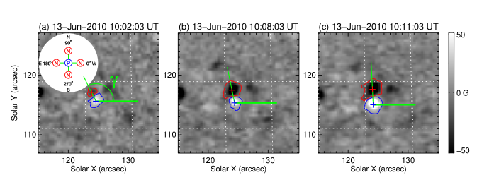
Figure 8: Sequence of magnetograms illustrating the rotation of an ER at the emergence stage. The contours, plus signs, and dotted curves have the same meanings as those in Figure 3. $\gamma$ is the orientation which varies between (0°, 360°). The definition of $\gamma$ is displayed in the inserted circular area in panel (a). “P” and “N” represent the positive and negative polarities, respectively.

We produce movies with the HMI magnetograms firstly, and then try our best to carefully examine them by eyes. ERs are identified as dipolar patches with opposite polarities emerge simultaneously or one following the other, and then grow and separate. Each ER is identified and tracked by eyes, which makes our results are very reliable. We define the time when both the positive and the negative patches are detected as the start time (t₀) of the emergence. If the strength of a magnetic patch exceeds the noise level, 10.2 Mx cm^-2 (Liu et al. 2012), we consider it as being detected. When the total unsigned magnetic flux of the two polarities reaches the maximum, the time is defined as the end time (t₁) of the emergence stage. The ER area is calculated from the pixels occupied by the magnetic fields stronger than the noise level. The separation distance is measured along the great circle on the solar surface between the magnetic centroids of positive and negative patches. Similar to the separation distance, the shift distance is also calculated on the sphere, but between the magnetic centroid of the entire ER at t₀ and that at t₁. The definition of ER’s orientation angle $\gamma$ is illustrated in the inserted circular area in Figure 8(a). “P” and “N” represent the magnetic centroids of ER’s positive and negative polarities, respectively. $\gamma$ is defined as the azimuth of “P–N” in the heliographic coordinate, where the west is 0$\arcdeg$ and the north is 90$\arcdeg$, instead of in the Cartesian coordinate. The range of $\gamma$ is (0$\arcdeg$, 360$\arcdeg$). The flux emergence rate, separation velocity, shift velocity, and angular speed of rotation are the average values during emergence.

3 RESULTS

3.1 Latitudinal distribution and magnetic flux of ERs

In the target delineated by the blue curve (see Figure 1), we identified 2988 ERs in all. After projection correction, the real area of our target outlined by the blue curve in Figure 1 is 8.0 $\times$ 10⁵ Mm², and thus the average number density in the whole target is 9.32 $\times$ 10^-4 day^-1 Mm^-2. This value is larger than that (8.7 $\times$ 10^-4 day^-1 Mm^-2) determined by Wang (1988) and that (6.7 $\times$ 10^-4 day^-1 Mm^-2) determined by Martin (1989), while it is smaller than those (17 $\times$ 10^-4 day^-1 Mm^-2, 27 $\times$ 10^-4 day^-1 Mm^-2, 71 $\times$ 10^-4 day^-1 Mm^-2) determined by Chae et al. (2001), Harvey (1993), and Hagennar (2001), respectively. The different values of average number density are marked with dashed horizontal lines in Figure 2(a). In our opinion, different data from different instruments and different sample sizes may lead to the difference of the results. The latitudinal distribution of these ERs is presented in Figure 2(a). The ERs are not uniformly distributed in the range of (S60$\arcdeg$, N60$\arcdeg$). There are two regions with larger number density: one is located around S15$\arcdeg$ and the other one around N25$\arcdeg$. This appearance was also presented in the study of Hagennar et al. (2003). The number densities at these two regions exceed 10 $\times$ 10^-4 day^-1 Mm^-2, higher than the density (8.8 $\times$ 10^-4 day^-1 Mm^-2) at the equatorial region between S10$\arcdeg$ and N10$\arcdeg$. The regions with latitude higher than 40$\arcdeg$ have much lower density, only about (5 $\sim$ 6) $\times$ 10^-4 day^-1 Mm^-2. The probability density function (PDF) of the ERs with a bin size of 0.6 $\times$ 10¹⁸ Mx is plotted in Figure 2(b). We can see that there is a PDF peak at 3.6 $\times$ 10¹⁸ Mx, and the mean magnetic flux is 9.27 $\times$ 10¹⁸ Mx. This value is close to the results of Hagenaar (2001; 1.13 $\times$ 10¹⁹ Mx), Schrijver et al. (1998; 1.3 $\times$ 10¹⁹ Mx), and Wang (1988; 1.5 $\times$ 10¹⁹ Mx), but it is not well consistent with several other results (2.5 $\times$ 10¹⁹ Mx, Martin 1989; 2.8 $\times$ 10¹⁹ Mx, Chae et al. 2001; 3.3 $\times$ 10¹⁹ Mx, Harvey 1993; 3.9 $\times$ 10¹⁹ Mx, Zhao & Li 2012), especially the very early study ($\sim$ 10²⁰ Mx) by Harvey & Martin (1973). The mean values reported by different studies are marked with dashed vertical lines in Figure 2(b). This difference may be due to the better sensitivity and higher spatial resolution of SDO/HMI. Although Zhao & Li (2012) also used HMI data, they only selected large ERs, so they obtained a higher ER magnetic flux. Wang et al. (2012) investigated ERs using Hinode data with high spatial resolution, however they just focused on IN ERs. They found that the IN ERs have magnetic fluxes from several 10¹⁶ Mx to 1.5 $\times$ 10¹⁸ Mx, and the average flux is about 0.8 $\times$ 10¹⁸ Mx, more than one order of magnitude smaller than our result. The magnetic flux of the ERs spreads from smaller than 10¹⁸ Mx to larger than 10²⁰ Mx, but none of them is larger than 3 $\times$ 10²⁰ Mx, the upper limitation of ER flux defined by Hagenaar et al. (2003).

3.2 Separation and growth of ER’s opposite polarities

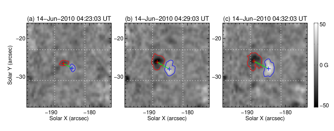
Figure 3: Sequence of HMI magnetograms illustrating the separation and growth of the dipolar patches of an ER at the emergence stage. The blue and red curves are contours of the ER’s positive and negative polarities at + 10.2 G and – 10.2 G levels, respectively. The blue and red plus symbols mark the magnetic centroids of the positive and negative polarities and the green curves are the distance between them along the great circle of solar surface. The dotted curves are the heliographic grids with a grid spacing of 0°.5.

The most conspicuous performance of ERs at the emergence stage is the separation and growth of dipolar patches. Figure 3 displays three magnetograms showing the separation and growth of the opposite polarities of an ER on 2010 June 14. The start time t₀ of the ER emergence was 04:23 UT. At that time, both of the positive (white patch with blue contour) and negative (black patch with red contour) polarities were strong enough to be detected (panel (a)). The total unsigned magnetic flux of the ER was 4.3 $\times$ 10¹⁷ Mx, the area occupied by the two patches was 2.7 Mm², and the mean absolute flux density was 15.9 Mx cm^-2. The distance (marked by the green curve) between the two magnetic centroids (indicated by the blue and red plus signs) was 1.9 Mm. Then 6 min later, the ER area expanded conspicuously, and the strength was much stronger compared with the initial appearance at the start time (panel (b)). At 04:32 UT, the total unsigned magnetic flux of the ER reached the maximum, 2.7 $\times$ 10¹⁸ Mx. According to the definition, it was the end time t₁, indicating the end of emergence. Thus, the duration of emergence was 9 min. The area expanded to 12.3 Mm², the mean flux density changed to 21.8 Mx cm^-2 and the separation distance reached 3.2 Mm. During the emergence period, the average separation velocity was 2.5 km s^-1 and the average flux emergence rate was 4.2 $\times$ 10¹⁵ Mx s^-1.

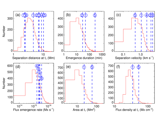
Figure 4: PDFs of separation distance (panel (a)) at t₁, emergence duration (panel (b)), separation velocity (panel (c)), flux emergence rate (panel (d)), area (panel (e)) at t₁, and flux density (panel (f)) at t₁. The values obtained by different studies are marked with dashed vertical lines: “1” (Present study), “2” (Schrijver et al. 1998), “3” (Chae et al. 2001), “4” (Hagenaar 2001), “5” (Zhao & Li 2012), “6” (Harvey & Harvey 1976), “7” (Wang et al. 2012), “8” (Title 2000), and “9” (Wang 1988).

The PDFs of separation distance at t₁, emergence duration, separation velocity, flux emergence rate, area at t₁, and flux density at t₁ are displayed in Figure 4. Each of them has a peak value. The separation distance ranges from 1.3 Mm to 19.2 Mm with a peak at 3.2 Mm, and the mean value is 4.7 Mm (panel (a)). The peak of the emergence duration is at 12 min, and the mean duration is 49.3 min (panel (b)). During the emergence, the separation velocities of ERs vary between 0.03 km s^-1 and 5.5 km s^-1, and their PDF peaks at 0.4 km s^-1 (panel (c)). The mean separation velocity is 1.1 km s^-1. The peak value and mean value of flux emergence rate are at 1.0 $\times$ 10¹⁵ Mx s^-1 and 2.6 $\times$ 10¹⁵ Mx s^-1, respectively (panel (d)). The areas at the end of emergence have a distribution peak at 10.0 Mm² and the mean area is 23.1 Mm² (panel (e)). The magnetic flux densities of the ERs are also determined at the end of emergence. Most ERs are not strong, only several ten Mx cm^-2, and the peak value of PDF is at 28.0 Mx cm^-2, as shown in panel (f). The mean flux density of ERs is 35.3 Mx cm^-2. Schrijver et al. (1998) found that the initial emergence phase lasts about 30 min, the separation distance is up to about 7 Mm, and the separation velocity is about 4 km s^-1 (marked with dashed vertical lines labeled with “2” in Figure 4). In the study of Hagenaar (2001), the average distance between the opposite polarities is 8.9 Mm and the expanding velocity is 2.3 km s^-1 (marked with lines “4”). As reported by Chae et al. (2001) and Harvey & Harvey (1976), the values of average separation of fully developed ERs are 7.4 Mm (marked with line “3”) and 2$-$3 Mm (line “6”), respectively. The separations of IN ERs obtained by Wang et al. (2012) are 3$\arcsec$$-$4$\arcsec$ and the average value is 3$\arcsec$.3, i.e., 2.4 Mm (line “7”). At the very beginning phase of emergence, the separation velocity determined by Title (2000) is of the order of 5 km s^-1 (line “8”). The mean flux emergence rates determined by Hagenaar (2001), Zhao & Li (2012), Harvey & Harvey (1976), and Wang (1988; line “9”) are 1.6 $\times$ 10¹⁵ Mx s^-1, 2.31 $\times$ 10¹⁵ Mx s^-1, 3.4 $\times$ 10¹⁵ Mx s^-1, and 2.2 $\times$ 10¹⁵ Mx s^-1, respectively. Their results are generally consistent with ours. However, there are also some differences which may be due to different observations. According to the results (vertical lines labeled with “5”) of Zhao & Li (2012), the values of some parameters (such as unsigned flux, duration, distance, and area) are consistent with these with large magnetic flux in our study, since they selected their sample with three criterions, and thus small ERs were ignored. According to the results of Harvey (1993), the lifetime of ERs is 4.4 hr. The emergence duration determined in the present study is about 50 min, so the birth stage is only about 0.19 of the lifetime.

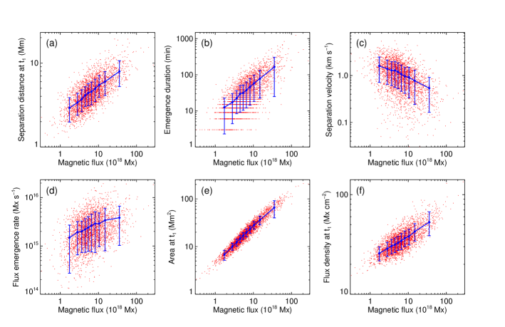
Figure 5: Scatter plots of separation distance, emergence duration, separation velocity, flux emergence rate, area, and flux density versus magnetic flux of ERs (red symbols) and of sorted and grouped points (blue symbols) (from panel (a) to panel (f), respectively). Each error bar represents the standard deviation of the corresponding group data.

Figure 5 shows the relationships between the parameters mentioned above and the total unsigned magnetic flux of ERs. The red dots are the scatter plots of all the ERs. In order to well display the relationships, the data are processed with a “sort-group” method (Zhao et al. 2009). Firstly, the data are sorted in ascending order according to the total unsigned flux. Then each 300 ERs are grouped into one group, and 10 groups are obtained in all. Finally, the parameters are correlated with the magnetic flux, and the values of ten groups are plotted (marked by the blue symbols in each panel). Each error bar represents the standard deviation of the corresponding group data. We can see that the separation distance (panel (a)), emergence duration (panel (b)), flux emergence rate (panel (d)), area (panel (e)), and flux density (panel (f)) are positively correlated with the magnetic flux. While the separation velocity has a negative correlation with the magnetic flux (panel (c)). The variation trends indicate that, the higher the total unsigned magnetic flux is, (1) the further the two polarities separate, (2) the longer the emergence last, (3) the slower the separation is, (4) the higher the flux emergence rate is, (5) the larger the area is, and (6) the stronger the ER field is. Harvey & Harvey (1976) have found that the flux emergence rate is large for the larger ERs, and Zhao & Li (2012) showed that the emergence duration and flux growth rate are positively correlated to the total emerging flux, which are supported by our results (see Figures 5(b) and 5(d)).

3.3 Shift of ER’s magnetic centroid

We also compute the magnetic centroid of each ER using its total unsigned magnetic flux. During the emergence, the magnetic centroid does not keep stable, and there exists a shift on the solar surface. Figure 6 shows the evolution of an ER as an example to illustrate this kind of movement. At 00:44 UT on June 12, the ER emergence began (panel (a)). The ER centroid was marked by the green plus symbol, and it was located at ($-$6.$\arcsec$5, 19.$\arcsec$1). At 00:53 UT, the location of magnetic centroid moved to ($-$7.$\arcsec$3, 18.$\arcsec$6), indicating that the ER moved in a south-east direction (panel (b)). When the emergence ended, the ER reached to ($-$8.$\arcsec$2, 17.$\arcsec$4) (panel (c)). The shift movement relative to the heliospheric grids can also be easily found. From t₀ to t₁, the centroid shifted 1.76 Mm in 54 min with an average shift velocity of 0.54 km s^-1.

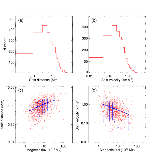
Figure 7: Upper panels: PDFs of shift distance (panel (a)) and shift velocity (panel (b)). Lower panels: Scatter plots of shift distance (panel (c)) and shift velocity (panel (d)) versus magnetic flux of ERs.

For the shift distance and shift velocity of ERs, their PDFs and their relationships with the total unsigned magnetic flux are presented in Figure 7. The shift distance is no more than several Mm, and the mean distance is 1.1 Mm while the peak value is at 0.4 Mm (panel (a)). The PDF of shift velocity peaks at 0.2 km s^-1 and the mean velocity is 0.9 km s^-1 (panel (b)). Similar to the relationship between the separation distance and the total unsigned magnetic flux shown in Figure 5(a), there is also a positive correlation for the shift distance as seen in Figure 7(c). The increase trend indicates that the higher the total magnetic flux is, the larger the shift distance is. The shift velocity is negatively correlated with the magnetic flux (panel (d)), indicating that the higher the total magnetic flux is, the slower the ER’s centroid shifts.

3.4 Orientation and rotation of ERs

Besides the separation movement and shift movement, ERs also rotate during the emergence, leading to the change of orientation. An example of ER rotation is given in Figure 8. At 10:02 UT on June 13, both the positive and negative polarities of the ER appeared. The initial orientation is shown in panel (a). The negative patch was located at the north-east of the positive patch, and the orientation was 113.$\arcdeg$1. Then the axis of the ER rotated clockwise, and 6 min later, the orientation changed to 101.$\arcdeg$1 (panel (b)), much smaller than the initial angle. The emergence went on, and the clockwise rotation also did not stop. At the end of of emergence, there was a significant change of the ER appearance (panel (c)). The orientation became 93.$\arcdeg$1, which means the ER rotated clockwise 20.$\arcdeg$0 with an absolute average angular speed of 2.$\arcdeg$2 min^-1 at the emergence stage.

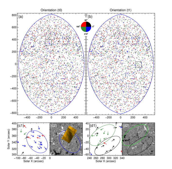
Figure 9: Spatial distribution of the ER orientations at the start time (panel (a)) and the end time (panel (b)) of flux emergence. Panel (c1) is the enlarged frame outlined by the square in panel (a), and panel (c2) is the corresponding magnetogram. Panels (d1) and (d2) are similar to panels (c1) and (c2) but for the area outlined by the square in panel (b). The inserted colorful image in panel (c2) is the AIA 171 Å observation and displays the overlying coronal loops (emphasized with dotted green curves) between positive and negative magnetic fields. The ellipses outline the ERs which are generally ordered.

Due to the rotation, the orientations of ERs at t₀ and at t₁ are different. Figure 9 displays the spatial distribution of the orientations at the start time (panel (a)) and the end time (panel (b)) of flux emergence. In the whole target, the orientations both at t₀ and t₁ are randomly distributed, but in some sizable (100$\arcsec$ $\times$ 100$\arcsec$) areas, ERs are generally ordered. For example, as shown in panel (c1), the orientations of ERs outlined by the ellipse are mainly from the positive to the negative polarities (see panel (c2)). The inserted colorful image in panel (c2) is the AIA 171 Å observation and displays the overlying coronal loops (emphasized with dotted green curves) between positive and negative magnetic fields. In panel (d1), the general pointing directions of the ERs located within the green circle are from northwest to southeast, consistent with the alignment of positive and negative polarities of the large-scale background fields (see panel (d2)). The black circle in panel (d1) contains ERs which mainly align in the southeast–northwest direction, also the direction of background fields, as shown in panel (d2). These results imply that, in some sizable areas, ER orientation may depend on the large-scale magnetic configuration.

The histograms of the orientations at t₀ and those at t₁ are presented in the left and the right columns in Figure 10, respectively. The histograms are shown in angular representation with a bin size of 45$\arcdeg$, and the ERs located in the northern and southern hemispheres are separately considered. At the start time of emergence, the initial orientations are essentially randomly distributed for both the northern (panel (a)) and southern (panel (b)) ERs. At the end of emergence stage, the orientations after rotation are still basically randomly oriented in the northern hemisphere, also in the southern hemisphere.

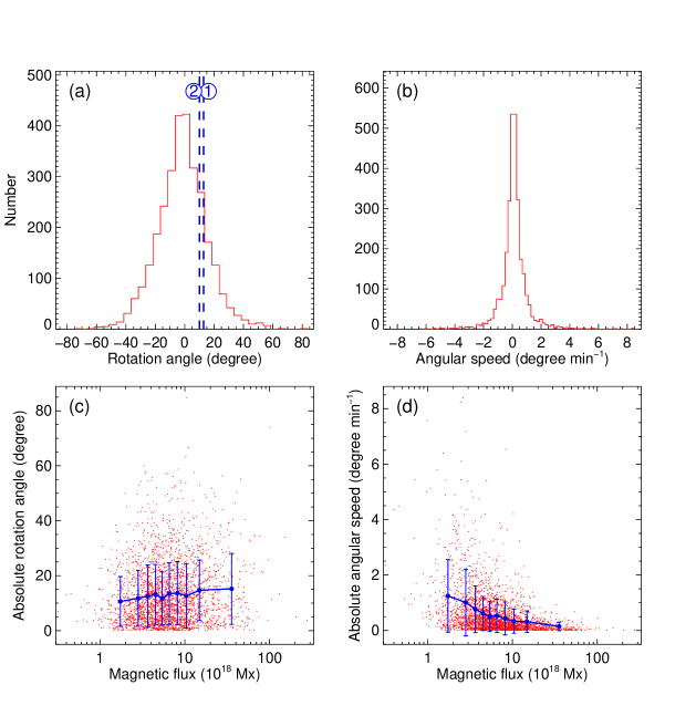
Figure 11: Upper panels: PDFs of rotation angle (panel (a)) and angular speed (panel (b)). Lower panels: Scatter plots of absolute rotation angle (panel (c)) and absolute angular speed (panel (d)) versus magnetic flux of ERs. Different values obtained by the present study and Wang et al. (2012) are marked with dashed lines “1” and “2”, respectively.

Figure 11 shows the PDFs of rotation angle and angular speed, and their relationships with the magnetic flux. If one ER rotates anticlockwise, its rotation angle and angular speed are assigned a plus, and if it rotates clockwise, a minus is assigned. The PDF of rotation angle have a general balance between the positive and negative values, and the peak is at zero (panel (a)). The mean value of absolute rotation angles is 12$\arcdeg$.9 (marked with line “1”). This value agrees with that ($>$ 10$\arcdeg$; marked with line “2”) of IN ERs reported by Wang et al. (2012). The data of angular speed also peak at zero, and the mean absolute angular speed is 0$\arcdeg$.6 min^-1 (panel (b)). The plots in panel (c) show that there is no close relationship between absolute rotation angle and magnetic flux, i.e., the rotation angle does not depend on the magnetic flux. The variation of absolute angular speed with magnetic flux is presented in panel (d). The decrease trend reveals that the higher the magnetic flux is, the lower the absolute angular speed is.

Some ERs rotate clockwise, while some anticlockwise. In Figure 1, the red dots represent the ERs with anti-clockwise rotation, while the blue ones represent the ERs with clockwise rotation. In order to examine if there exists a hemisphere rule for the ER rotation, the ERs at different latitudes should be considered separately. We define an imbalance parameter $\rho$ to describe the number imbalance between the anticlockwise and the clockwise rotated ERs. $\rho$ is defined as

$$\rho=\frac{N_{anticlockwise}-N_{clockwise}}{N_{anticlockwise}+N_{clockwise}},$$ (1)

where “N” is the ER number. The parameter $\rho$ as a function of latitude is shown in Figure 12. It shows that there is no significant domination of anticlockwise rotation or of clockwise rotation at different latitudes. The average value of $|\rho|$ is about 0.03 and the maximum value is smaller than 0.07.

4 CONCLUSIONS AND DISCUSSION

In this study, we have statistically investigated the properties of ERs. Based on almost three thousands of ERs, we quantitatively determine their parameters at the emergence stage for the first time. During the emergence process, there are three kinds of kinematic performances, e.g., separation of dipolar patches, shift of ER’s magnetic centroid, and rotation of ER’s axis. Several parameters, e.g., duration of emergence, flux emergence rate, and separation velocity, are measured. At the end of emergence, six parameters, i.e., magnetic flux, area, flux density, separation distance, shift distance, and rotation angle are also determined. Moreover, we find that the higher the ER magnetic flux is, (1) the further the two polarities separate, (2) the longer the emergence lasts, (3) the slower the separation is, (4) the higher the flux emergence rate is, (5) the larger the area is, (6) the stronger the ER field is, (7) the larger the shift distance is, (8) the slower the ER’s centroid shifts, and (9) the lower the absolute angular speed is. In addition, we notice that the regions with locations around S15$\arcdeg$ and around N25$\arcdeg$ have larger number density.

There are at least three kinds of convective cells according to their sizes, i.e., granulation, mesogranulation, and supergranulation (Simon & Leighton 1964; Rast 2003). The horizontal velocity of supergranular flows is determined to be about 0.3$-$0.5 km s^-1 (Leighton et al. 1962; Simon & Leighton 1964). Magnetic elements which emerge within the supergranular cells are advected toward to the supergranular borders with a velocity of about 0.4 km s^-1 (Zhang et al. 1998). However, as revealed by our results and also observed by Schrijver et al. (1998), the separation velocity of dipolar patches at the emergence stage is much larger. We suggest that, when magnetic flux tubes rise from below the photosphere, the $\Omega$$-$shaped tubes are mainly affected by the buoyant force and can be ejected into the atmosphere of the Sun with a high velocity, leading to a rapid separation of the positive and negative polarities. After the emergence stage, magnetic patches are mainly driven by horizontal supergranular flows, and thus the separation slows down. We also find that the average shift velocity (0.9 km s^-1) of the ERs is larger than that of the supergranular flows. It may be due to the existence of configuration asymmetry of ERs. When ERs emerge, the separation of dipolar patches is not symmetric, so the shifts are observed. Another possible interpretation is that the planes the flux tubes are located in are not vertical, i.e., there exits tilt angles relative to the solar radial direction. As soon as they rise and get through the photosphere, the flux tubes will become vertical, resulting in the magnetic centroid sideward shifts (see Figure 6). As shown in this study, ERs display a rotation of their axes. One possible reason is that the chaotic convective motions shear and distort the dipolar patches. Another illustration is that the rotation is caused by the relaxation of twisted ERs (Patsourakos et al. 2008), implying the structures of ERs are quite complicate.

The most popular model about the formation of active regions is that they are generated by a dynamo action at the bottom of the convection zone, where the tachocline is located (Dikpati & Gilman 2001; Mason et al. 2002). The tachocline is a transition layer of solar rotation, from the solid-body rotation of the radiative interior to the differential rotation of the convection zone (Kosovichev 1996). The large shear in the tachocline can form and store large scale fields, which will emerge through the solar surface due to buoyant force (Parker 1993). Active regions are aligned generally in the east-west direction with a few degrees because of the effect of Coriolis force during the emergence of flux tubes (Hale et al. 1919; Schmidt 1968). But for the ERs in our study, not only at the start time, but also at the end time, their orientations are basically randomly oriented in both the northern and the southern hemispheres (Figure 10). Besides, neither the anticlockwise rotated ERs, nor the clockwise rotated ones dominate the northern or the southern hemisphere (Figure 12). The locations of the ERs spread all over the target from S60$\arcdeg$ to N60$\arcdeg$ (see Figure 1). These results imply that, differing from active regions, it seems that ER flux is not generated by the global dynamo, and it may be generated by a local dynamo. However, small flux systems are greatly affected by convective motion below the solar photosphere and will eventually have random orientation when they emerge even if they may have been generated by the global dynamo. So we cannot exclude the possibility that they may be generated by the global dynamo. Figure 2(a) shows that, instead of the equatorial or the high latitudinal regions, the regions at around S15$\arcdeg$ and N25$\arcdeg$ (the general latitudes of active regions) have larger ER number density, indicating that the recycle of magnetic flux from decayed and dispersed active regions may be another origin of the magnetic flux of ERs.

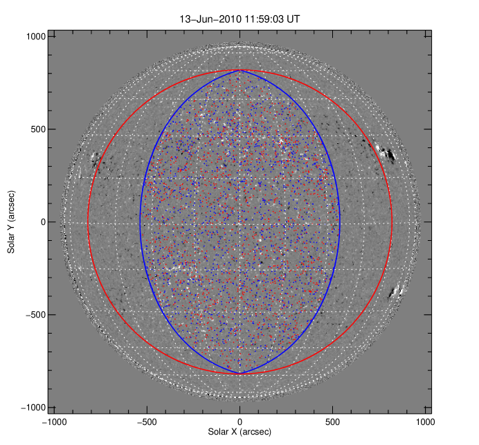
Figure 1: Distribution of the ERs. The background is the line-of-sight magnetogram observed by SDO/HMI at 11:59 UT on 2010 June 13. Each red/blue dot represents an ER with anti-clockwise/clockwise rotation. The red circle is located at the place with heliocentric angle $\alpha$ of 60°. The blue curve figures out the area where $\alpha$ $<$ 60° in the whole four days (June 11 12:00 UT – June 15 12:00 UT).

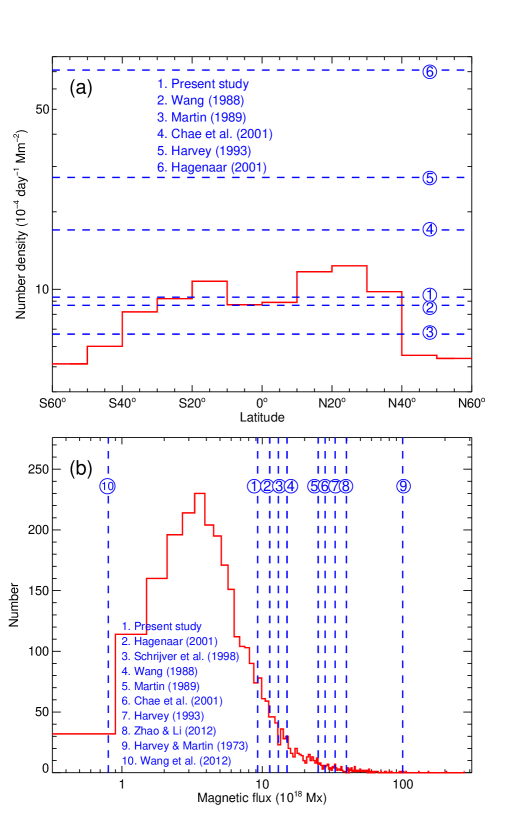
Figure 2: Upper panel: Number density of ERs as a function of latitude. Lower panel: PDF of total unsigned magnetic flux of ERs with a bin size of 0.6 $\times$ 10¹⁸ Mx. The dashed lines mark different values obtained by different studies.

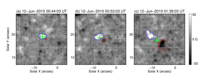
Figure 6: Sequence of magnetograms illustrating the shift of magnetic centroid of an ER at the emergence stage. The blue/red curves are contours of the ER’s positive/negative polarity at +/– 10.2 G, and the green plus symbols mark the magnetic centroid of the ER. The dotted curves are the heliographic grids with a grid spacing of 0°.5.

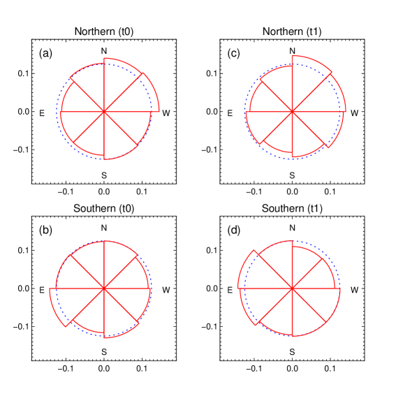
Figure 10: Histograms of the ER orientations at the start time (t0; left column) and the end time (t1; right column) of flux emergence in angular representation. The northern (upper panels) and the southern (lower panels) hemispheres are displayed separately. The dotted blue circles are shown as a reference if the ERs are definitely randomly oriented.

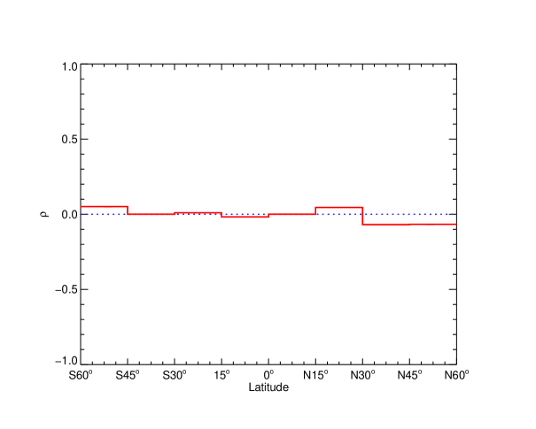
Figure 12: Number imbalance between anti-clockwise rotated and clockwise rotated ERs as a function of latitude.

References

- Cattaneo (1999) Cattaneo, F. 1999, ApJ, 515, L39
- Chae et al. (2001) Chae, J., Martin, S. F., Yun, H. S., et al. 2001, ApJ, 548, 497
- Dikpati & Gilman (2001) Dikpati, M., & Gilman, P. A. 2001, ApJ, 559, 428
- Hagenaar (2001) Hagenaar, H. J. 2001, ApJ, 555, 448
- Hagenaar et al. (2008) Hagenaar, H. J., De Rosa, M. L., & Schrijver, C. J. 2008, ApJ, 678, 541
- Hagenaar et al. (2003) Hagenaar, H. J., Schrijver, C. J., & Title, A. M. 2003, ApJ, 584, 1107
- Hale et al. (1919) Hale, G. E., Ellerman, F., Nicholson, S. B., & Joy, A. H. 1919, ApJ, 49, 153
- Harvey (1993) Harvey, K. L. 1993, Ph.D. Thesis, Rijksuniv. Utrecht
- (9) Harvey, K. L., & Harvey, J. W. 1976, Air Force Rep. AFGL-TR-76-0225, Part II, 35
- Harvey & Martin (1973) Harvey, K. L., & Martin, S. F. 1973, Sol. Phys., 32, 389
- Harvey et al. (1975) Harvey, K. L., Harvey, J. W., & Martin, S. F. 1975, Sol. Phys., 40, 87
- (12) Hoyng, P. 1992, in The Sun, ed. J. T. Schmelz & J. C. Brown (NATO ASI Ser. C. 373; Dordrecht: Reidel), 99
- Kosovichev (1996) Kosovichev, A. G. 1996, ApJ, 469, L61
- Leighton et al. (1962) Leighton, R. B., Noyes, R. W., & Simon, G. W. 1962, ApJ, 135, 474
- Lemen et al. (2012) Lemen, J. R., Title, A. M., Akin, D. J., et al. 2012, Sol. Phys., 275, 17
- Liu et al. (2012) Liu, Y., Hoeksema, J. T., Scherrer, P. H., et al. 2012, Sol. Phys., 279, 295
- Martin (1988) Martin, S. F. 1988, Sol. Phys., 117, 243
- Martin & Harvey (1979) Martin, S. F., & Harvey, K. H. 1979, Sol. Phys., 64, 93
- (19) Martin, S. F. 1989, in IAU Symp. 138, Solar Photosphere: Structure, Convection, and Magnetic Fields, ed. J. O. Stenflo (Dordrecht: Kluwer), 129
- Mason et al. (2002) Mason, J., Hughes, D. W., & Tobias, S. M. 2002, ApJ, 580, L89
- Nordlund et al. (1992) Nordlund, A., Brandenburg, A., Jennings, R. L., et al. 1992, ApJ, 392, 647
- Orozco Suárez et al. (2012) Orozco Suárez, D., Katsukawa, Y., & Bellot Rubio, L. R. 2012, ApJ, 758, L38
- Parker (1993) Parker, E. N. 1993, ApJ, 408, 707
- Patsourakos et al. (2008) Patsourakos, S., Pariat, E., Vourlidas, A., Antiochos, S. K., & Wuelser, J. P. 2008, ApJ, 680, L73
- Pesnell et al. (2012) Pesnell, W. D., Thompson, B. J., & Chamberlin, P. C. 2012, Sol. Phys., 275, 3
- Ploner et al. (2001) Ploner, S. R. O., Schüssler, M., Solanki, S. K., & Gadun, A. S. 2001, Advanced Solar Polarimetry – Theory, Observation, and Instrumentation, 236, 363
- Priest et al. (2002) Priest, E. R., Heyvaerts, J. F., & Title, A. M. 2002, ApJ, 576, 533
- Rast (2003) Rast, M. P. 2003, ApJ, 597, 1200
- Scherrer et al. (2012) Scherrer, P. H., Schou, J., Bush, R. I., et al. 2012, Sol. Phys., 275, 207
- Schmidt (1968) Schmidt, H. U. 1968, in IAU Symp. 35, Structure and Development of Solar Active Regions, ed. K. O. Kiepenheuer (Dordrecht: Reidel), 95
- Schou et al. (2012) Schou, J., Scherrer, P. H., Bush, R. I., et al. 2012, Sol. Phys., 275, 229
- Schrijver et al. (1998) Schrijver, C. J., Title, A. M., Harvey, K. L., et al. 1998, Nature, 394, 152
- Simon & Leighton (1964) Simon, G. W., & Leighton, R. B. 1964, ApJ, 140, 1120
- Simon et al. (2001) Simon, G. W., Title, A. M., & Weiss, N. O. 2001, ApJ, 561, 427
- Stein et al. (2003) Stein, R. F., Bercik, D., & Nordlund, Å. 2003, Current Theoretical Models and Future High Resolution Solar Observations: Preparing for ATST, 286, 121
- (36) Title, A. M. 2000, Philos. Trans. R. Soc. London A, 358, 657
- Wang (1988) Wang, H. 1988, Sol. Phys., 116, 1
- Wang et al. (2012) Wang, J. X., Zhou, G. P., Jin, C. L., & Li, H. 2012, Sol. Phys., 278, 299.
- Webb et al. (1993) Webb, D. F., Martin, S. F., Moses, D., & Harvey, J. W. 1993, Sol. Phys., 144, 15
- Yang et al. (2012) Yang, S. H., Zhang, J., Li, T., & Liu, Y. 2012, ApJ, 752, L24
- Zhang et al. (1998) Zhang, J., Wang, J., Wang, H., & Zirin, H. 1998, A&A, 335, 341
- Zhao & Li (2012) Zhao, J., & Li, H. 2012, RAA, 12, 1681
- Zhao et al. (2009) Zhao, M., Wang, J. X., Jin, C. L., & Zhou, G. P. 2009, RAA, 9, 933