A Parametric Modeling Approach to Measuring the Gas Masses of Circumstellar Disks

Abstract

The disks that surround young stars are mostly composed of molecular gas, which is harder to detect and interpret than the accompanying dust. Disk mass measurements have therefore relied on large and uncertain extrapolations from the dust to the gas. We have developed a grid of models to study the dependencies of isotopologue CO line strengths on disk structure and temperature parameters and find that a combination of ¹³CO and C¹⁸O observations provides a robust measure of the gas mass. We apply this technique to Submillimeter Array observations of nine circumstellar disks and published measurements of six well studied disks. We find evidence for selective photodissociation of C¹⁸O and determine masses to within a factor of about three. The inferred masses for the nine disks in our survey range from $0.7-6\,M_{\rm Jup}$, and all are well below the extrapolation from the interstellar medium gas-to-dust ratio of 100. This is consistent with the low masses of planets found around such stars, and may be due to accretion or photoevaporation of a dust-poor upper atmosphere. However, the masses may be underestimated if there are more efficient CO depletion pathways than those known in molecular clouds and cold cores.

1. Introduction

All sun-like stars form accompanied by rotationally supported disks of gas and dust, a natural consequence of the conservation of angular momentum during a gravitationally driven contraction over more than two orders of magnitude from molecular cloud cores to disk scales. Exoplanet surveys have now established that the most common end-state of these disks is planets, typically with sizes and masses substantially less than that of Jupiter (Howard, 2013). A key first step toward understanding the origin and diversity of exoplanetary systems, and thereby the formation of the Solar System, is measuring circumstellar disk properties. The most fundamental quantity is mass, as this sets the amount of available raw material for forming planets.

Disks form with an initial composition inherited from the interstellar medium (ISM) where the gas-to-dust mass ratio is 100 (Bohlin et al., 1978). Despite the dust being such a minor constituent, it is the most readily observed as it radiates over a continuum from infrared to millimeter wavelengths. The standard practice has been to convert this emission to dust mass and then to total disk masses by assuming an ISM gas-to-dust ratio, a large and uncertain extrapolation of two orders of magnitude. Whereas the validity of this assumption has been confirmed on very large scales in the case of molecular clouds, where alternative and independent mass estimates can be made (Dame et al., 2001), this is a major source of uncertainty for circumstellar disks. In particular, it is known that the dust grains grow from sub-micron to millimeter sizes and beyond (Dullemond & Dominik, 2005), and such large grains are both structurally and thermally decoupled from the gas (Kamp & Dullemond, 2004; D’Alessio et al., 2006).

Most of the gas in a giant planet-forming disk is expected to be molecular and relatively cool, $T<100$ K. Collisional energies are too low for the bulk constituent, H₂, to emit significantly so asymmetric molecules with large dipole moments best trace the gas. HD is the closest chemical counterpart and was observed with far-infrared spectroscopy by the Herschel Space Observatory in the closest known, gas-rich, disk around TW Hydra (Bergin et al., 2013). As Herschel is no longer operating, additional disk mass measurements using this technique are not possible. CO is the most abundant molecule after H₂ and its millimeter wavelength rotational lines are the strongest that are observable from the ground (Thi et al., 2004; Dent et al., 2005). The CO lines are optically thick, however, and therefore an unreliable measure of mass. Even ¹³CO lines may have significant optical depth (Dutrey et al., 1996; van Zadelhoff et al., 2001) but are less saturated and, together with constraints on C¹⁸O, provide a means to more accurately measure the total number of molecules, as has been previously carried out for molecular clouds and cores (Goldsmith et al., 1997).

In this paper, we use Submillimeter Array (SMA) observations of the $J=2-1$ transitions of CO, ¹³CO, and C¹⁸O to constrain the gas masses of nine circumstellar disks in the nearby Taurus cloud. To analyze these data, we develop a parametric model of disk gas density, temperature, and chemistry to produce a large grid of CO isotopologue line luminosities. We find that the luminosity of low lying rotational transitions of ¹³CO and C¹⁸O correlate with gas mass and that we can determine its value to within at least an order of magnitude from combinations of the two. Although this is not as direct as the oft-used formulaic approach to measuring dust masses, this model grid approach provides a simple but robust way to measure of the gas content of circumstellar disks that is suitable for interpreting CO isotopologue line surveys in the future.

The observations are presented in §2. The modeling is described in §3, and we discuss general insights regarding the CO emitting region in disks and the utility of CO isotopologue lines for measuring disk masses. We apply the parametric model grid to published observations of well studied disks and the SMA survey in §4. Assuming that the CO-to-H₂ abundance is the same in disks as in molecular clouds and cores, we find that the surveyed disks all have low masses and lower gas-to-dust ratios than the ISM. We discuss possible explanations and implications in §5, and conclude in §6.

2. Observations

We observed nine Class II disks in the Taurus star forming region. This is one of the closest regions containing many young stars and has been extensively studied (Güdel et al., 2007). The sources are all optically visible, single stars of spectral type K or M, with large photospheric excesses at all infrared wavelengths, indicative of full dusty disks extending from the dust sublimation radius outwards. Based on their luminosity and effective temperature, the inferred stellar masses and ages are $\sim 0.6-0.7\,M_{\odot}$ and $\sim 1-3$ Myr, respectively.

The observations were carried out with the SMA on Maunakea, Hawaii. The array consists of eight 6-m antenna configured variously in compact and extended configurations to provide projected baselines ranging from 5 m to 240 m. Observations were carried out over 19 nights from November 2010 to January 2013, in moderately dry weather conditions with precipitable water vapor levels ranging from 1 mm to 4 mm, corresponding to zenith atmospherical optical depths of $0.05-0.15$ at the observing frequency of 230 GHz (1.3 mm wavelength). A table of observational details is provided in Appendix A.

The correlator was configured to place the $J=2-1$ lines of C¹⁸O and ¹³CO in the lower sideband, and CO in the upper sideband. High frequency resolution windows, consisting of 512 channels of width 203 kHz, were placed around these line frequencies to provide a velocity resolution of 0.28 ${\rm km~{}s^{-1}}$. The cumulative continuum bandwidth away from the lines was 3.5 GHz, which provided high dust mass sensitivity.

The observations for any given night cycled through between 2 and 4 sources and two gain calibrators (3C111, J0510+180) each half hour. This provided sufficient calibration of the atmospheric amplitude and phase variation and a wide range of spatial frequencies for each source to provide high image fidelity. The absolute flux scale was determined by observations of an unresolved or at most marginally resolved planet or giant planet satellite, variously Uranus, Callisto, or Titan. Based on the variation of the amplitude calibration and flux calibration measurements, we estimate the uncertainty on the source flux densities to be 20%.

Images were produced from the calibrated visibilities using standard inversion and cleaning procedures. The typical resolution (beamsize) of the final maps was $1\farcs 2\times 0\farcs 9$ for the uniformly weighted continuum maps and $\sim 50$% larger for the naturally weighted line maps, the choice of weighting based on the signal-to-noise in the data. Figure 1 presents the continuum and velocity integrated line maps for each source.

Whereas the continuum and CO emission are strongly detected in all sources, and generally resolved, the much weaker ¹³CO and C¹⁸O lines were not detected with sufficient dynamic range to study their spatial structure. However, we found that we can determine gas masses accurately from their integrated emission alone. The integrated line intensities and rms noise levels for the continuum and velocity integrated line maps are tabulated in Table 1. In the case of a non-detection, we use the detected line, ¹³CO where possible else CO, to define the spatial and velocity range over which to calculate the ($3\sigma$) upper limit to the emission.

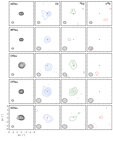
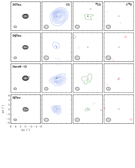
Figure 1.— SMA maps of the continuum and integrated line intensities for the nine Taurus disks in the survey. The black contours on the left hand side of each panel show the continuum emission with contours beginning at 5 mJy beam^-1 and increasing in multiples of 1.5. The integrated line maps have colored contours, blue for CO, green for ¹³CO, and red for C¹⁸O. The contours are linear beginning at and increasing in steps of three times the rms noise level, $\sigma$, listed in Table 1. The hashed ellipse shows the beamsize for each map in the lower left corner.

Table 1SMA 1.3 mm fluxes

	$F_{\rm cont}$ (mJy)		$F_{\rm CO}$ (Jy ${\rm km~{}s^{-1}}$)		$F_{\rm{}^{13}CO}$ (Jy ${\rm km~{}s^{-1}}$)		$F_{\rm C^{18}O}$ (Jy ${\rm km~{}s^{-1}}$)
Source	Value	$\sigma$	Value	$\sigma$	Value	$\sigma$	Value	$\sigma$
AA Tau	54.8	0.7	5.33	0.11	1.26	0.09	$<0.27$	0.09
BP Tau	42.5	1.0	1.11	0.08	$<0.24$	0.08	$<0.21$	0.07
CI Tau	152	1.1	2.51	0.13	2.70	0.13	$<0.39$	0.13
CY Tau	102	1.0	2.02	0.08	0.81	0.06	$<0.15$	0.05
DL Tau	164	1.1	1.98	0.12	0.43	0.06	$<0.15$	0.05
DO Tau	113	0.8	63.7	0.38	1.52	0.10	$<0.30$	0.10
DQ Tau	62.6	0.7	0.97	0.11	$<0.24$	0.08	$<0.21$	0.07
Haro 6-13	140	0.9	17.6	0.17	3.95	0.14	0.47	0.10
IQ Tau	57.6	1.0	2.52	0.08	0.48	0.07	$<0.21$	0.07

3. Modeling

Circumstellar disks are relatively small, faint objects that have, to date, required long integrations with millimeter wavelength interferometers to study their molecular gas content. Consequently, only a small number of disks have been imaged in isotopologue lines and most analyses have been tailored to the individual object. Driven by the moderately large sample size but low signal-to-noise level in our data here, we use a different approach. Rather than analyze each disk individually, we create a large grid of models that span a wide range of disk parameters, particularly in gas mass, and compare with the data in a uniform way. This approach is similar to the SED modeling of young stellar objects by Robitaille et al. (2006) and is also motivated by the grid modeling of mostly fine structure, far-infrared lines of atomic species for comparison with Herschel observations (Woitke et al., 2010; Kamp et al., 2011).

3.1. A parametric disk model

3.1.1 Density structure

The basic model for the gas structure is an exponentially tapered accretion disk profile in hydrostatic equilibrium (Williams & Cieza, 2011). This has its basis in the works of Hughes et al. (2008) and Andrews et al. (2009), who followed theoretical descriptions by Lynden-Bell & Pringle (1974) and Hartmann et al. (1998).

We define the azimuthally symmetric gas density $\rho(r,z)$ and temperature $T(r,z)$ in cylindrical coordinates. For a given temperature structure (see below), we can determine the shape of the vertical density structure by integrating the equation of hydrostatic equilibrium,

$$\frac{\partial\ln\rho}{\partial z}=-\left[\left(\frac{GM_{\rm star}z}{(r^{2}+z^{2})^{3/2}}\right)\left(\frac{\mu m_{\rm H}}{kT}\right)+\frac{\partial\ln T}{\partial z}\right],$$ (1)

where $\mu=2.37$ is the mean molecular weight of the gas and $m_{\rm H}$ is the mass of a hydrogen atom. The resulting vertical profile is normalized at each radius to have a vertically integrated surface density appropriate for an accretion disk around a central gravitating point source,

$$\Sigma(r)=\Sigma_{0}\left(\frac{r}{r_{c}}\right)^{-\gamma}\,\exp\left[-\left(\frac{r}{r_{c}}\right)^{2-\gamma}\right].$$ (2)

The global normalization is to the gas mass via

$$\Sigma_{0}=(2-\gamma)\,\frac{M_{\rm gas}}{2\pi r_{c}^{2}}\exp\left(\frac{r_{\rm in}}{r_{c}}\right)^{2-\gamma},$$ (3)

where $r_{\rm in}$ is the inner radius of the disk. We set this to 1 AU as the vast majority of the gas mass and of the CO millimeter emission is at large radii and this allows the computational resources to be concentrated on the outer disk. Our preliminary tests showed that the models are not sensitive to this value (as long as it is small).

For a given stellar mass, this prescription for the disk physical structure has three parameters; {$M_{\rm gas},r_{c},\gamma$}. Figure 2 plots all the surface density profiles in our model grid. These encompass the range inferred (and extrapolated from dust observations) for the most massive protoplanetary disks in Ophiuchus observed by Andrews et al. (2009) but extends to much lower masses, smaller sizes, and also includes flatter profiles.

To calculate the radiative transfer, we also require the velocity field, which we assume to be Keplerian with a Doppler width equal to the sum of a thermal and turbulent component,

$$v^{2}(r,z)=\frac{GM_{\rm star}}{(r^{2}+z^{2})^{1/2}},\hskip 18.06749pt\Delta v_{\rm D}^{2}(r,z)=\frac{2kT}{\mu m_{\rm H}}+\Delta v_{\rm turb}^{2}.$$ (4)

The prescription for the temperature is given below. The turbulent component is known to be subsonic (Hughes et al., 2011), and we fix its value at $\Delta v_{\rm turb}=0.01$ ${\rm km~{}s^{-1}}$.

The vertical profile and rotational speed also depend on the stellar mass and we include two values here, $M_{\rm star}=0.5,1\,M_{\odot}$ that bracket the range in our sample, to assess its effect on the CO line emission.

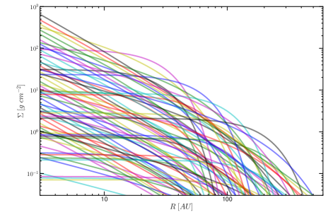
Figure 2.— The range of surface density profiles in the model grid for the range of parameters, {$M_{\rm gas},r_{c},\gamma$}, specified in Table 2.

3.1.2 Temperature structure

The disk temperature structure is purely parametric, but grounded in theory and observations. Deep in the disk, at $A_{\rm V}\lower 2.15277pt\hbox{$\;\buildrel>\over{\sim}\;$}10$ mag, the densities are sufficiently high for the gas and dust to be thermally coupled. Fits to continuum observations show that the radial midplane temperature gradient is a power law,

$$T_{\rm mid}(r)=T_{\rm mid,1}\left(\frac{r}{1\,{\rm AU}}\right)^{-q},$$ (5)

with typical values, $T_{\rm mid,1}\simeq 200$  K, $q\simeq 0.55$, for Taurus protostars similar to those in our CO survey (Andrews et al., 2009).

The temperature increases with height above the midplane due to heating from scattered stellar UV photons at $A_{\rm V}\simeq 1-10$ (Dullemond et al., 2002; D’Alessio et al., 2006; Lesniak & Desch, 2011). Furthermore, as the density decreases with increasing scale height, the gas and dust thermally decouple. Detailed models of the heating and cooling processes show the gas temperature smoothly transitions from the midplane value to a hotter atmospheric value at $z/r\sim 0.1-0.5$ for $r=10-100$ AU (Kamp & Dullemond, 2004; Nomura et al., 2007; Gorti & Hollenbach, 2008; Woitke et al., 2009). The uppermost disk surface layer, at $A_{\rm V}\lower 2.15277pt\hbox{$\;\buildrel<\over{\sim}\;$}0.1$ mag, may be superheated to still higher temperatures but CO molecules would not survive dissociation at such low column densities and we do not include this feature in our models.

Following Dartois et al. (2003), we parameterize the atmospheric temperature as a radial power law in the same way as for the midplane profile,

$$T_{\rm atm}(r)=T_{\rm atm,1}\left(\frac{r}{1\,{\rm AU}}\right)^{-q}.$$ (6)

As with Rosenfeld et al. (2013a), however, we use a sine instead of cosine function in the connecting function between the midplane and atmosphere so as to better match the vertical gas temperature profiles with the above mentioned models,

$$T(r,z)=\begin{cases}T_{\rm mid}+(T_{\rm atm}-T_{\rm mid})\left[\sin\left(\frac{\pi z}{2z_{q}}\right)\right]^{2\delta}&\mbox{if }z<z_{q}\\ T_{\rm atm}&\mbox{if }z\geq z_{q}\end{cases}.$$ (7)

This introduces two new parameters, $\delta,z_{q}$, that describe the steepness of the profile and the height at which the disk reaches the atmospheric value. We fix $\delta=2$ as this provides a good approximation to the gradient of the aforementioned theoretical models, and $z_{q}=4H_{\rm p}$ where $H_{p}$ is the pressure scale height derived from the midplane temperature, $(kT_{\rm mid}r^{3}/GM_{\rm star}\mu m_{\rm H})^{1/2}$, based on the level at which the optical depth to UV photons becomes unity (Lesniak & Desch, 2011). These same values were also used by Dartois et al. (2003) and Rosenfeld et al. (2013a). We run the full grid for these fixed values but investigate their effect on the line luminosities in Appendix B. There we show that they do not significantly affect our conclusions or mass estimates drawn from the full grid.

This prescription for the disk temperature structure has three parameters; {$T_{\rm mid,1},T_{\rm atm,1},q$} and a dependence on stellar mass through $z_{q}$. Figure 3 plots all the temperature profiles in our model grid for two radii. These profiles bracket the range and have a similar form as the aforementioned theoretical results. Although our focus here is on T-Tauri stars, these profiles are also sufficiently broad to encompass much of the expected range for Herbig Ae stars (Jonkheid et al., 2007).

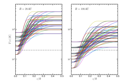
Figure 3.— The range of vertical temperature density profiles at radii of 20 AU (left panel) and 100 AU (right panel) in the model grid for the range of parameters, {$M_{\rm star},T_{\rm mid,1},T_{\rm atm,1},q$}, specified in Table 2. The horizontal dashed line is the CO freeze-out temperature, 20 K.

3.1.3 CO chemistry

CO has a relatively simple chemistry that is readily incorporated into our parametric model. CO forms quickly in the gas phase and uses up all the available carbon (van Dishoeck & Black, 1988). It is a very stable molecule with just two main destruction mechanisms, freeze-out onto dust grains at low temperatures near the disk midplane and photo-dissociation in the upper disk atmosphere. These have each been well characterized through several detailed studies.

CO depletion via freeze-out onto dust grains was first characterized in molecular cores (Caselli et al., 1999; Tafalla et al., 2002; Jørgensen et al., 2002), then inferred in circumstellar disks (Qi et al., 2008, 2011), and now directly resolved (Rosenfeld et al., 2013a). The resulting CO “snowline” also manifests itself in the enhanced abundance of N₂H⁺ and DCO⁺ (Qi et al., 2013; Mathews et al., 2013). From these results, we parameterize the freeze-out region as being at temperatures, $T<20$ K.

Energetic radiation from the central star and the interstellar radiation field dissociate CO in the upper layers of the disk. This results in a sharp transition from C to CO that we set to a column density, $N_{\rm dissoc}=1.3\times 10^{21}\,{\rm H}_{2}$ cm^-2 based on theory by Visser et al. (2009) and observations by Qi et al. (2011).

Consequently, a warm molecular layer, with nearly constant CO abundance, lies between the depleted midplane and dissociation surface (Aikawa et al., 2002; Woitke et al., 2009). Our models incorporate these results as follows,

$$x({\rm CO})={\rm[CO]/[H_{2}]}=\begin{cases}1\times 10^{-4}&\mbox{$T>20\,{\rm K},N_{\rm H_{2}}>N_{\rm dissoc}$}\\ 0&\mbox{elsewhere.}\end{cases}$$ (8)

An example disk density and temperature structure is shown in Figure 4. The CO emitting region that we observe with our millimeter wavelength observations is outlined by the black contours.

The isotopologues, ¹³CO and C¹⁸O, have the same freeze-out temperature as CO and will be depleted in the midplane. We therefore first model these species with the same density profile as CO but scaled by their respective isotopologue ratios, [CO]/[¹³CO]=70 and [CO]/[C¹⁸O]=550 (Wilson & Rood, 1994). These imply ¹³CO and C¹⁸O abundances relative to H₂ that are consistent with cloud measurements by Ripple et al. (2013) and Frerking et al. (1982) respectively.

The effect of photodissociation on the isotopologues is different than CO, however, as higher total column densities are required for these rarer species to self-shield. Visser et al. (2009) examined the complexities of this process, including the effects of dust, H, H₂, CO mutual shielding, excitation, doppler broadening, and ion-molecule isotope exchange reactions. They find that the [CO]/[¹³CO] ratio is relatively constant at the ISM value in disks with moderate grain growth but that C¹⁸O (and the rarer species, C¹⁷O and ¹³C¹⁸O) should decrease steadily to a factor of $\sim 7$ lower abundance relative to CO at high column densities toward the freeze-out region. The particular density profile of C¹⁸O within the warm molecular layer at intermediate column densities, $A_{\rm V}\simeq 1-10$ mag, is therefore a computationally complex function of both radius and height. To minimize the number of additional parameters, and in keeping with the simplicity of our approach, we approximate the effect of selective photodissociation by calculating a second set of C¹⁸O line intensities with the isotopologue abundance reduced by a factor of 3, [CO]/[C¹⁸O]=1650. The resulting two values, [¹³CO]/[C¹⁸O] $=8,24$, bracket recent observational results for molecular clouds in Orion (Shimajiri et al., 2014).

We emphasize that the model assumptions for the gas structure are only azimuthal symmetry and hydrostatic equilibrium. This allows us to consider fits to spectral line data independently from fits to continuum data and therefore to infer gas properties independently from those of the dust. This approach is necessary to match the reality of these two components being structurally, thermally, and dynamically decoupled. In particular, our constraints on gas masses are independent of dust mass measurements or, within the confines of our modeling parameters, any features in the dust structure such as inner holes or strong azimuthal features (van der Marel et al., 2013).

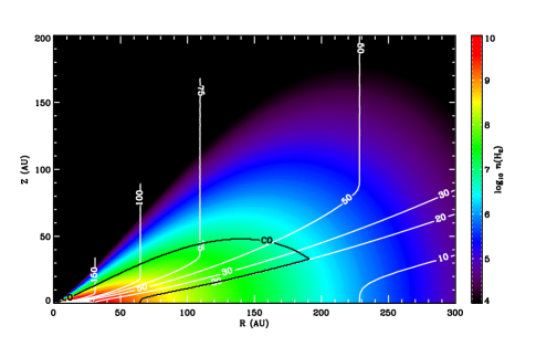
Figure 4.— The density and temperature distribution of a model disk. The star is at the origin and the disk is radially symmetric with mirror symmetry about the midplane at $Z=0$. The color scale represents the H₂ gas density on a logarithmic scale. The gas temperature is shown and labeled in the white contours. The black contours, labeled ‘CO’, represent the boundary of a warm molecular layer within which CO is expected to be in the gas phase and emit millimeter wavelength rotational lines. The parameters used for this model are $M_{\rm star}=1\,M_{\odot},M_{\rm gas}=0.01\,M_{\odot},R_{\rm c}=60\,{\rm AU},\gamma=0.75,T_{\rm mid,1}=200\,{\rm K},T_{\rm atm,1}=1000\,{\rm K},q=0.55$.

3.1.4 Radiative transfer

We calculate integrated line intensities for the models using the radiative transfer code RADMC-3D. The gas density, temperature, and CO abundance profiles were interpolated onto a spherical coordinate grid with 100 logarithmically spaced points in radial distance from 1 AU to 600 AU and 60 linear steps in polar angle, $\theta=10^{\circ}$ to $90^{\circ}$, with axial and mirror symmetry. We assumed Local Thermodynamic Equilibrium, which is a good approximation for the low lying CO rotational states at the densities and temperatures of the warm molecular region (Pavlyuchenkov et al., 2007).

The output is a set of data cubes of flux density, $F(x,y,\lambda)$, where $(x,y)$ is the projection on the sky in arcseconds for a distance to Taurus of 140 pc, and the wavelength $\lambda$ is chosen to cover the three lowest rotational transitions of CO, ¹³CO, and C¹⁸O, In principle, there is a tremendous amount of information available in these cubes for detailed modeling of resolved observations. However, because our ¹³CO and C¹⁸O observations do not have sufficiently high signal-to-noise ratios to study their spatial distribution, we spatially and spectrally integrated the model data cubes and use the line luminosities,

$$L=4\pi d^{2}\int F\,dx\,dy\,dv,$$ (9)

where $dv=cd\lambda/\lambda$ and $L$ has units Jy ${\rm km~{}s^{-1}}$ pc², to compare with the observations.

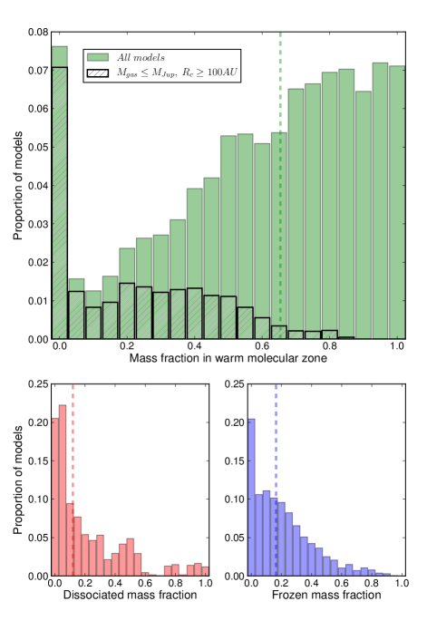
Figure 5.— The distribution of gas mass fraction in different regions of the disk for all the models in the grid. The top panel shows the mass fraction in the warm molecular layer, which is shielded from dissociation and is warm enough for CO to be in the gas phase. The dashed line shows the median of 65%. The hashed region shows that most of the models with low CO fractions are large, low mass disks. The lower panels show the distribution of the mass fraction in all models where CO is dissociated, $N({\rm H}_{2})<1.3\times 10^{21}$ cm^-2 (red histogram) and where it is frozen out, $T<20$ K (blue histogram). The dashed line in each panel indicates the median values, 12% and 16% respectively.

Table 2Parameter values of the model grid

Parameter	Range
$M_{\rm star}$	$0.5,1.0\,M_{\odot}$
$M_{\rm gas}$	$10^{-4},3\times 10^{-4},10^{-3},3\times 10^{-3},10^{-2},3\times 10^{-2},10^{-2}~{}M_{\odot}$
$r_{c}$	30, 60, 100, 200 AU
$\gamma$	0.0, 0.75, 1.5
$T_{\rm mid,1}$	100, 200, 300 K
$T_{\rm atm,1}$	500, 750, 1000, 1500 K
$q$	0.45, 0.55, 0.65
inclination	$0^{\circ},45^{\circ},90^{\circ}$
[CO]/[C18O]	550, 1650

3.2. Model grid

There are a total of nine parameters for each model, listed in the first column of Table 2. To explore the dependencies of the line intensities, we produced a grid of 18144 models that step through the set of values for each parameter listed in the second column. The stellar masses bracket those of the Taurus KM stars in our survey. The disk masses cover a wide range of gas masses from sub-Saturnian to above the minimum mass required to form the Solar System (Weidenschilling, 1977). The range for the surface density and temperature profiles are based on the discussion in §3.1.1 and §3.1.2 and illustrated in Figures 2 and 3 respectively. The three values for the viewing geometry (inclination) span the extremes of edge-on and face-on, with one intermediate.

We first calculated the mass fraction in those regions of the disk where CO is dissociated, $f_{\rm dissoc}$, and where it is frozen out, $f_{\rm freeze}$. These may overlap in very cold disks with low column densities, but in general there is a warm molecular layer where CO is in the gas phase with mass fraction, $f_{\rm CO}={\rm max}\{0,1-(f_{\rm dissoc}+f_{\rm freeze})\}$. Histograms of these fractions over the parameters in the grid are plotted in Figure 5. The median values for all disks are $f_{\rm dissoc}=12$%, $f_{\rm freeze}=16$%, and $f_{\rm CO}=65$%. The dissociation and freeze-out fraction both increase with the characteristic disk radius, $r_{c}$, as the outer regions are colder and of lower density. The freeze-out fraction is independent of disk mass as the temperature profile is specified independently and the disk mass only affects the scaling of the density but not its functional form. Lower mass disks have lower column densities, however, and therefore higher dissociation fractions. This can be a dominant factor for the very lowest mass disks but CO traces the bulk of the gas mass, $f_{\rm CO}>50$%, in 85% of disks with $M>M_{\rm Jup}$ for the models in our grid. These general results demonstrate the feasibility of using CO isotopologues for constraining gas masses, at least for disks with the capacity to form giant planets.

For each model disk, we calculate the line radiative transfer for CO, ¹³CO, and C¹⁸O at ISM abundances and for C¹⁸O at three times lower abundance to allow for selective photodissociation as discussed above. The line intensities of the different isotopologues generally follow each other but there is a large dispersion with CO on account of its very large optical depth. Furthermore, there are observational problems with using CO lines as cloud contamination can be severe (and indeed is directly seen in the SMA data for AA Tau, CI Tau, DO Tau and Haro 6-13). We therefore focus on the two isotopologues. Figure 6 plots the ¹³CO and C¹⁸O 2–1 line luminosities for all the models. The two lines strongly correlate with each other, with a median ratio, $L({\rm{}^{13}CO~{}2-1})/L({\rm C^{18}O~{}2-1})=3.2,7.0$, for [CO]/[C¹⁸O] $=550,1650$ respectively. As these median line ratios are only about half the abundance ratios, we infer that the optical depth in the ¹³CO line is significant. Nevertheless, disks with different masses tend to lie in different regions of this diagram. For any given mass, the dispersion in the line intensities is due partly to CO freeze-out and dissociation as well as excitation and optical depth.

Further examination of this plot shows that the line intensities are relatively insensitive to the disk inclination. This is because even edge-on disks present a large projected area due to their highly flared vertical structure (Beckwith & Sargent, 1993). For a given disk mass, the main factors that affect the line intensities are the temperature parameters, $T_{\rm atm,1}$ and $T_{\rm mid,1}$. Disks with high atmospheric temperatures have higher ¹³CO to C¹⁸O line ratios, i.e., they lie in the lower part of the envelope in Figure 6. This is likely due to a larger scale height and less saturation of the the ¹³CO line. The CO freeze-out fraction is higher in disks with cool midplanes and the intensities in both lines are correspondingly lower. The disk size, parameterized mainly by the characteristic radius, $r_{c}$, also broadens the dispersion with small disks tending to have lower intensities and lower ¹³CO to C¹⁸O line ratios. This is also likely an optical depth effect. However, low mass disks with large $r_{c}$ may also have low line intensities due to a high CO dissociation fraction.

The variation of the C¹⁸O abundance produces a corresponding change in the C¹⁸O line luminosity. There is also a greater dispersion in the models for any given mass for the lower C¹⁸O abundance, however, which suggests that the C¹⁸O emission from the disks with ISM abundances has a significantly optically thick component. Nevertheless, the change between the left and right panels of Figure 6 is almost orthogonal to the variation with mass so the impact on our ability to constrain gas masses is smaller than we might initially expect.

The combination of all these factors means that there are models that have the same line luminosity for disks that differ by as much as a factor of 30 in mass. Consequently, it is not possible to reliably measure the gas mass from the luminosity of a single line. However, the overlap in the two-dimensional scatter plot is much smaller, about a factor of 10 at most and typically one mass bin or a factor of 3. The combination of ¹³CO and C¹⁸O is therefore a much better diagnostic of gas mass. The observations are overplotted on the Figure and discussed below.

The driving philosophy behind the parametric model is to create a simple look-up table for comparison with basic observables in a way that allows quick, uniform analyses of large samples. The integrated intensities for the $J=3-2,2-1,1-0$ transitions of CO, ¹³CO, and C¹⁸O (for both relative abundances) are tabulated in Table 3, and available online for the 18144 models in the grid.

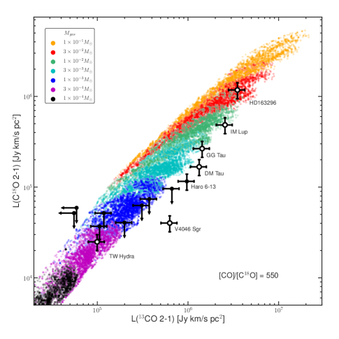
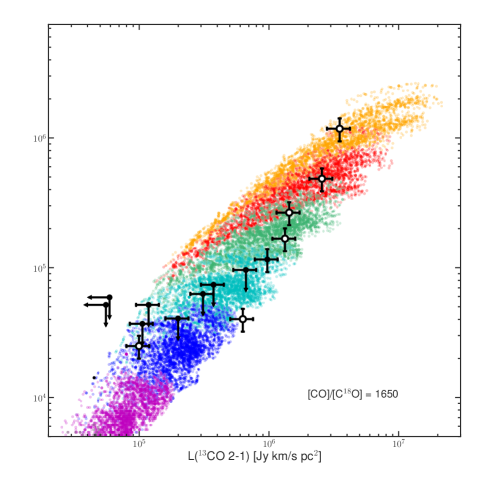
Figure 6.— Flux densities for the $J=2-1$ transitions of ¹³CO and C¹⁸O for the 18144 calculations in the model grid, color-coded by gas mass. There is a general trend of increasing flux density with increasing mass, but a given flux density of a single line can correspond to a very wide range of gas masses, about two orders of magnitude for ¹³CO, and an order of magnitude for C¹⁸O. The combination of both lines, however, allow a much more precise estimate of the gas mass, typically to within the factor of 3 model grid binning. The locations of the nine observed disks are noted in black and the labeled comparison disks in red.

Table 3Parametric Model Output

$M_{\rm star}$	$M_{\rm gas}$	$\gamma$	$R_{\rm c}$	$T_{\rm mid,1}$	$T_{\rm atm,1}$	$q$	$i$	$f_{\rm freeze}$	$f_{\rm dissoc}$	$F_{\rm CO1-0}$	$F_{\rm CO2-1}$	$F_{\rm CO3-2}$	$F_{\rm{}^{13}CO1-0}$	$F_{\rm{}^{13}CO2-1}$	$F_{\rm{}^{13}CO3-2}$	$F_{\rm C^{18}O1-0}$	$F_{\rm C^{18}O2-1}$	$F_{\rm CO^{18}3-2}$	$F_{\rm C^{18}O1-0}^{\rm low}$	$F_{\rm C^{18}O2-1}^{\rm low}$	$F_{\rm CO^{18}3-2}^{\rm low}$
($M_{\odot}$)	($M_{\odot}$)		(AU)	(K)	(K)		(∘)			(Jy ${\rm km~{}s^{-1}}$)	(Jy ${\rm km~{}s^{-1}}$)	(Jy ${\rm km~{}s^{-1}}$)	(Jy ${\rm km~{}s^{-1}}$)	(Jy ${\rm km~{}s^{-1}}$)	(Jy ${\rm km~{}s^{-1}}$)	(Jy ${\rm km~{}s^{-1}}$)	(Jy ${\rm km~{}s^{-1}}$)	(Jy ${\rm km~{}s^{-1}}$)	(Jy ${\rm km~{}s^{-1}}$)	(Jy ${\rm km~{}s^{-1}}$)	(Jy ${\rm km~{}s^{-1}}$)
0.5	1.00E-04	0	30	100	500	0.45	0	0.039	0.164	0.150	0.841	2.126	0.022	0.142	0.390	0.004	0.043	0.125	0.002	0.017	0.053
0.5	1.00E-04	0	30	100	500	0.45	45	0.039	0.164	0.158	0.835	2.043	0.023	0.162	0.452	0.005	0.045	0.133	0.002	0.018	0.055
0.5	1.00E-04	0	30	100	500	0.45	90	0.039	0.164	0.092	0.391	0.862	0.020	0.136	0.373	0.004	0.041	0.121	0.002	0.017	0.052
0.5	1.00E-04	0	30	100	750	0.45	0	0.029	0.169	0.212	1.407	3.862	0.020	0.152	0.455	0.004	0.039	0.122	0.001	0.015	0.048
0.5	1.00E-04	0	30	100	750	0.45	45	0.029	0.169	0.224	1.403	3.721	0.021	0.167	0.511	0.004	0.040	0.127	0.001	0.015	0.050

4. Results

The utility of the model grid is best demonstrated through application. Observations of ¹³CO and C¹⁸O 2–1 integrated line intensities for six well studied disks from the literature and for the sample of nine less well known but perhaps more typical disks from our SMA Taurus survey are overlaid on Figure 6. When detected, the measurements generally have a signal-to-noise ratio greater than 5 and the calibration uncertainty is greater than the measurement error. Aside from the numerous C¹⁸O upper limits in the case of the survey disks, therefore, we have placed error bars of $\pm 20$% on the data.

4.1. Comparison with well studied disks

A handful of disks have received more attention in the literature than others at millimeter wavelengths primarily due to their apparent brightness. That is, they are either relatively close or relatively massive. We found six disks with published results on the 2–1 lines of ¹³CO and C¹⁸O in the literature and compiled their integrated intensities in Table 4.

Table 4Comparison disk 1.3 mm fluxes

	$F_{\rm cont}$ (mJy)		$F_{\rm CO}$ (Jy ${\rm km~{}s^{-1}}$)		$F_{\rm{}^{13}CO}$ (Jy ${\rm km~{}s^{-1}}$)		$F_{\rm C^{18}O}$ (Jy ${\rm km~{}s^{-1}}$)		Dist.
Source	Value	$\sigma$	Value	$\sigma$	Value	$\sigma$	Value	$\sigma$	(pc)	Ref.
TW Hydra	540	30	17.5	1.8	2.72	0.18	0.68	0.18	54	1,2,3
V4046 Sgr	283	28	34.5	3.5	9.4	0.9	0.6	$\cdots$	73	4
DM Tau	109	13	14.9	0.4	5.40	0.13	0.68	0.07	140	6,7
GG Tau	593	53	21.5	1.6	5.82	0.19	1.08	0.10	140	6,7
IM Lup	195	$\cdots$	22.3	$\cdots$	5.65	$\cdots$	1.07	$\cdots$	190	8
HD 163296	670	0.7	54.17	0.39	18.76	0.24	6.30	0.16	122	5

With the exception of the Herbig Ae star, HD 163296, the stars in this sample have similar masses and luminosities as the low mass Taurus stars in our SMA survey. The range of temperatures in the model grid should therefore be appropriate for these systems. However, several of these disks are known to have inner cavities. This is particularly large in the case of the GG Tau binary system ($R\simeq 180$ AU, Dutrey et al., 1994), but also resolved in TW Hydra ($R\simeq 3$ AU, Menu et al., 2014; Hughes et al., 2007), DM Tau ($R\simeq 19$ AU, Andrews et al., 2011), and in the spectroscopic binary V4046 Sgr ($R\simeq 29$ AU, Rosenfeld et al., 2013b). The model grid does not incorporate large inner holes but since most of the mass lies at large radii for surface density profiles that are flatter than $\Sigma(r)\propto r^{-2}$ and because we are interested in low lying CO rotational lines that are readily excited in the outer parts, we expect the grid to be broadly applicable to these observations. Indeed we find that the ¹³CO and C¹⁸O line luminosities, while spanning a range of about a factor of 30, lie within our model results. The models with the reduced C¹⁸O abundance fit the data better in general which suggests that selective photodissociation is an important effect to consider in interpreting observations of this species.

Histograms of the gas masses that fit the ¹³CO line alone and the combination of ¹³CO and C¹⁸O (for any other model parameter) are shown in Figure 7. The inferred values range from below a Jupiter mass in the case of TW Hydra to above the MMSN for most others. The low mass inferred for the TW Hydra disk is consistent with detailed modeling of Herschel observations and CO and ¹³CO 3–2 lines (Thi et al., 2010) but notably discrepant with the HD mass measurement by Bergin et al. (2013). We discuss potential implications of this in §5. Dutrey et al. (1997) estimate masses for DM Tau and GG Tau based on modeling their chemistry that are consistent with our values. The Herbig Ae star, HD 163296 is the most massive and luminous star in the sample and has the most massive disk. It lies near the boundaries of our model grid parameters, which is designed to model T Tauri stars. Nevertheless, our inferred gas mass lies within a factor of two of the detailed modeling of multiple resolved CO and isotopologue lines by Qi et al. (2011).

There is no independent gas mass determination for IM Lup so we cannot compare with our results in this case. The only major discrepancy between our model grid results and detailed modeling of the CO lines in individual sources is V4046 Sgr where our estimated gas mass is significantly lower than a three-component model by Rosenfeld et al. (2013b). We note, however, that the C¹⁸O line was only marginally detected in that study and was not used to constrain their fits. The disk location in Figure 6 shows it to have an abnormally low C¹⁸O to ¹³CO line luminosity relative to other disks and very few models in our grid match both lines.

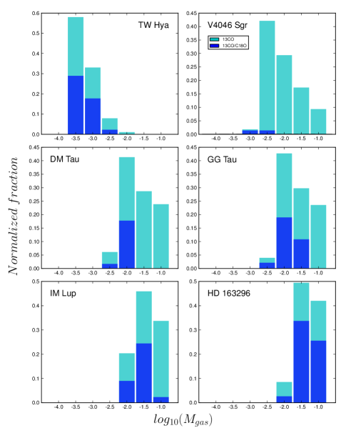
Figure 7.— The results of model grid fitting for gas masses for the six comparison disks listed in Table 4. Each panel is a histogram of the proportion of the models that match the observed line luminosities. The cyan histogram shows fits to the ¹³CO 2-1 line luminosity only and the blue is a subset that fits both the ¹³CO and C¹⁸O line luminosities. For each source, the histograms are normalized such that the cyan histogram sums to a total fraction of 1.

4.2. Fits to the surveyed disks

4.2.1 Case study: Haro 6-13

Haro 6-13 was the only disk in our SMA survey that was detected in C¹⁸O and therefore more tightly constrains the model parameters than the others. Figure 8 plots histograms of each of the nine parameters for fits to ¹³CO alone and for ¹³CO and C¹⁸O.

Considering the grid matches to the ¹³CO line alone shows a wide range in gas mass and all other parameters. This reiterates the expectation from from Figure 6 that a single line does not provide a strong constraint. Disks with gas masses that range over one order of magnitude match the line luminosity and the distribution of $f_{\rm freeze}$ is widely spreaad. As a moderately massive disk, however, the dissociation fraction $f_{\rm dissoc}$ is fairly small.

Fits to both the ¹³CO and C¹⁸O lines provide stronger constraints on the gas mass, to within a factor of 3 and somewhat less than the MMSN. The relatively weak C¹⁸O emission indicates a high [CO]/[C¹⁸O] ratio as expected for selective photodissociation. The histograms of the disk structure and temperature parameters do not show any strong preferences for particular values, which is simply a reflection that the gas mass is the primary determinant of the line intensities. This relative insensitivity means that unknowns such as the precise vertical temperature distribution are not strongly limiting factors in our ability to determine disk masses. A further important implication is the feasibility of this modeling approach for quantifying large surveys without specific detailed modeling of each individual system.

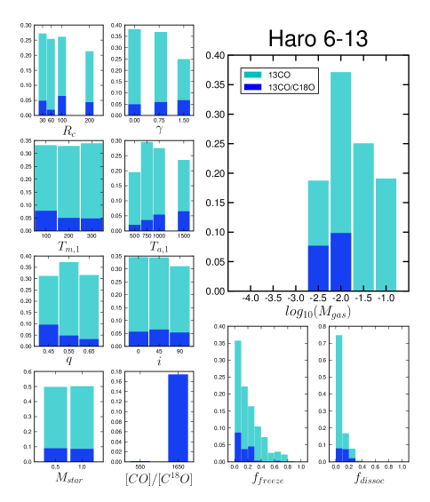
Figure 8.— Histograms of the nine parameters and the derived dissociated and frozen mass fractions for the models that match the Haro 6-13 observations to within 20%. The color coding and normalization is the same as in Figure 7.

4.2.2 The full survey

We have carried out the same exercise as above for the other eight disks in the SMA survey. Although C¹⁸O was not detected in any of these objects, we obtained sensitive upper limits that prove critical for constraining the gas masses, especially in the case of those sources with reasonably strong ¹³CO emission.

Figure 9 plots the histograms of the gas mass for the fits to the same line combinations as above. Models that range over a factor of 30 or more can match the ¹³CO line alone. The additional constraint from the C¹⁸O limit pins down down the mass range to about a factor of 3 for AA Tau, CI Tau, CY Tau, and DO Tau, and forces them to the lower range of the ¹³CO fits. This indicates that these disks are reasonably warm and have sufficient flaring that ¹³CO optical depth effects are not hiding a lot of mass. The inferred masses are low, $M_{\rm gas}\simeq 1-3\,M_{\rm Jup}$.

The information from the C¹⁸O line does not have the same leverage for the weaker sources DL Tau and IQ Tau and is inconsequential for the case of BP Tau and DQ Tau which were not detected even in ¹³CO (but the presence of CO demonstrates that some molecular gas exists). We conclude that these disks all have very low masses, $M_{\rm gas}\lower 2.15277pt\hbox{$\;\buildrel<\over{\sim}\;$}M_{\rm Jup}$. As with the histograms in Figure 8 for Haro 6-13, we find for all the disks that the low excitation CO isotopologue lines do not strongly constrain the other model parameters.

The primary result from this work is that the 9 Taurus disks in our survey all have low gas masses, well below the MMSN, and 5 have masses no greater than a Jupiter mass. This is surprising in that the masses are much lower than expected from the dust emission and implies low gas-to-dust ratios. It also has clear implications for planet formation and/or disk chemistry that are discussed in §5.

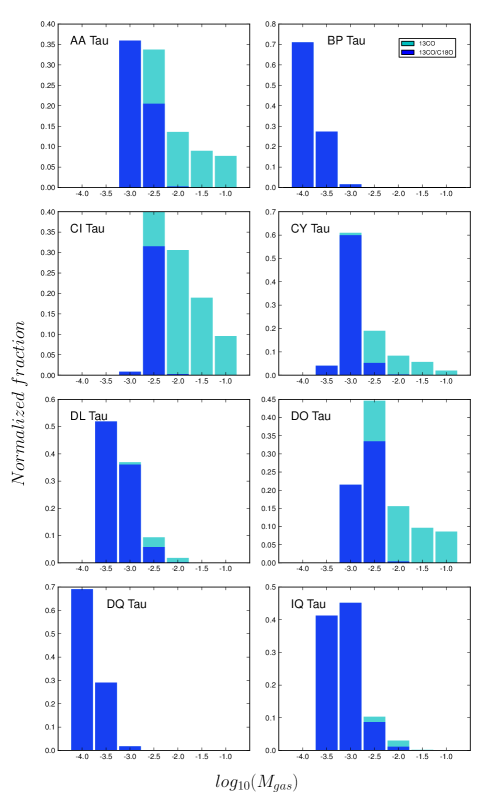
Figure 9.— The results of model grid fitting for gas masses for the eight other disks in the SMA survey. Each panel is a histogram of the proportion of the models that match the observed line luminosities. The color coding and normalization is the same as in Figure 7.

4.3. Dust masses and gas-to-dust ratios

For comparison with the gas masses from the model fits above, we calculated the dust masses using the standard equation,

$$M_{\rm dust}=\frac{F_{\rm cont}d^{2}}{\kappa_{\nu}B_{\nu}(T_{\rm dust})},$$ (10)

assuming optically thin emission and a constant temperature, $T_{\rm dust}$. Here $F_{\rm cont}$ is the continuum flux density listed in Tables 1 and 4, $d$ is the distance, $B_{\nu}$ is the Planck function at the observing frequency, $\nu$, and $\kappa_{\nu}=10(\nu/1000\,{\rm GHz}){\rm cm}^{2}\,{\rm g}^{-1}$ is the dust grain opacity from the prescription in Beckwith & Sargent (1991) without the implicit gas-to-dust ratio. Following Andrews et al. (2013) we scale the dust temperature with the stellar luminosity, $T_{\rm dust}=25(L_{\rm star}/L_{\odot})^{1/4}$ K. There are the well known caveats regarding the possibility of optically thick emission in the inner regions of the disk and missing mass in large grains (see, e.g., Williams & Cieza, 2011), and this measure of the dust mass is therefore a lower limit to the total mass of solids.

The derived gas and dust masses, and their ratios, are listed in Table 5 for the SMA survey and comparison disks. The gas masses here are weighted averages from the histograms in Figures 7, 8, 9. The range in dust masses is smaller than the range in gas masses which demonstrates that there is a significant dispersion in the gas-to-dust ratio. Figure 10 plots the gas masses with markers at the MMSN and Jupiter, and the gas-to-dust ratios with the fiducial ISM value of 100.

All the disks in the SMA survey and the two nearby comparison disks, TW Hydra and V4046 Sgr, have gas masses below the MMSN and gas-to-dust ratios below 100. Several have extremely low gas masses, comparable or below that of Jupiter, and all but Haro 6-13 have gas-to-dust ratios below 30. The comparison sample is biased toward bright objects and the more distant members, DM Tau, GG Tau, IM Lup, and HD 163296 are intrinsically massive. Their inferred gas masses are at the MMSN level or higher. Nevertheless, with the exception of HD 163296, these disks also have gas-to-dust ratios that are lower than 100.

The second main result from this work is that the gas-to-dust ratio is both low and varies widely from disk to disk. The mean ratio for the disks in the SMA survey is 16 with a standard deviation of 11. Including the comparison disks in addition, the mean is 25 with a standard deviation of 24. It appears that the composition of these Class II disks has evolved significantly from their initial conditions.

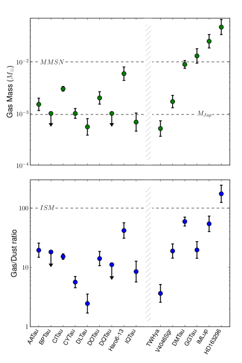
Figure 10.— The fitted gas masses and inferred gas-to-dust ratios for the nine Taurus disks in the SMA survey and the six comparison disks. The upper panel shows the mean gas masses with dashed lines at the Minimum Mass Solar Nebula ($0.01\,M_{\odot}$) and a Jupiter mass for comparison. Uncertainties are estimated from the range of the fits and the factor of 3 mass binning, except for the two sources, BP Tau and DQ Tau, which were undetected in ¹³CO and for which we can only determine upper limits. The lower panel is the ratio of gas mass to the dust mass derived from the continuum flux density, and is compared to the ISM value of 100 shown by the dashed line. The vertical hashes in each panel divide the SMA survey from the comparison disks as these are a more heterogeneous group in terms of stellar type and disk structure.

Table 5Gas and dust masses

Source	$M_{\rm gas}(10^{-4}\,M_{\odot})$	$M_{\rm dust}(10^{-4}\,M_{\odot})$	Ratio
AA Tau	15	0.77	19
BP Tau	$<10$	0.55	$<18$
CI Tau	30	2.0	15
CY Tau	10	1.8	6
DL Tau	5	2.2	2
DO Tau	20	1.4	14
DQ Tau	$<10$	0.90	$<11$
Haro 6-13	60	1.4	43
IQ Tau	7	0.80	9
TW Hydra	5	1.4	4
V4046 Sgr	17	0.90	19
DM Tau	90	1.5	60
GG Tau	130	6.6	20
IM Lup	250	4.6	53
HD 163296	470	2.7	170

5. Discussion

Given the small set of assumptions in our disk gas model and the wide range of parameters used to create the grid, it is not surprising that we are able to find model sets that match the observed integrated line intensities for each of the sources in Tables 1 and 4. It is more noteworthy, however, that the line intensities are more strongly dependent on mass than the parameters describing the disk density or temperature structure, at least for the range of expected, or in some cases observed, values. This then leads to the simple, but powerful, result that we can determine gas masses from the unresolved integrated emission of two lines reasonably accurately and independently of the details of their structure.

Our finding of low gas masses and low gas-to-dust ratios is somewhat unexpected. Hence it is worth noting that, even without detailed modeling, the observations here have line-to-continuum ratios $\sim 1-5$ for the ¹³CO 2–1 line, which is much lower than the observed values, $\lower 2.15277pt\hbox{$\;\buildrel>\over{\sim}\;$}100$ for star forming cores in NGC 1333 (Sun et al., 2006; Lefloch et al., 1998). In this basic observational sense, therefore, disks lie in a fundamentally different regime of parameter space. Part of the difference may be due to grain growth from microns to millimeters, resulting in higher emission efficiency at millimeter wavelengths, but most is from the weaker line emission. As the transition is readily excited and the emission is not substantially optically thick, the low line intensities imply lower column densities.

There have been previous suggestions of low gas-to-dust ratios in Class II disks. It was realized early on that the CO emission is relatively weak in TW Hydra, either because of a low gas mass relative to the dust, or depletion within the warm molecular layer (Kastner et al., 1997; van Zadelhoff et al., 2001). In addition, Dutrey et al. (2003) found weak CO line emission toward BP Tau and, as with our SMA observations, were unable to detect it in ¹³CO. They postulated that the gas is disappearing before the dust during the transition to a non-accreting Class III source. Subsequent observations by Guilloteau et al. (2013) provided tighter constraints on the ¹³CO line luminosity and showed no emission from other molecules. The non-detection of CQ Tau in CI by Chapillon et al. (2010) was also interpreted as an indication of a very low gas-to-dust ratio and shorter depletion timescales for gas relative to dust. Note that these interpretations of low gas-to-dust ratios are a global disk average and are not inconsistent with the existence of locally high values in the outer disk due to inward migration of dust (Andrews et al., 2012).

There are two explanations for our results of low disk gas masses and low gas-to-dust ratios, both with important implications for planet formation. Taken at face value, the preferential loss of gas relative to dust may be due to grain growth and settling toward the disk mid-plane, which leaves behind a gas-rich disk atmosphere that may be lost through photo-evaporation (Alexander et al., 2013) or accreted onto the star (Gammie, 1996). As an indication of the plausibility of the latter, we note that gas accretion rates integrated over protostellar ages are about an an order of magnitude higher than the disk masses derived from the dust continuum with a gas-to-dust ratio of 100 (Andrews & Williams, 2007). In only about 10% of the protostellar lifetime, therefore, most of the disk may be accreted onto the star and, if the accreted material is gas-rich, the gas-to-dust ratio of the surviving disk that we observe will be low.

So little gas remains in our surveyed disks, less than a few Jupiter masses spread over tens of AU, that gas giant planets are unlikely to form. This is consistent with the low numbers of Jovian planets seen around stars with masses $\sim 0.6-0.7\,M_{\odot}$, either through radial velocity surveys or transits, or direct imaging (Biller et al., 2013). We would expect higher CO isotopologue line intensities (though not necessarily higher line-to-continuum ratios) from disks around more massive stars, $\sim 1\,M_{\odot}$, that more typically host Jupiter mass planets. We should also see higher gas-to-dust ratios in earlier evolutionary phases before most of the disk accretes or photoevaporates, although a direct comparison of ¹³CO lines may be complicated by confusion between disk and envelope in Class 0 and I sources.

Alternatively, we would have under-estimated the gas masses if our assumption of an ISM-like CO abundance relative to H₂, $x({\rm CO})=10^{-4}$, is wrong. To achieve a gas-to-dust ratio of 100 in the surveyed disks would require CO abundances lower by an average factor of 6. This was indeed the suggestion of Favre et al. (2013) to reconcile observations of C¹⁸O 2–1 in TW Hydra with the high mass, $M_{\rm gas}>0.05\,M_{\odot}$, estimated from Herschel observations of a single HD line (Bergin et al., 2013). They proposed that vertical and radial mixing of gas through the snowline might remove CO and substantially lower its abundance in the warm molecular layer. We note, however, the contrary point made by Semenov & Wiebe (2011) that the CO chemical timescale is shorter than the diffusion timescale and therefore that its abundance should not be strongly affected by transport.

Our model fits to the TW Hydra ¹³CO and C¹⁸O observations have similar density and temperature profiles as in Favre et al. (2013) and indicate a very low mass, with a mean value $M_{\rm gas}=5\times 10^{-4}\,M_{\odot}$ that is 100 times lower than the HD derived mass, but with a wide range and an upper limit of $3\times 10^{-3}\,M_{\odot}$ or a factor of 17 lower. To lower the CO abundance so radically requires that the midplane be enhanced in CO ices or related chemical by-products by a factor of $\sim 1/f_{\rm freeze}$ where $f_{\rm freeze}$ is the disk mass fraction at temperatures below 20 K. The fits to our grid span a wide range $0-0.8$ with mean value 0.3. The inverse is clearly very poorly constrained. What might happen to such an icy CO reservoir is unclear; planet-bearing stars are enriched in carbon and oxygen (Petigura & Marcy, 2011), and the gas in the $\beta$ Pic planetesimal debris disk is also carbon-enriched (Roberge et al., 2006), but the Earth is deficient in carbon relative to the Sun (Allègre et al., 2001), as are asteroids around white dwarfs (Jura et al., 2012).

Any uncertainty in the CO-to-H₂ abundance will propagate into the disk masses derived by the method described here. Without other HD observations or other independent mass estimates, it is unclear whether TW Hydra is unusual. It is thought to be a relatively old disk (Zuckerman & Song, 2004) so its chemistry may be more advanced than the Taurus disks in our survey (Aikawa et al., 1997). When allowance is made for its close distance, Figure 6 demonstrates that it has much weaker line emission than the rest of the comparison sample, though it is not such an outlier compared to more typical Class II disks in our Taurus sample. It should be possible to learn more about the chemical composition of the gas in the cold regions of the disk through sensitive observations of additional molecules in the near future.

The transitions of ¹³CO and C¹⁸O have similar frequencies and can be observed simultaneously for $J=2-1$ with the SMA and also for $J=1-0$ and $3-2$ with the Atacama Large Millimeter/Sub-Millimeter Array (ALMA). Surveys to measure gas masses and gas-to-dust ratios can therefore be efficiently carried out. Furthermore, with higher signal-to-noise, resolved images of the line emission, it should be possible to build on the modeling technique described here and measure the radial profile of the gas surface density and gas-to-dust ratio in hundreds of disks. This will open up new avenues for understanding the origins of planets and the influence of initial conditions on the tremendous range of observed exoplanetary systems.

6. Summary

We have imaged nine Class II disks in Taurus in the 1.3 mm continuum and the $J=2-1$ lines of CO, ¹³CO, and C¹⁸O with the SMA. CO is detected in all disks, ¹³CO in seven, and C¹⁸O only in one. To interpret the data, we created an azimuthally symmetric model of a hydrostatically supported gas disk with a basic parameterization of the CO chemistry incorporating dissociation at a fixed vertical column density, $N({\rm H}_{2})<1.3\times 10^{21}$ cm^-2, and freeze-out below a fixed temperature, 20 K. Each model is characterized by nine parameters, incorporating the stellar and disk mass, density and temperature structure, viewing geometry, and relative C¹⁸O abundance.

We found that, for disks with more than a Jupiter mass of gas, the amount of dissociation and freeze-out is relatively minor and most of the gas resides in a warm molecular layer that emits CO. Model images were calculated using the radiative transfer code, RADMC-3D. We show that integrated line intensities correlate with gas mass but the dispersion for any single line is very large. The combination of ¹³CO and C¹⁸O lines, however, provide a simple and robust diagnostic of gas mass.

We compared the model grid with the observations of 6 well studied, bright disks and found good agreement with independent mass estimates from detailed modeling for most of them. When applied to our SMA survey, we find these more typical disks have low gas masses, at most a few Jupiters and many below a Jupiter. The implied gas-to-dust ratios have a mean value of 16, with a wide range but all well below the ISM value of 100, signifying strong evolution in the disk composition. The C¹⁸O emission is weaker than expected for ISM abundances, and the fits indicate a preference for a higher [CO]/[C¹⁸O] ratio which may be explained by selective photodissociation.

There is a remaining ambiguity in the CO abundance relative to H₂ in the warm molecular layer of the disks. If this is not greatly different than in molecular clouds and cores, the low disk masses and low gas-to-dust ratios that we have inferred here indicate preferential loss of gas relative to dust. Giant planet formation should be rare in Class II disks around low mass stars. However, if in fact the gas-to-dust ratio in disks is $\sim 100$ then the CO abundance would need to be significantly lower than in clouds and cores, implying a unique chemistry that will be very interesting to explore further.

Measuring the gas mass is of fundamental importance for understanding circumstellar disk evolution and planet formation. We have presented a parametric modeling approach that provides a simple look-up table for interpreting observations of low lying transitions of CO isotopologues. We expect such observations to become much more common in the ALMA era, and demographics of the gas content in disks to be a growing field of study with many new results of broad impact.

Appendix A SMA observing journal

Table 6SMA Observing Journal

Source	R.A.(2000)	Dec(2000)	Observing dates	$\tau_{225}$	Array	$N_{\rm ants}$	$t_{\rm int}$
AA Tau	04:34:55.42	24:28:53.2	2011 Nov 23	0.20	C	8	1.2
			2012 Sep 06	0.10	E	7	1.9
			2012 Oct 28	0.20	C	7	1.9
BP Tau	04:19:15.84	29:06:26.9	2012 Nov 01	0.15	C	7	2.5
			2012 Dec 01	0.20	C	7	2.7
			2012 Dec 04	0.20	C	6	2.6
			2012 Dec 25	0.08	E	7	2.5
			2012 Dec 27	0.22	E	7	1.2
			2013 Jan 03	0.14	E	7	2.8
CI Tau	04:33:52.00	22:50:30.2	2011 Dec 04	0.12	C	8	1.1
			2012 Sep 10	0.12	E	7	1.9
CY Tau	04:17:33.73	28:20:46.9	2010 Nov 01	0.05	C	7	2.7
			2012 Sep 10	0.12	E	7	1.4
DL Tau	04:33:39.06	25:20:38.2	2011 Nov 23	0.20	C	8	1.3
			2012 Sep 10	0.12	E	7	1.2
			2012 Nov 01	0.15	C	7	2.5
DO Tau	04:38:28.58	26:10:49.4	2012 Sep 11	0.12	E	7	1.4
			2012 Nov 04	0.13	C	7	2.2
DQ Tau	04:46:53.04	17:00:00.5	2011 Dec 04	0.12	C	8	1.3
			2012 Sep 06	0.10	E	7	1.6
			2012 Oct 28	0.20	C	7	1.9
			2012 Dec 01	0.20	C	7	2.1
			2012 Dec 04	0.20	C	6	2.5
Haro 6-13	04:32:15.41	24:28:59.8	2011 Nov 30	0.15	C	8	1.7
			2012 Sep 11	0.12	E	7	1.2
IQ Tau	04:29:51.56	26:06:44.9	2012 Nov 01	0.15	C	7	2.5
			2012 Dec 01	0.20	C	7	2.4
			2012 Dec 04	0.20	C	6	2.5
			2012 Dec 25	0.25	E	7	2.1
			2012 Dec 27	0.22	E	7	1.0
			2013 Jan 03	0.14	E	7	2.5

Appendix B The effect of different vertical temperature profiles

Our parametric investigation of disk structure on CO isotopologue line intensities considered a range of disk midplane and atmosphere temperatures but fixed the form of the connecting function between them, described in equation 7. To assess the effect of different vertical temperature profiles, we ran a small set of disk models that varied the hitherto fixed parameters, $\delta$, and $z_{q}/H_{p}$. These affect, respectively, the vertical gradient and location at which the temperature transitions from the cold midplane to the warm atmosphere. The main disk parameters were fixed to values $M_{\rm star}=1\,M_{\odot},M_{\rm gas}=0.01\,M_{\odot},R_{\rm c}=60\,{\rm AU},\gamma=0.75,T_{\rm mid,1}=200\,{\rm K},T_{\rm atm,1}=1000\,{\rm K},q=0.55$, as in Figure 4.

Figure 11 plots the line luminosities for this set of models on top of the full model grid results for the same gas mass, $M_{\rm gas}=0.01\,M_{\odot}$. The line luminosities change significantly for different vertical temperature profiles, $\sim 0.6$ dex for ¹³CO, $\sim 0.2$ dex for C¹⁸O, but the range is much smaller than for the full grid of disk models that incorporate a range of disk geometries and radial temperature profiles. The widest variation is for steep gradients, $\delta=3$, and the transition occurring high above the midplane at $z_{q}/H_{p}=7$. Such models have high mass fractions, $f_{\rm freeze}$, below the CO condensation temperature and consequently relatively low line luminosities that follow the general correlation between ¹³CO and C¹⁸O seen in the full grid. For disk models with shallower gradients or transitions closer to the midplane, the variation in line luminosities is much smaller.

We conclude that, unless a substantial fraction of the CO is frozen out, variations in the vertical temperature profile do not substantially broaden the line luminosity plot, Figure 6. Over the range of likely values for protoplanetary disk properties, the CO isotopologue line luminosities depend more strongly on the gas mass than anything else. Independently of uncertainties in the disk temperature structure, therefore, the combination of ¹³CO and C¹⁸O lines is a reliable estimator of disk mass.

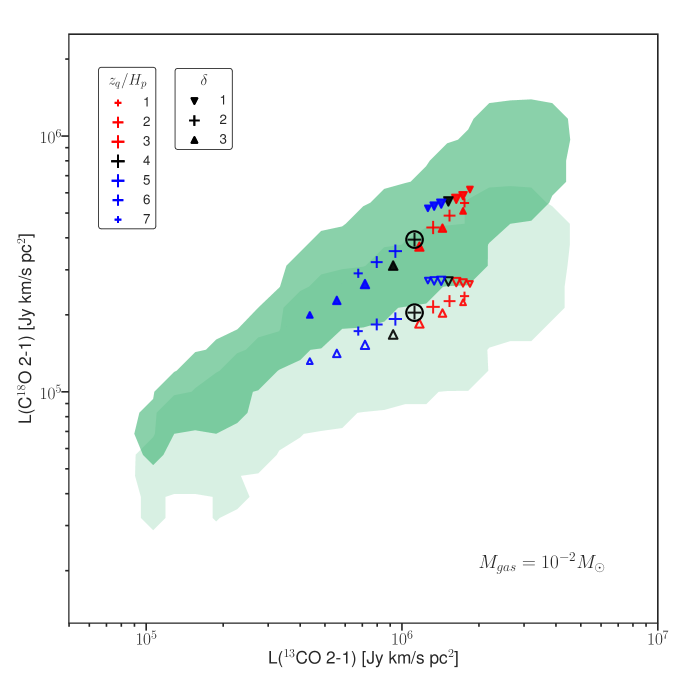
Figure 11.— The effect of different vertical temperature profiles on the ¹³CO and C¹⁸O 2–1 line luminosities. The green shaded areas outline the regions within which 99% of the full model grid points lie for disks with $M_{\rm gas}=0.01\,M_{\odot}$. The lighter green area represents the models with selective photodissociation, [CO]/[C¹⁸O]=1650. The different symbols, colors, and sizes indicate the vertical temperature profile parameters, $\delta$ and $z_{q}/H_{p}$, as shown in the legends at top left. The two fiducial values in the full grid, $\delta=2,z_{q}/H_{p}=4$, are circled. The variations in the line luminosities due to changes in the vertical temperature distribution are smaller than variations due to the range of disk parameters in Table 2.

References

- Aikawa et al. (1997) Aikawa, Y., Umebayashi, T., Nakano, T., & Miyama, S. M. 1997, ApJ, 486, L51
- Aikawa et al. (2002) Aikawa, Y., van Zadelhoff, G. J., van Dishoeck, E. F., & Herbst, E. 2002, A&A, 386, 622
- Alexander et al. (2013) Alexander, R., Pascucci, I., Andrews, S., Armitage, P., & Cieza, L. 2013, ArXiv e-prints
- Allègre et al. (2001) Allègre, C., Manhès, G., & Lewin, É. 2001, Earth and Planetary Science Letters, 185, 49
- Andrews et al. (2013) Andrews, S. M., Rosenfeld, K. A., Kraus, A. L., & Wilner, D. J. 2013, ApJ, 771, 129
- Andrews & Williams (2005) Andrews, S. M., & Williams, J. P. 2005, ApJ, 631, 1134
- Andrews & Williams (2007) —. 2007, ApJ, 671, 1800
- Andrews et al. (2011) Andrews, S. M., Wilner, D. J., Espaillat, C., Hughes, A. M., Dullemond, C. P., McClure, M. K., Qi, C., & Brown, J. M. 2011, ApJ, 732, 42
- Andrews et al. (2009) Andrews, S. M., Wilner, D. J., Hughes, A. M., Qi, C., & Dullemond, C. P. 2009, ApJ, 700, 1502
- Andrews et al. (2012) Andrews, S. M., et al. 2012, ApJ, 744, 162
- Astropy Collaboration et al. (2013) Astropy Collaboration et al. 2013, A&A, 558, A33
- Beckwith & Sargent (1991) Beckwith, S. V. W., & Sargent, A. I. 1991, ApJ, 381, 250
- Beckwith & Sargent (1993) —. 1993, ApJ, 402, 280
- Bergin et al. (2013) Bergin, E. A., et al. 2013, Nature, 493, 644
- Biller et al. (2013) Biller, B. A., et al. 2013, ApJ, 777, 160
- Bohlin et al. (1978) Bohlin, R. C., Savage, B. D., & Drake, J. F. 1978, ApJ, 224, 132
- Caselli et al. (1999) Caselli, P., Walmsley, C. M., Tafalla, M., Dore, L., & Myers, P. C. 1999, ApJ, 523, L165
- Chapillon et al. (2010) Chapillon, E., Parise, B., Guilloteau, S., Dutrey, A., & Wakelam, V. 2010, A&A, 520, A61
- D’Alessio et al. (2006) D’Alessio, P., Calvet, N., Hartmann, L., Franco-Hernández, R., & Servín, H. 2006, ApJ, 638, 314
- Dame et al. (2001) Dame, T. M., Hartmann, D., & Thaddeus, P. 2001, ApJ, 547, 792
- Dartois et al. (2003) Dartois, E., Dutrey, A., & Guilloteau, S. 2003, A&A, 399, 773
- Dent et al. (2005) Dent, W. R. F., Greaves, J. S., & Coulson, I. M. 2005, MNRAS, 359, 663
- Dullemond & Dominik (2005) Dullemond, C. P., & Dominik, C. 2005, A&A, 434, 971
- Dullemond et al. (2002) Dullemond, C. P., van Zadelhoff, G. J., & Natta, A. 2002, A&A, 389, 464
- Dutrey et al. (1996) Dutrey, A., Guilloteau, S., Duvert, G., Prato, L., Simon, M., Schuster, K., & Menard, F. 1996, A&A, 309, 493
- Dutrey et al. (1997) Dutrey, A., Guilloteau, S., & Guelin, M. 1997, A&A, 317, L55
- Dutrey et al. (1994) Dutrey, A., Guilloteau, S., & Simon, M. 1994, A&A, 286, 149
- Dutrey et al. (2003) —. 2003, A&A, 402, 1003
- Favre et al. (2013) Favre, C., Cleeves, L. I., Bergin, E. A., Qi, C., & Blake, G. A. 2013, ApJ, 776, L38
- Frerking et al. (1982) Frerking, M. A., Langer, W. D., & Wilson, R. W. 1982, ApJ, 262, 590
- Gammie (1996) Gammie, C. F. 1996, ApJ, 457, 355
- Goldsmith et al. (1997) Goldsmith, P. F., Bergin, E. A., & Lis, D. C. 1997, ApJ, 491, 615
- Gorti & Hollenbach (2008) Gorti, U., & Hollenbach, D. 2008, ApJ, 683, 287
- Güdel et al. (2007) Güdel, M., Padgett, D. L., & Dougados, C. 2007, Protostars and Planets V, 329
- Guilloteau et al. (2013) Guilloteau, S., Di Folco, E., Dutrey, A., Simon, M., Grosso, N., & Piétu, V. 2013, A&A, 549, A92
- Hartmann et al. (1998) Hartmann, L., Calvet, N., Gullbring, E., & D’Alessio, P. 1998, ApJ, 495, 385
- Howard (2013) Howard, A. W. 2013, Science, 340, 572
- Hughes et al. (2011) Hughes, A. M., Wilner, D. J., Andrews, S. M., Qi, C., & Hogerheijde, M. R. 2011, ApJ, 727, 85
- Hughes et al. (2007) Hughes, A. M., Wilner, D. J., Calvet, N., D’Alessio, P., Claussen, M. J., & Hogerheijde, M. R. 2007, ApJ, 664, 536
- Hughes et al. (2008) Hughes, A. M., Wilner, D. J., Qi, C., & Hogerheijde, M. R. 2008, ApJ, 678, 1119
- Jonkheid et al. (2007) Jonkheid, B., Dullemond, C. P., Hogerheijde, M. R., & van Dishoeck, E. F. 2007, A&A, 463, 203
- Jørgensen et al. (2002) Jørgensen, J. K., Schöier, F. L., & van Dishoeck, E. F. 2002, A&A, 389, 908
- Jura et al. (2012) Jura, M., Xu, S., Klein, B., Koester, D., & Zuckerman, B. 2012, ApJ, 750, 69
- Kamp & Dullemond (2004) Kamp, I., & Dullemond, C. P. 2004, ApJ, 615, 991
- Kamp et al. (2011) Kamp, I., Woitke, P., Pinte, C., Tilling, I., Thi, W.-F., Menard, F., Duchene, G., & Augereau, J.-C. 2011, A&A, 532, A85
- Kastner et al. (1997) Kastner, J. H., Zuckerman, B., Weintraub, D. A., & Forveille, T. 1997, Science, 277, 67
- Lefloch et al. (1998) Lefloch, B., Castets, A., Cernicharo, J., Langer, W. D., & Zylka, R. 1998, A&A, 334, 269
- Lesniak & Desch (2011) Lesniak, M. V., & Desch, S. J. 2011, ApJ, 740, 118
- Lynden-Bell & Pringle (1974) Lynden-Bell, D., & Pringle, J. E. 1974, MNRAS, 168, 603
- Mathews et al. (2013) Mathews, G. S., et al. 2013, A&A, 557, A132
- Menu et al. (2014) Menu, J., et al. 2014, A&A, 564, A93
- Nomura et al. (2007) Nomura, H., Aikawa, Y., Tsujimoto, M., Nakagawa, Y., & Millar, T. J. 2007, ApJ, 661, 334
- Panić et al. (2009) Panić, O., Hogerheijde, M. R., Wilner, D., & Qi, C. 2009, A&A, 501, 269
- Pavlyuchenkov et al. (2007) Pavlyuchenkov, Y., Semenov, D., Henning, T., Guilloteau, S., Piétu, V., Launhardt, R., & Dutrey, A. 2007, ApJ, 669, 1262
- Petigura & Marcy (2011) Petigura, E. A., & Marcy, G. W. 2011, ApJ, 735, 41
- Qi et al. (2011) Qi, C., D’Alessio, P., Öberg, K. I., Wilner, D. J., Hughes, A. M., Andrews, S. M., & Ayala, S. 2011, ApJ, 740, 84
- Qi et al. (2008) Qi, C., Wilner, D. J., Aikawa, Y., Blake, G. A., & Hogerheijde, M. R. 2008, ApJ, 681, 1396
- Qi et al. (2006) Qi, C., Wilner, D. J., Calvet, N., Bourke, T. L., Blake, G. A., Hogerheijde, M. R., Ho, P. T. P., & Bergin, E. 2006, ApJ, 636, L157
- Qi et al. (2013) Qi, C., et al. 2013, Science, 341, 630
- Ripple et al. (2013) Ripple, F., Heyer, M. H., Gutermuth, R., Snell, R. L., & Brunt, C. M. 2013, MNRAS, 431, 1296
- Roberge et al. (2006) Roberge, A., Feldman, P. D., Weinberger, A. J., Deleuil, M., & Bouret, J.-C. 2006, Nature, 441, 724
- Robitaille et al. (2006) Robitaille, T. P., Whitney, B. A., Indebetouw, R., Wood, K., & Denzmore, P. 2006, ApJS, 167, 256
- Rosenfeld et al. (2013a) Rosenfeld, K. A., Andrews, S. M., Hughes, A. M., Wilner, D. J., & Qi, C. 2013a, ApJ, 774, 16
- Rosenfeld et al. (2013b) Rosenfeld, K. A., Andrews, S. M., Wilner, D. J., Kastner, J. H., & McClure, M. K. 2013b, ApJ, 775, 136
- Rosenfeld et al. (2012) Rosenfeld, K. A., et al. 2012, ApJ, 757, 129
- Semenov & Wiebe (2011) Semenov, D., & Wiebe, D. 2011, ApJS, 196, 25
- Shimajiri et al. (2014) Shimajiri, Y., et al. 2014, A&A, 564, A68
- Sun et al. (2006) Sun, K., Kramer, C., Ossenkopf, V., Bensch, F., Stutzki, J., & Miller, M. 2006, A&A, 451, 539
- Tafalla et al. (2002) Tafalla, M., Myers, P. C., Caselli, P., Walmsley, C. M., & Comito, C. 2002, ApJ, 569, 815
- Thi et al. (2004) Thi, W.-F., van Zadelhoff, G.-J., & van Dishoeck, E. F. 2004, A&A, 425, 955
- Thi et al. (2010) Thi, W.-F., et al. 2010, A&A, 518, L125
- van der Marel et al. (2013) van der Marel, N., et al. 2013, Science, 340, 1199
- van Dishoeck & Black (1988) van Dishoeck, E. F., & Black, J. H. 1988, ApJ, 334, 771
- van Zadelhoff et al. (2001) van Zadelhoff, G.-J., van Dishoeck, E. F., Thi, W.-F., & Blake, G. A. 2001, A&A, 377, 566
- Visser et al. (2009) Visser, R., van Dishoeck, E. F., & Black, J. H. 2009, A&A, 503, 323
- Weidenschilling (1977) Weidenschilling, S. J. 1977, MNRAS, 180, 57
- Williams & Cieza (2011) Williams, J. P., & Cieza, L. A. 2011, ARA&A, 49, 67
- Wilson & Rood (1994) Wilson, T. L., & Rood, R. 1994, ARA&A, 32, 191
- Woitke et al. (2009) Woitke, P., Kamp, I., & Thi, W.-F. 2009, A&A, 501, 383
- Woitke et al. (2010) Woitke, P., Pinte, C., Tilling, I., Ménard, F., Kamp, I., Thi, W.-F., Duchêne, G., & Augereau, J.-C. 2010, MNRAS, 405, L26
- Zuckerman & Song (2004) Zuckerman, B., & Song, I. 2004, ARA&A, 42, 685