Improving Texture Categorization with Biologically Inspired Filtering

Abstract

Within the domain of texture classification, a lot of effort has been spent on local descriptors, leading to many powerful algorithms. However, preprocessing techniques have received much less attention despite their important potential for improving the overall classification performance. We address this question by proposing a novel, simple, yet very powerful biologically-inspired filtering (BF) which simulates the performance of human retina. In the proposed approach, given a texture image, after applying a DoG filter to detect the “edges”, we first split the filtered image into two “maps” alongside the sides of its edges. The feature extraction step is then carried out on the two “maps” instead of the input image. Our algorithm has several advantages such as simplicity, robustness to illumination and noise, and discriminative power. Experimental results on three large texture databases show that with an extremely low computational cost, the proposed method improves significantly the performance of many texture classification systems, notably in noisy environments. The source codes of the proposed algorithm can be downloaded from https://sites.google.com/site/nsonvu/code.

I Introduction

Texture classification is a fundamental issue in computer vision and image processing, playing a significant role in many applications such as medical image analysis, remote sensing, object recognition, document analysis, environment modeling, content-based image retrieval and many more. As the demand of such applications increases, texture classification has received considerable attention over the last decades and numerous novel methods have been proposed [1, 2, 3, 4, 5, 6, 7, 8, 9, 10, 11, 12, 13].

The texture classification problem is typically divided into the two subproblems of representation and classification [14], and to improve the overall quality of texture classification, researchers often focus on improving one of (or both) those steps. It is generally agreed that texture features play a very important role, and the last decade has seen numerous powerful descriptors being proposed such as modified SIFT (scale invariant feature transform) and intensity domain SPIN images [3], MR8 [5], the rotation invariant basic image features (BIF) [9], (sorted) random projections over small patches [15], local binary pattern (LBP) [2], and its variants [6, 7, 10, 11]. Also, different similarity measures such as $\chi^{2}$ statistic [2, 5], Bhattarcharyya distance [9], and Earth Mover’s Distance [3] are often used in conjunction with nearest neighbor classifiers [2], non-linear (kernel-based) support vector machines (SVMs) [16], or collaborative representation-based classifier [13]. Undoubtedly, an efficient preprocessing which enhances the robustness and discriminative power of texture features is an important factor towards enhancing such texture classification systems. However, to the best of our knowledge, there does not exist any “sufficiently efficient” preprocessing methods which can significantly improve texture features.

II Related work

Most of earlier work on texture analysis focused on the development of filter banks and on characterizing the statistical distributions of their responses, e.g., [1], until Ojala et al. [2] proposed LBP (Local Binary Patterns) and showed that statistics of small pixel neighborhoods are capable of achieving high discrimination. Since then, due to its impressive computational efficiency and good texture characterization, the dense LBP descriptor has gained considerable attention and has been intensively used in different applications such as face recognition [17].

LBPs are “micro” features capturing the distribution of the relationships between pixels in small-scale neighborhoods, but unfortunately, has several limitations such as small spatial support region, loss of local textural information, and rotation and noise sensitivities. To overcome those, a lot of effort has been done. To recover from the loss of information, local image contrast was introduced by Ojala et al. [2] as a complementary measure, and better performance has been reported. By a “completed” LBP model, Guo et al. [7] included both the magnitudes of local differences and the pixel intensity itself, and claimed better performance. In terms of locality, [6] proposed to extract global features from the Gabor filter responses as a complementary descriptor. Dominant LBP (DLBP) also presented in [6] rely on dominant patterns which were experimentally chosen from all rotation invariant patterns. Regarding noise robustness, Ojala et al. [2] introduced the concept of uniform and rotation invariant patterns (LBP^riu2), while Tan and Triggs [18] proposed local ternary patterns (LTP). Liu et al. [10] have recently generalized LBP with two different and complementary types of features which are extracted from local patches, based on pixel intensities and differences. Using this approach, the authors reported impressive texture classification rates. In [11], a “LBP like” feature, the Local Binary Count (LBC), is proposed, in which a pixel is encoded by the number of neighbors whose intensities are larger than that of the considered pixel. Heikkila et al. [19] exploit circular symmetric LBP (CS-LBP) for local interest region description. Also, presented in [20] are several LBP variants for image and video description, that is, the LBP histogram Fourier (LBP-HF) features, and the LBPs from three orthogonal planes (LBP-TOP) features. In [8], Chen et al. proposed WLD (Weber Local Descriptor) method based on the fact that human perception of a pattern depends not only on the change of a stimulus (such as sound, lighting) but also on the original intensity of the stimulus. WLD consists of two components: differential excitation and orientation.

An alternative method to improve the strength of texture descriptor is to perform efficient preprocessing. For example, in face recognition, Vu and Caplier [21, 22] applied the LBP operators upon three edge distribution maps across different directions, and reported state-of-the-art performance. However, to the best of our knowledge, with regard to feature extraction in texture classification, no such efficient preprocessing method exists (in [6], the DLBP features and Gabor filters are extracted separately). This is the motivation for the algorithm presented in this paper.

Neuroscience has made lots of progress in understanding the visual system and how images are transmitted to the brain. It is believed that the Difference of Gaussians (DoG) filter simulates how the human retina processes the images observed and extracts theirs details. We propose to somehow mimic the same strategy to generate richer and more robust information from the image before carrying out the feature extraction step.

The rest of the paper is structured as follows. Section  III details the proposed approach. Experimental results are presented in Section  IV and conclusions are finally drawn in Section  V.

III Proposed method

The main objective of the proposed method is to enhance robustness and discriminative power of texture classification systems at the level of preprocessing. To be invariant to rotation, one of crucial requirements in texture classification, techniques used should either discard all orientation information or capture relative orientation information. We follow the first idea and we use a simple yet efficient isotropic DoG filter which simulates the performance of human retina. Briefly speaking, given an input texture image, we first use a DoG filter to detect its “edges” and then split the filtered image into two “maps” alongside two sides of the detected edges (the term “edges” used here refer to the positions where there are changes in intensity). Feature extraction algorithms, e.g., the LBP encoding method, are then carried out on those resultant “maps” to obtain the final texture representation.

This section first briefly describes the human retina, in particular the bipolar cells by which our algorithm is inspired. We then detail the proposed method and discuss its properties.

III-A Model of Retinal Processing

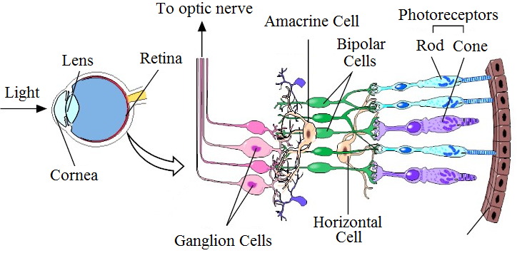
Figure 1: The retina lies at the back of the eye. Light passes through the ganglion, amacrine, bipolar, and horizontal cells and reaches the photoreceptors layers where it returns. Thus the signal is transmitted and processed within the retina in the inverse order, from the photoreceptors, horizontal and bipolar cells to amacrine and ganglion cells.

The retina lies at the back of the eye (see Fig. 1). Basically, it is made of three layers: the photoreceptors layer with cones and rods; the outer plexiform layer (OPL) with horizontal, bipolar and amacrine cells; and the inner plexiform layer (IPL) with ganglion cells. It is worth noting that the retina is capable to process both spatial and temporal signals but working on static images, we consider only the spatial processing in the retina.

Photoreceptors: rods and cones have quite different properties: rods have the ability to see at night, under conditions of very low illumination; cones have the ability to deal with bright signals. Photoreceptor layer plays therefore the role of a light adaptation filter.

Outer plexiform layer (OPL): the photoreceptor performs a low pass filter. Horizontal cells perform a second low pass filter. In OPL, bipolar cells calculate the difference between photoreceptor and horizontal cell responses. noise and low frequency illumination.

Typically, to model the processes of OPL, two Gaussian low pass filters with different standard deviations corresponding to the effects of photoreceptors and horizontal cells are used. Thus, bipolar cells act like a Difference of Gaussians (DoG) filter.

Inner plexiform layer (IPL): IPL works similarly to OPL but it performs on the temporal information rather than on the spatial one as in OPL.

In the literature, different algorithms inspired by the human retina have been proposed for different applications [23, 24, 25, 26]. In [23], Meylan et al. proposed a tone mapping algorithm using two nonlinear operators which approximates the photoreceptor. The two first layers of the retina, photoreceptor and OPL, have been modeled and successfully used for face recognition under difficult lighting conditions [24]. In [25], Benoit and Caplier modeled all the three layers for moving contours enhancement. Our algorithm is inspired by the performance of the bipolar cells.

III-B Details of the proposed method

In fact, there are two types of bipolar cells, called ON and OFF. The ON bipolar cells take into account the difference of photoreceptor and horizontal cell responses, whereas the OFF bipolar cells compute the difference of horizontal and photoreceptor cells. More precisely, if we apply a DoG filter on an image for simulating the bipolar cells, a “map” with positive and negative values will be obtained. Within this resultant “map”, the positive values and the absolute of the negatives values correspond respectively to the responses of the ON and OFF bipolar cells. The proposed algorithm is inspired by this “natural” performance of the human visual system in extracting image details, but also by the detailed analysis on the properties of the DoG filter itself.

The DoG filter is often used to approximate a LoG filter (Laplacian of Gaussian) due to its low computational cost. It calculates the second spatial derivative of an image. In areas where the image has a constant intensity, the filter response will be zero. Wherever an intensity change occurs, the filter will give a positive response on the darker side and a negative response on the lighter side. At a reasonably sharp edge between two regions of uniform but different intensities, the filter response will be:

• zero at a long distance from the edge

• positive on one side of the edge

• negative on the other side

• zero at some point in between, on the edge itself

Roughly speaking, the DoG filter can split the image details alongside two sides of the edge. Keeping in mind all these properties of the DoG filter, we propose a novel two-step preprocessing technique, as follows (Fig. 2):

Step 1: given an image $I_{in}$, it is first filtered by a band-pass Difference of Gaussians (DoG) filter which mimics the performance of bipolar cells:

$$I_{bf}=DoG*I_{in}$$ (1)

where the $DoG$ kernel is given by:

$$DoG=\frac{1}{2\pi\sigma_{1}^{2}}e^{-\frac{x^{2}+y^{2}}{2{\sigma}^{2}_{1}}}-\frac{1}{2\pi\sigma_{2}^{2}}e^{-\frac{x^{2}+y^{2}}{2{\sigma}^{2}_{2}}}$$ (2)

and where $\sigma_{1}$ and $\sigma_{2}$ correspond to the standard deviations of the low pass filters modeling photoreceptors and horizontal cells.

Step 2: the responses at bipolar cells are then decomposed into two “maps” corresponding to the image details alongside the two sides of the image edge (these decomposed “maps” also correspond to the responses on the ON and OFF cells):

$$I^{+}_{bf}(p)=\left\{\begin{array}[]{lll}I_{bf}(p)&if&I_{bf}(p)\geq\epsilon\\ 0&\lx@intercol\hfil otherwise\hfil\lx@intercol\end{array}\right.$$ (5)

$$I^{-}_{bf}(p)=\left\{\begin{array}[]{lll}|I_{bf}(p)|&if&I_{bf}(p)\leq-\epsilon\\ 0&\lx@intercol\hfil otherwise\hfil\lx@intercol\end{array}\right.$$ (8)

where the term $bf$ refers to “Biologically-inspired Filtering”, $p$ refers to a considered pixel, $\epsilon$ is slightly larger than zero to provide some stability in uniform regions: we do not take into account the uniform areas since these areas often contain noise rather than useful texture information.

Figure 2: Proposed processing chain: $I_{in},I_{bf},I^{+}_{bf},I^{-}_{bf}$ (left to right).

Then, in the feature extraction step, instead of the input image $I_{in}$, features are first extracted from the two images, $I^{-}_{bf}$ and $I^{+}_{bf}$, and then combined together. The resultant feature vector is considered as the descriptor of $I_{in}$. For example, with the conventional LBP method, the two histograms of LBP codes estimated from $I^{-}_{bf}$ and $I^{+}_{bf}$ are concatenated and considered as the texture representation of $I_{in}$.

Our algorithm is different from Local Ternary Patterns (LTP) [18] in several aspects. First, LTP splits the LBP codes into their positive and negative parts by comparing directly the pixel intensities, while we split the image filtered by DoG based on its edges. While LTP encodes the first order pixel-wise information, our method computes the second spatial derivative. Moreover, as a preprocessing technique, our algorithm can be easily combined with different feature extraction approaches, including LTP, to get more efficient methods. Also, we will show that the combination of the BF filter with the conventional LBP method considerably outperforms LTP.

III-C Properties

The proposed preprocessing has the following advantages:

• Robust to illumination and noise: the band-pass DoG filter removes both high frequency noise and low frequency illumination.

• Discriminative: with our technique, image details alongside two sides of the edges are obtained. We will experimentally show that features, which are extracted from these “maps” and combined together, convey richer information about object than features being extracted from an input image.

• Rotation insensitivity: our filter is isotropic and discards all orientation information, and is therefore independent to rotation.

• Low computational time: the proposed algorithm is extremely fast. With un-optimized Matlab code running on a laptop of CPU Intel Core i5 1.7Ghz (2G Ram), it takes only less than $0.9s$ to process 1000 images of 128$\times$128 pixels or $1.9s$ to process 1000 images of 200$\times$200 pixels.

IV Experimental Validation

IV-A Experimental Settings

IV-A1 Databases

The effectiveness of the proposed method is assessed by a series of experiments on three large and representative databases: Outex [27], CUReT (Columbia-Utrecht Reflection and Texture) [28], and UIUC [3].

The Outex database (examples are shown in Fig. 3) contains textural images captured from a wide variety of real materials. We consider the two commonly used test suites, Outex_TC_00010 (TC10) and Outex_TC_00012 (TC12), containing 24 classes of textures which were collected under three different illuminations (“horizon”, “inca”, and “t184”) and nine different rotation angles (0^∘, 5^∘, 10^∘, 15^∘, 30^∘, 45^∘, 60^∘, 75^∘ and 90^∘).

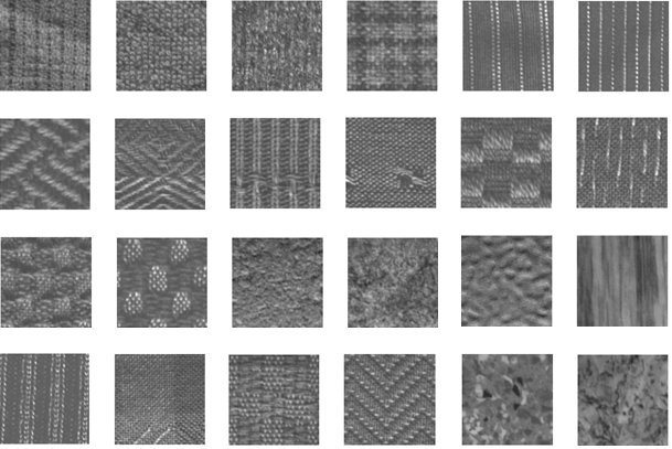
Figure 3: Texture images with the illumination condition “inca” and zero degree rotation angle from the 24 classes of textures on the Outex database.

The CUReT database (examples are shown in Fig. 4) contains 61 texture classes, each having 205 images acquired at different viewpoints and illumination orientations. There are 118 images shot from a viewing angle of less than 60^∘. From these 118 images, as in [5, 7], we selected 92 images, from which a sufficiently large region could be cropped (200$\times$200) across all texture classes. All the cropped regions are converted to grey scale.

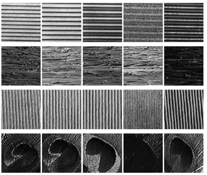
Figure 4: Examples of texture images from the CUReT database.

The UIUC texture database includes 25 classes with 40 images in each class. The resolution of each image is 640$\times$480. The database contains materials imaged under significant viewpoint variations (examples are shown in Fig. 5).

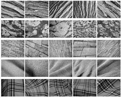
Figure 5: Examples of texture images on the UIUC database.

IV-A2 Feature Extraction

To validate the proposed preprocessing algorithm, we evaluate how far it can improve the performance of texture classification systems based on several popular features, including SIFT, LBP-based descriptors, WLD (Weber Local Descriptor) [8], and LBC (Local Binary Count - a recent LBP variant) [11]. Note that, the combination of BF with other more powerful features such as the extended LBP method [10] is beyond the scope of this paper and will be considered in future work.

Concerning LBP, we use the completed model proposed in [7], which gathers three individual operators: CLBP-Sign (CLBP_S) which is equivalent to the conventional LBP, CLBP-Magnitude (CLBP_M) which measures the local variance of magnitude, and CLBP-Center (CLBP_C) which extracts the local central information. Similarly, the completed LBC model with three different individual operators is considered. When using LBP and LBC features, only rotation invariant uniform patterns are considered .

We also apply the combination strategies presented in [7]. There are two ways to combine the CLBP_S and CLBP_M codes: by concatenation or jointly. In the first way, the histograms of the CLBP_S and CLBP_M codes are computed separately, and then concatenated together. This CLBP scheme is referred to as “CLBP_S_M”. In the second way, a joint 2D histogram of the CLBP_S and CLBP_M codes is calculated and denoted as “CLBP_S/M”.

The three operators, CLBP_S, CLBP_M and CLBP_C (resp. CLBC_S, CLBC_M and CLBC_C in the completed LBC model), can be combined in two ways, jointly or hybridly. In the first way, a 3D joint histogram of them is built and denoted by “CLBP_S/M/C”. In the second way, a 2D joint histogram, “CLBP_S/C” or “CLBP_M/C” is built first, and then is converted to a 1D histogram, which is then concatenated with CLBP_M or CLBP_S to generate a joint histogram, denoted by “CLBP_M_S/C” or “CLBP_S_M/C”.

The WLD method [8] consists of two components: differential excitation and orientation. The differential excitation component is a function of the ratio between two terms: one is the relative intensity differences of a current pixel against its neighbors; the other is the intensity of the current pixel. The orientation component is the gradient orientation of the current pixel. For a given image, the two components are used to construct a concatenated WLD histogram.

We therefore apply these schemes on the original texture images and on the preprocessed images, obtained as presented in Section III.

When using SIFT (in this paper, we used the original SIFT introduced by Lowe [29]), given an image, co-variant regions (patches around keypoints) are first detected and then processed by the BF filter to generate richer information. Finally, SIFT descriptors are computed from “generated patches” and used to represent corresponding co-variant regions in the original image. In other words, feature keypoints are detected in original image while feature descriptors are computed in images filtered by the BF approach.

IV-A3 Similarity Measure and Classifier

Classification rates are reported using the simple nearest neighbor classifier.

For all CLBP, CLBC and WLD descriptors, the $\chi^{2}$ distance is used to measure the similarity between two texture images. If $H=\{h_{i}\}$ and $K=\{k_{i}\},(i=1,2,...,n)$ denote two histograms corresponding to the representations of two images, the $\chi^{2}$ distance is calculated as: $\chi^{2}(H,K)=\sum_{i=1}^{n}\frac{(h_{i}-k_{i})^{2}}{h_{i}+k_{i}}$.

Concerning SIFT, keypoints from two images are compared and matched using the L2 norm of the difference between their descriptors as measure. The final similarity score between two considered images is the average value of distance between their matched keypoints (when there are any matched keypoints between two images, the score is set very high).

IV-B Parameter Exploration

In this section, we study how the parameters of the BF filter influence final performance. Parameters to be chosen include the two standard deviations $\sigma_{1}$ and $\sigma_{2}$ defining the low and high cutoff frequencies of the band pass $DoG$ filter, and the threshold $\epsilon$. A critical constraint is $\sigma_{1}<\sigma_{2}$ (recall that these correspond respectively to the parameters of the blurring filters being performed in photoreceptors and horizontal cells).

The experiments described in this section were conducted on the Outex database. We compute the average classification rates on the three test suites (TC10, TC12t and TC12h) with different parameters of the BF filter. For each texture descriptor or combination strategy in the completed LBP/LBC model used (each descriptor was also tested with different parameters itself), 150 BF filters with different parameters were evaluated:

• $\sigma_{1}\in\{0.5,0.75,1,1.25,1.5\}$

• $\sigma_{2}\in\{2,3,4,5,6\}$

• $\epsilon\in\{0.05,0.1,0.15,0.2,0.25,0.3\}$

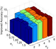
(a) CLBC_S_R=2

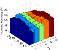
(b) CLBC_M_R=2

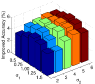
(c) CLBC_S/M_R=2

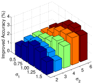
(d) CLBC_S/M/C_R=2

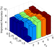
(e) CLBP_S/C_R=1

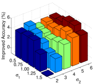
(f) CLBP_M/C_R=2

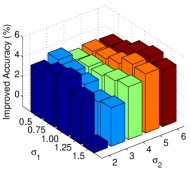
(g) CLBP_S_M/C_R=2

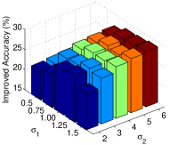
(h) WLD

Figure 6: Improved classification accuracy obtained with different standard deviations ($\sigma_{1}$ and $\sigma_{2}$) of the BF filter. These rates are calculated by averaging classification rates with different $\epsilon$ on the three test suites (TC_10, TC_12 “t”, TC_12 “h”) of the Outex database.

IV-B1 Determining $\sigma_{1}$ and $\sigma_{2}$

For each pair of $\sigma_{1}$ and $\sigma_{2}$, the average classification rates are calculated for varying $\epsilon$. Fig.  6 shows the improved classification rates obtained when the proposed BF filter is used with different descriptors and combination strategies (due to space limitations, the most informative results are depicted). In a few cases when the values of $\sigma_{1}$ and $\sigma_{2}$ are very close (see Fig.  6 (f) and (g) with $\sigma_{1}=1.5,\sigma_{2}=2,$), the BF filtering leads to slight improvements. This can be explained by the fact that when $\sigma_{1}$ is slightly smaller than $\sigma_{2}$, a high amount of image information is ignored. More precisely, in such cases, the information at numerous frequencies (low and high) is removed. In all the other cases, our BF filters always result an in important gain of classification accuracy for all evaluated descriptors (further details will be discussed in Section IV.D). When using CLBC_S/M/C, CLBP_S/M/C or WLD (Fig.  6 (d) and (h)), the performance of the BF filter with $\sigma_{1}=0.5$ is slightly worse than the others. Therefore, in general, we propose to use $\sigma_{1}\in\{0.7,1.3\}$ and $\sigma_{2}\in\{3,6\}$. Indeed, in our tests, we obtained the best results with $\sigma_{1}=1.25$ and $\sigma_{2}=5,6$ (refer to Section IV.D).

IV-B2 Determining $\epsilon$

Recall that the threshold $\epsilon$ being slightly larger than zero is used to provide some stability in uniform regions (the uniform areas containing noise rather than useful texture information are not taken into account). To determine $\epsilon$, we compute the average of classification rates across different $\epsilon$: for each value of $\epsilon$, we use 12 pairs of ($\sigma_{1},\sigma_{2}$), $\sigma_{1}=0.75,1.00,1.25$ and $\sigma_{2}=3,4,5,6$. As can be seen from Fig. 7, the performance of the BF filter with $\epsilon=0.05,0.1,0.15$ is similar (the BF filter with $\epsilon=0.15$ performs slightly better the others) while it begins to drop when $\epsilon\geq 0.2$. This can be explained by the fact that when the value of $\epsilon$ is too high, useful information is lost.

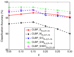
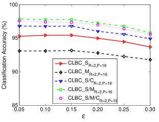
Figure 7: Classification rates for different descriptors with different values of the threshold $\epsilon$. These rates are calculated by averaging classification rates on the three test suites (TC_10, TC_12 “t”, TC_12 “h”) of the Outex database with different values of $\sigma_{1}$ and $\sigma_{2}$.

In conclusion, the BF filtering performs well with different parameters: $\sigma_{1}\in[0.7,1.3]$ and $\sigma_{2}\in[3,6]$, $\epsilon\in[0.05,0.15]$. We obtained the best results with $\sigma_{1}=1.25$, $\sigma_{2}=5,6$, and $\epsilon=0.15$ (when CLBP and CLBC are used). However, with the main goal of showing that our preprocessing technique is very efficient in general, in the rest of this paper, without exception, we will report the results with the default parameters: $\sigma_{1}=1$, $\sigma_{2}=4$, and $\epsilon=0.1$.

IV-C Comparison with other Preprocessing Algorithms

In order to show the advantage of our algorithm, this section compares its performance with other preprocessing techniques. It would be worth noting that in the literature, to improve the overall quality of texture classification, researchers often focus on improving one of (or both) the two steps of representation and classification, and to the best of our knowledge, there does not exist any work considering properly preprocessing techniques. We propose to compare here the BF filter with several existing preprocessing techniques: (1) “traditional” gamma correction method (it is shown in [6] that histogram equalization (HE) degrades in general the performance of texture descriptor, thus we do not compare HE and BF here); (2) the typical DoG filter without dividing the filtered image into two parts as our BF method; and (3) Gaussian derivative filters (zeroth-order, first order and second order derivative filters). For all sorts of considered filters, we compute the classification rates with different parameters (e.g., different scales for Gaussian filters) and use their best classification rates to compare with our “mean” results (we do not use the optimal parameters).

We also decomposed the image filtered by Gaussian first derivative filter (gradient magnitude map) regarding the pixel gradient orientation and then extract the features on those decomposed images. However, contrary to face recognition [30, 31], this idea does not work for texture classification. This is due to the fact that considered texture images contain rotation transforms and dividing them across “absolute” orientations leads to sensitivity to rotation. More precisely, Gaussian first derivative filter is defined as:

$$DtG(x,y,\sigma)=\sqrt{(G_{x}(x,y,\sigma))^{2}+(G_{y}(x,y,\sigma))}$$ (9)

where $G_{x}(x,y,\sigma)=\frac{dG(x,y,\sigma)}{dx}=-\frac{x}{2\sigma^{3}\pi}e^{-\frac{x^{2}+y^{2}}{2\sigma^{2}}}$ and $G_{y}(x,y,\sigma)=\frac{dG(x,y,\sigma)}{dy}=-\frac{y}{2\sigma^{3}\pi}e^{-\frac{x^{2}+y^{2}}{2\sigma^{2}}}$.

Using Gabor filters as preprocessing (the global mean of the responses of Gabor filters) was also considered but in our experiments, they perform worse than Gaussian derivative filters. The classification results of different preprocessing techniques are shown in Fig. 8 (only the most informative results are depicted). As can be seen, preprocessing techniques can enhance the performance of texture classification, and in all cases, our BF filter always performs the best, showing the advantage of the proposed preprocessing approach.

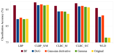
(a) Outex_TC_00010

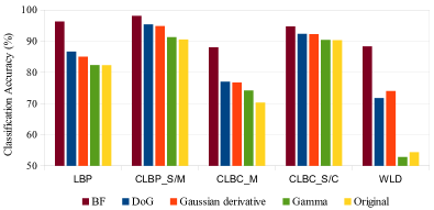
(b) Outex_TC_00012 (t184)

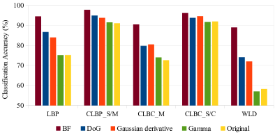
(c) Outex_TC_00012 (horizon)

Figure 8: Comparison of different preprocessing techniques.

IV-D Results on the Outex Database

This section presents and discusses in more detail the results obtained on the Outex database. We first show how far our preprocessing algorithm can improve the texture descriptors “in general”: the default parameters ($\sigma_{1}=1$, $\sigma_{2}=4$, and $\epsilon=0.1$) are used. Then, with the optimal parameters, we show that combining our preprocessing approach with known texture descriptors can outperform various state-of-the-art texture classification systems. The results obtained when combining BF with CLBP will be analyzed in detail while other results will de discussed more quickly.

IV-D1 Improving the performance of the completed LBP model

For each method considered, three classification rates are computed with different parameters: $P$ being the total number of involved neighbors per pixel and $R$ the radius of the neighborhood.

TABLE I: CLASSIFICATION RATES OBTAINED ON THE OUTEX DATABASE WHEN USING CLBP AS DESCRIPTOR.

	$R=1,P=8$				$R=2,P=16$				$R=3,P=24$
	TC10	TC12		Average	TC10	TC12		Average	TC10	TC12		Average
		t184	horizon			t184	horizon			t184	horizon
LTP	94.14	75.88	73.96	81.33	96.95	90.16	86.94	91.35	98.20	93.59	89.42	93.74
CLBP_S	84.81	65.46	63.68	71.31	89.40	82.26	75.20	82.28	95.07	85.04	80.78	86.96
BF + CLBP_S	96.17	92.92	92.75	93.95	97.73	96.29	94.58	96.20	99.11	96.62	93.15	96.29
Gain	+11.36	+27.46	+29.07	+22.64	+8.33	+14.03	+19.38	+13.92	+4.04	+11.58	+12.37	+9.33
CLBP_M	81.74	59.30	62.77	67.93	93.67	73.79	72.40	79.95	95.52	81.18	78.65	85.11
BF + CLBP_M	91.43	79.40	83.59	84.81	97.29	89.47	93.59	93.45	97.08	92.78	94.28	94.71
Gain	+9.69	+20.10	+20.82	+16.08	+3.62	+15.68	+21.19	+13.50	+1.56	+11.60	+15.63	+9.60
CLBP_M/C	90.36	72.38	76.66	79.80	97.44	86.94	90.97	91.78	98.02	90.74	90.69	93.15
BF + CLBP_M/C	94.43	83.84	86.53	88.27	99.24	91.34	94.65	95.08	98.93	95.53	96.46	96.97
Gain	+4.07	+11.46	+9.87	+8.47	+1.80	+4.40	+3.68	+3.30	+0.91	+4.79	+5.77	+3.82
CLBP_S_M/C	94.53	81.87	82.52	86.30	98.02	90.99	91.08	93.36	98.33	94.05	92.40	94.92
BF + CLBP_S_M/C	96.69	90.76	91.48	92.98	99.45	95.56	96.16	97.06	99.32	96.83	96.50	97.55
Gain	+2.16	+8.89	+8.96	+6.68	+1.43	+4.57	+5.08	+3.70	+0.99	+2.78	+4.10	+2.63
CLBP_S/M	94.66	82.75	83.14	86.85	97.89	90.55	91.11	93.18	99.32	93.58	93.35	95.41
BF + CLBP_S/M	97.06	94.84	93.49	95.13	99.35	98.06	97.80	98.40	99.61	97.62	97.57	98.26
Gain	+2.40	+12.09	+10.35	+8.28	+1.46	+7.51	+6.69	+5.22	+0.29	+4.04	+4.22	+2.85
CLBP_S/M/C	96.56	90.30	92.29	93.05	98.72	93.54	93.91	95.39	98.93	95.32	94.53	96.26
BF + CLBP_S/M/C	97.40	95.28	94.58	95.51	99.50	96.87	96.62	97.67	99.63	97.52	97.71	98.29
Gain	+0.84	+4.98	+2.29	+2.46	+0.78	+3.33	+2.71	+2.28	+0.70	+2.20	+3.18	+2.03

Table I reports the experimental results of different methods, from which we can get some interesting findings:

• For all considered features or combination strategies with their different parameter settings, using our algorithm as preprocessing results in important gains in performance. For example, when combining our BF filtering with the conventional LBP (CLBP_S in Table I), with the three parameter configurations, the average improvements are respectively 22.64$\%$, 13.92$\%$, and 9.33$\%$. Similarly, when combining the BF filtering with CLBP_M, the average improvements with the three parameters are respectively 16.08$\%$, 13.50$\%$, and 9.60$\%$.

• With the same parameters, the simple combination “BF $+$ LBP” outperforms all “original” combination schemes which must gather the information of sign, magnitude, and/or center (by term “original”, we refer to algorithms which do not use our filtering as preprocessing). For example, with ($R=1,P=8$), the classification rate of “BF $+$ LBP” is 93.95% while the results of CLBP_S/M and CLBP_S/M/C are respectively 86.85% and 93.05%. Similarly, with ($R=2,P=16$), the classification rate of “BF $+$ LBP” is 96.20% while the results of CLBP_S/M and CLBP_S/M/C are respectively 93.18% and 95.39%.

• ‘BF $+$ LBP” clearly outperforms LTP with all considered parameters on all test suites.

• To compare the complexities of these algorithms, three factors must be considered: preprocessing time, feature extraction time and feature size which affects the classification time. As can be seen in Table II, our preprocessing step requires only $0.87ms$ (resp. $1.91ms$) to process an image of 128$\times$128 (resp. 200$\times$200) pixels, this additional time being really small. When using the BF filter, the feature extraction time and feature size are doubled, but there are important gains in classification rates. The feature extraction time of “BF $+$ LBP” is similar to that of CLBP_S_M/C and CLBP_S/M (see Table II). However, while the feature sizes of CLBP_S_M/C are 30, 54, and 78, the feature sizes of CLBP_S/M are 100, 324, and 676 for ($R=1,P=8$), ($R=2,P=16$), and ($R=3,P=24$), respectively, the feature sizes of “BF $+$ LBP” are much smaller: they are 20, 36, and 52 for ($R=1,P=8$), ($R=2,P=16$), and ($R=3,P=24$) respectively.

• “BF + CLBP_S” outperforms the best “original” scheme, the CLBP_S/M/C method. For instance, with (R=2, P=16), the classification rates of “BF + CLBP_S” and CLBP_S/M/C are 96.20% and 95.39% respectively. However, the feature dimensions of “BF + CLBP_S” are considerably smaller than those of CLBP_S/M/C. With the three parameter settings, the feature dimensions of “BF + CLBP_S” are respectively 20, 36 and 52, while those of CLBP_S/M/C are respectively 200, 648 and 1352. Thus, our classification step is faster, notably when texture classification is performed on large databases. In such systems, once a vector feature is extracted from the test image, it is compared and matched against (up to) thousands of other feature vectors corresponding to training samples in the database.

TABLE II: COMPARISON OF THE COMPLEXITY OF DIFFERENT TEXTURE REPRESENTATIONS.

Method	FET1	FET2	Feat. Size	MT
BF	0.87	1.91	-	-
LBPP=16	4.33	12.21	18	0.79
BF + LBPP=16	9.92	25.96	36	1.58
CLBP_S_M/CP=16	11.22	27.67	54	2.30
CLBP_S/MP=16	10.23	25.97	324	17.48
LBPP=24	7.01	17.21	26	1.11
BF + LBPP=24	14.95	36.69	52	2.21
CLBP_S_M/CP=24	15.31	39.17	78	4.25
CLBP_S/MP=24	14.98	37.13	676	45.63

Time is expressed in milliseconds. With experiments on 1000 images, the average time per image is computed. FET: Feature Extraction Time. FET₁ and FET₂ are feature extraction time on images of $128\times 128$ and $200\times 200$ pixels, respectively. MT: Matching Time, this corresponds to the time required for comparing the descriptor of the test image with those of reference images (we consider here a reference set of 2000 samples).

IV-D2 Improving the performance of the CLBC, WLD, and SIFT methods

TABLE III: CLASSIFICATION RATES OBTAINED ON THE OUTEX DATABASE WHEN USING CLBC AND WLD AS DESCRIPTOR.

	$R=1,P=8$				$R=2,P=16$				$R=3,P=24$
	TC10	TC12		Average	TC10	TC12		Average	TC10	TC12		Average
		t184	horizon			t184	horizon			t184	horizon
CLBC_S	82.94	65.02	63.17	70.38	88.67	82.57	77.41	82.88	91.35	83.82	82.75	85.97
BF + CLBC_S	96.30	92.55	92.96	93.94	98.41	95.28	95.32	96.34	98.96	95.35	94.44	96.25
Gain	+13.36	+27.53	+29.79	+23.56	+9.74	+12.71	+17.91	+13.46	+7.61	+11.53	+11.69	+10.28
CLBC_M	78.96	53.63	58.01	63.53	92.45	70.35	72.64	78.48	91.85	72.59	74.58	79.67
BF + CLBC_M	90.31	79.91	83.56	84.59	97.94	87.94	90.46	92.11	96.82	88.73	91.55	92.37
Gain	+11.35	+26.28	+25.55	+21.06	+5.49	+17.59	+17.82	+13.63	+4.97	+16.14	+16.97	+12.70
CLBC_S/M	95.23	82.13	83.59	86.98	98.10	89.95	90.42	92.82	98.70	91.41	90.25	93.45
BF + CLBC_S/M	96.74	94.72	92.78	94.75	99.48	97.89	97.31	98.23	99.40	97.57	97.92	98.30
Gain	+1.51	+12.59	+9.19	+7.77	+1.38	+7.94	+6.89	+5.41	+0.70	+6.16	+7.67	+4.85
CLBC_S/M/C	97.16	89.79	92.92	93.29	98.54	93.26	94.07	95.29	98.78	94.00	93.24	95.67
BF + CLBC_S/M/C	97.40	95.09	94.12	95.54	99.51	96.41	95.83	97.25	99.32	97.78	97.85	98.32
Gain	+0.24	+5.30	+1.20	+2.25	+0.97	+3.15	+1.76	+1.96	+0.54	+3.78	+4.61	+2.65
CLBC_CLBP [11]	96.88	90.25	92.92	93.35	98.83	93.59	94.26	95.56	98.96	95.37	94.72	96.35

	TC10	TC12		Average
		t184	horizon
WLD	77.86	58.26	54.42	63.51
BF + WLD	95.70	88.33	89.03	91.02
Gain	+17.84	+30.07	+34.61	+26.51
SIFT	83.78	74.10	75.58	77.82
BF + SIFT	94.77	87.78	88.94	90.50
Gain	+10.99	+13.68	+13.66	+12.78

This section considers the performance of the BF filter when combining with the CLBC, WLD and SIFT descriptors. The experimental results of different methods are reported in Table III, from which we can get similar interesting findings as in the experiments with the completed LBP model:

• For all considered features or combination strategies with their different parameter settings, using the BF filter as preprocessing results in important gains in performance. For example, when combining our BF filtering with the conventional LBC, with the three parameter configurations, the average improvements are respectively 23.56%, 13.46%, and 10.28%. Similarly, when combining the BF filtering with CLBC_M, the average improvements with the three parameters are respectively 21.06%, 13.63%, and 12.70%. When combining the BF filter with WLD and SIFT, we obtained important improvements of 26.51% and 12.78% respectively.

• With the same parameters, the simple combination “BF $+$ LBC” outperforms all “original” combination schemes.

• Also, both the simple combinations “BF + LBP” and “BF + LBC” are comparable (with $R=3$) or even outperform “CLBC_CLBP” [11] (CLBP_S/M/C + CLBC_S/M/C) which combines two completed models of features, the completed LBP and the completed LBC, and use six operators (three for each model).

IV-D3 Further Experiments and Discussions

We compare now our results obtained with the optimal parameters of the BF filter to different state-of-the-art results. From Fig. 9, we can see that:

• Our simple ‘BF $+$ LBP” already outperforms many state-of-the-art algorithms, including NGF, DLBP [6], and VZ_MR8, VZ_Joint [5]. The method of Liao et al. in [6] has to combine the Normalized Gabor Filter (NGF) and a more complicated LBP variant, DLBP, but its results are still inferior to ours.

• Our combination BF + CLBP_S/M and BF + CLBC_S/M outperform all the considered algorithms, even the best results of the multi-scale NI/RD/CI (Neighboring Intensities, Radial Difference, and Central Intensity) [10] which are respectively 99.7$\%$, 98.7$\%$, and 98.1$\%$ for the three test suites of the Outex database. To the best of our knowledge, our classification rates obtained are the best ever results on this database.

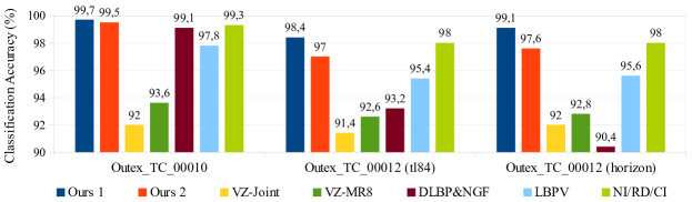
Figure 9: Comparison of the best classification scores. Ours 1: BF + CLBP_S/M $(R=2,P=16)$, Ours 2: simple BF + LBP $(R=2,P=16)$. Also, with these optimal parameters, our BF + CLBC_S/M $(R=2)$ obtains the very high classification rates on these three test suites which are respectively 99.53$\%$, 98.54$\%$, and 98.89$\%$. For a fair comparison, the best results of single scale NI/RD/CI $(R=2)$ [10] are considered in this figure.

IV-E Results on the CUReT database

In the experiments on the CUReT database , as in [3, 7], to get statistically significant experimental results, $N$ training images were randomly chosen from each class while the remaining $92-N$ images per class were used as the test set (note that, we return to the default parameters of the BF filter).

The average classification rates (with different parameters of CLBP) over a hundred random splits are reported in Table IV, from which we can get similar interesting observations as in the experiments on the Outex database:

TABLE IV: CLASSIFICATION RATES OBTAINED ON THE CURET DATABASE.

	$R=1,P=8$				$R=3,P=16$				$R=5,P=24$
N	46	23	12	6	46	23	12	6	46	23	12	6
CLBP_S	80.63	74.81	67.84	58.70	86.37	81.05	74.62	66.17	86.37	81.21	74.71	66.55
BF + CLBP_S	91.97	86.43	81.08	72.17	93.16	88.13	81.94	74.45	89.19	86.22	77.91	69.67
Gain	+11.34	+11.62	+13.24	+13.47	+6.79	+7.08	+7.32	+8.28	+2.82	+5.01	+3.20	+3.12
CLBP_M	75.20	67.96	60.27	51.49	85.48	79.01	71.24	61.59	82.16	76.23	69.22	60.45
BF + CLBP_M	91.53	85.81	78.04	70.18	92.78	89.43	82.74	74.82	92.43	87.57	81.65	74.01
Gain	+16.33	+17.85	+17.77	+18.69	+7.30	+10.42	+11.50	+13.23	+10.27	+11.34	+12.43	+13.56
CLBP_M/C	83.26	75.58	66.91	56.45	91.42	85.73	78.05	68.14	89.48	83.54	75.96	66.41
BF + CLBP_M/C	94.63	90.84	83.87	76.45	95.64	92.40	85.67	78.76	94.50	89.67	83.98	76.68
Gain	+11.37	+15.26	+16.96	+20.00	+4.22	+6.67	+7.62	+10.62	+5.02	+6.13	+8.02	+10.27
CLBP_S_M/C	90.34	84.52	76.42	66.31	93.87	89.05	82.46	72.51	93.22	88.37	81.44	72.01
BF + CLBP_S_M/C	95.68	91.77	86.77	78.97	96.08	92.46	85.28	80.84	95.01	91.99	84.52	77.67
Gain	+5.34	+7.25	+10.35	+12.66	+2.21	+3.41	+2.82	+8.33	+1.79	+3.62	+3.08	+5.66
CLBP_S/M	93.52	88.67	81.95	72.30	94.45	90.40	84.17	75.39	93.63	89.14	82.47	73.26
BF + CLBP_S/M	96.76	93.85	88.02	82.97	97.65	94.91	89.13	82.79	97.21	92.49	88.37	81.68
Gain	+3.24	+5.18	+6.07	+10.67	+3.20	+4.51	+4.96	+7.40	+3.58	+3.35	+5.90	+8.42
CLBP_S/M/C	95.59	91.35	84.92	74.80	95.86	92.13	86.15	77.04	94.74	90.33	83.82	74.46
BF + CLBP_S/M/C	97.20	93.89	89.26	82.75	97.04	94.25	88.57	82.02	95.82	91.69	86.97	79.24
Gain	+1.61	+2.54	+4.34	+7.95	+1.18	+2.12	+2.42	+4.98	+1.08	+1.36	+3.15	+4.78
VZ_MR8	97.79 (46), 95.03 (23), 90.48 (12), 82.90 (6)
VZ_Joint	97.66 (46), 94.58 (23), 89.40 (12), 81.06 (6)
Multiscale NI/RD/CI	97.29 (46)

• For all considered methods with different parameters, using our algorithm as preprocessing results in important gains in performance. For example, when combining BF with CLBP_M, with (R=1, P=8), the improvements with four different numbers of training images used ($N=46,23,12,6$) are respectively 16.33$\%$, 17.85$\%$, 17.77$\%$, and 18.69$\%$.

• In the CUReT database, there are scale and affine variations. While VZ_MR8 and VZ_Joint were designed with scale and affine invariance property, the CLBP operators we used have limited capability to address scale and affine invariance. However, interestingly, “BF + CLBP_S/M/C” still performs as well as VZ_MR8 and VZ_Joint. It also outperforms the recent multi-scale NI/RD/CI method [10] which must combine three descriptors at three scales.

IV-F Results on the UIUC database

TABLE V: CLASSIFICATION RATES OBTAINED ON THE UIUC DATABASE.

		20	15	10	5
R=1, P=8	CLBP_S	54.78	51.85	46.79	40.53
	BF + CLBP_S	87.79	77.24	75.82	69.13
	Gain	+33.01	+25.39	+29.03	+28.60
	CLBP_M	57.52	54.14	50.11	40.95
	BF + CLBP_M	83.63	75.26	72.04	63.11
	Gain	+26.11	+21.12	+21.93	+22.16
	CLBP_S/M	81.80	78.55	74.8	64.84
	BF + CLBP_S/M	91.21	87.15	83.19	75.65
	Gain	+9.41	+8.60	+8.39	+10.81
	CLBP_S/M/C	87.64	85.70	82.65	75.05
	BF + CLBP_S/M/C	91.47	87.41	83.96	76.24
	Gain	+3.83	+1.71	+1.31	+1.19
R=2, P=16	CLBP_S	61.04	55.84	51.77	41.88
	BF + CLBP_S	90.76	88.13	85.07	76.22
	Gain	+29.72	+32.29	+33.30	+34.34
	CLBP_M	72.12	68.99	64.47	57.06
	BF + CLBP_M	87.98	84.37	81.76	70.95
	Gain	+15.86	+15.38	+17.29	+13.89
	CLBP_S/M	87.87	85.07	80.59	71.64
	BF + CLBP_S/M	94.25	91.77	89.68	80.86
	Gain	+6.38	+6.70	+9.09	+9.22
	CLBP_S/M/C	91.04	89.42	86.29	78.57
	BF + CLBP_S/M/C	93.45	90.99	87.97	80.19
	Gain	+2.41	+1.57	+1.68	+1.62
R=3, P=16	CLBP_S	64.11	60.11	54.67	44.45
	BF + CLBP_S	91.24	87.46	82.87	73.12
	Gain	+27.13	+27.35	+28.20	+28.67
	CLBP_M	74.45	71.47	65.21	56.72
	BF + CLBP_M	89.78	86.01	81.07	71.12
	Gain	+15.33	+14.54	+15.86	+14.44
	CLBP_S/M	89.18	87.42	81.95	72.53
	BF + CLBP_S/M	94.14	91.99	89.61	80.98
	Gain	+4.96	+4.57	+7.66	+8.45
	CLBP_S/M/C	91.19	89.21	85.95	78.05
	BF + CLBP_S/M/C	93.78	91.64	88.12	80.23
	Gain	+2.59	+2.43	+2.17	+2.18
Multi-scale CLBP_S/M/C:		91.57	89.84	86.73	78.42
Multi-scale CLBC_S/M/C:		92.42	90.66	87.75	80.22

Multi-scale CLBP_S/M/C and Multi-scale CLBC_S/M/C must combine all the three scales $R=1,2,3$.

As in [3], to eliminate the dependence of the results on the particular training images used, $N$ training images were randomly chosen from each class while the remaining $40-N$ images per class were used as test set.

The average classification rates over a hundred random splits are reported in Table V. Consistent with the analysis of the results obtained on two other databases, we have many interesting observations, and we highlight here two observations:

• For all considered methods with different parameters, using our algorithm as preprocessing results in important gains in performance. For example, when combining BF with CLBP_S, with (R=1, P=8), the improvements with four different numbers of training images used ($N=20,15,10,5$) are respectively 31.51$\%$, 26.71$\%$, 28.28$\%$, and 28.12$\%$.

• Also, the combination “BF + single-scale CLBP_S/M/C” (with $R=2,3$) outperforms both multi-scale CLBP_S/M/C and multi-scale CLBC_S/M/C which must combine all the three scales $R=1,2,3$.

IV-G Robustness to Noise

Robustness to noise is one of the most important factors to assess texture classification methods. To measure the robustness of the proposed method we use the three test suites of the Outex dataset. In our experiments, the original texture images are added with random Gaussian noise with different signal-to-noise ratios (SNR). In particular, we study the robustness of the methods with six levels of noise SNR = {30, 15, 10, 5, 4, 3}. To reduce the variability of randomness, each experiment is repeated ten times and then the average classification accuracies and the standard deviations are calculated for each test suite and for each descriptor or combination strategy.

As can be seen from Table VI, the proposed method is very robust to noise. When the proposed preprocessing is used in addition, the classification accuracy is much more stable for all evaluated descriptors. One can see that the WLD descriptor is very sensitive to noise and its performance drops quickly when the SNR is smaller than 15. The performance of the combination BF and SIFT drops more than other combinations (about 13% with SNR=3) since when using SIFT, the additional noise influences not only the feature extraction but also the keypoint detection step (the preprocessing method presented in this paper is related to only the feature extraction). The other considered descriptors keep their performance for SNR=10, however, their performance drops suddenly when the SNR is decreased to 5. This loss is about 5% for the combination strategies such as CLBP_S/M and CLBC_S/M, and more than 12% for the “individual” descriptor like LBC and LBP. When the BF filter is applied, for CLBP_S/M and CLBC_S/M, the losses are around 0.5% with SNR=5 for all three test suites. When combining the BF filter with ‘individual” descriptors like LBP and LBC, the losses are about 1.5% with SNR=5.

TABLE VI: CLASSIFICATION RATES ON THE OUTEX TEST SUITES WITH DIFFERENT SIGNAL-TO-NOISE.

		SNR=30	SNR=15	SNR=10	SNR=5	SNR=4	SNR=3
TC10	CLBP_S/MR=2	97.87 $\pm$ 0.15	97.45 $\pm$ 0.29	96.70 $\pm$ 0.42	91.01 $\pm$ 0.68	88.99 $\pm$ 0.87	86.81 $\pm$ 1.17
	BF + CLBP_S/MR=2	99.26 $\pm$ 0.06	99.27 $\pm$ 0.07	99.17 $\pm$ 0.18	98.76 $\pm$ 0.34	98.52 $\pm$ 0.41	98.04 $\pm$ 0.45
	LBCR=2	88.61 $\pm$ 0.18	88.45 $\pm$ 0.29	87.16 $\pm$ 0.88	75.31 $\pm$ 1.02	69.07 $\pm$ 1.45	65.68 $\pm$ 1.69
	BF + LBCR=2	98.38 $\pm$ 0.07	98.37 $\pm$ 0.08	98.03 $\pm$ 0.19	96.87 $\pm$ 0.30	95.57 $\pm$ 0.41	95.02 $\pm$ 0.72
	CLBC_S/MR=2	97.91 $\pm$ 0.18	97.59 $\pm$ 0.32	96.83 $\pm$ 0.49	91.23 $\pm$ 0.67	89.01 $\pm$ 0.89	86.97 $\pm$ 1.13
	BF + CLBC_S/MR=2	99.46 $\pm$ 0.07	99.47 $\pm$ 0.08	99.28 $\pm$ 0.16	98.89 $\pm$ 0.33	98.76 $\pm$ 0.40	98.27 $\pm$ 0.44
	WLD	84.61 $\pm$ 0.41	80.51 $\pm$ 0.42	70.78 $\pm$ 0.79	48.64 $\pm$ 1.28	40.46 $\pm$ 2.08	34.51 $\pm$ 2.75
	BF + WLD	95.79 $\pm$ 0.17	95.72 $\pm$ 0.20	95.66 $\pm$ 0.31	94.84 $\pm$ 0.42	93.49 $\pm$ 0.69	92.74 $\pm$ 0.93
	SIFT	82.23 $\pm$ 0.47	80.45 $\pm$ 0.44	76.12 $\pm$ 0.82	68.61 $\pm$ 1.32	65.36 $\pm$ 1.91	63.21 $\pm$ 2.56
	BF + SIFT	94.29 $\pm$ 0.19	93.18 $\pm$ 0.23	91.45 $\pm$ 0.34	85.04 $\pm$ 0.49	83.94 $\pm$ 0.78	81.62 $\pm$ 0.96
TC12t	CLBP_S/MR=2	90.44 $\pm$ 0.22	89.71 $\pm$ 0.33	88.01 $\pm$ 0.52	82.61 $\pm$ 0.68	80.02 $\pm$ 0.93	78.38 $\pm$ 1.01
	BF + CLBP_S/MR=2	98.16 $\pm$ 0.06	98.07 $\pm$ 0.09	97.82 $\pm$ 0.23	97.08 $\pm$ 0.37	96.95 $\pm$ 0.41	96.44 $\pm$ 0.49
	LBCR=2	82.11 $\pm$ 0.19	82.35 $\pm$ 0.28	80.36 $\pm$ 1.25	67.17 $\pm$ 1.40	62.06 $\pm$ 1.67	57.75 $\pm$ 2.41
	BF + LBCR=2	95.08 $\pm$ 0.09	94.67 $\pm$ 0.17	94.13 $\pm$ 0.30	91.75 $\pm$ 0.33	91.01 $\pm$ 0.42	90.52 $\pm$ 0.92
	CLBC_S/MR=2	89.85 $\pm$ 0.21	88.59 $\pm$ 0.37	86.93 $\pm$ 0.53	81.85 $\pm$ 0.71	79.38 $\pm$ 0.97	77.97 $\pm$ 1.09
	BF + CLBC_S/MR=2	97.96 $\pm$ 0.08	97.92 $\pm$ 0.11	97.78 $\pm$ 0.21	97.19 $\pm$ 0.38	96.99 $\pm$ 0.43	96.50 $\pm$ 0.48
	CLBC_S/M/CR=2	94.05 $\pm$ 0.08	93.62 $\pm$ 0.15	92.53 $\pm$ 0.21	89.39 $\pm$ 0.38	87.81 $\pm$ 0.43	85.96 $\pm$ 0.48
	BF + CLBC_S/M/CR=2	96.85 $\pm$ 0.08	96.62 $\pm$ 0.15	96.78 $\pm$ 0.21	96.39 $\pm$ 0.38	96.08 $\pm$ 0.43	95.69 $\pm$ 0.48
	WLD	60.61 $\pm$ 0.54	59.29 $\pm$ 0.63	53.80 $\pm$ 0.73	38.14 $\pm$ 1.41	34.62 $\pm$ 2.37	29.44 $\pm$ 2.93
	BF + WLD	87.71 $\pm$ 0.16	87.39 $\pm$ 0.39	86.91 $\pm$ 0.52	85.86 $\pm$ 0.75	84.64 $\pm$ 0.86	83.45 $\pm$ 1.02
TC12h	CLBP_S/MR=2	91.07 $\pm$ 0.16	90.51 $\pm$ 0.27	88.41 $\pm$ 0.44	82.71 $\pm$ 0.66	81.02 $\pm$ 0.89	78.03 $\pm$ 0.95
	BF + CLBP_S/MR=2	97.75 $\pm$ 0.07	97.64 $\pm$ 0.09	97.51 $\pm$ 0.18	97.27 $\pm$ 0.27	96.99 $\pm$ 0.33	96.21 $\pm$ 0.46
	LBCR=2	76.93 $\pm$ 0.39	76.81 $\pm$ 0.58	73.98 $\pm$ 0.93	61.03 $\pm$ 1.10	58.72 $\pm$ 1.98	54.51 $\pm$ 2.04
	BF + LBCR=2	95.26 $\pm$ 0.10	94.93 $\pm$ 0.29	94.65 $\pm$ 0.37	93.78 $\pm$ 0.59	92.69 $\pm$ 0.78	91.58 $\pm$ 0.89
	CLBC_S/MR=2	90.24 $\pm$ 0.19	89.57 $\pm$ 0.29	88.55 $\pm$ 0.46	81.82 $\pm$ 0.69	80.20 $\pm$ 0.87	77.19 $\pm$ 0.98
	BF + CLBC_S/MR=2	97.54 $\pm$ 0.07	97.45 $\pm$ 0.10	97.35 $\pm$ 0.19	96.74 $\pm$ 0.28	96.58 $\pm$ 0.32	95.96 $\pm$ 0.45
	CLBC_S/M/CR=2	94.30 $\pm$ 0.21	93.88 $\pm$ 0.43	93.21 $\pm$ 0.73	90.44 $\pm$ 0.96	89.04 $\pm$ 1.22	88.01 $\pm$ 1.58
	BF + CLBC_S/M/CR=2	96.69 $\pm$ 0.12	96.45 $\pm$ 0.18	96.07 $\pm$ 0.38	95.73 $\pm$ 0.52	95.31 $\pm$ 0.63	94.67 $\pm$ 0.69
	WLD	65.29 $\pm$ 0.57	63.24 $\pm$ 0.79	57.94 $\pm$ 0.95	38.69 $\pm$ 1.23	35.47 $\pm$ 2.12	29.93 $\pm$ 2.87
	BF + WLD	88.84 $\pm$ 0.21	88.29 $\pm$ 0.35	87.94 $\pm$ 0.46	87.62 $\pm$ 0.59	86.41 $\pm$ 0.71	86.12 $\pm$ 0.94

V Conclusion

With the objective of improving texture classification systems at the level of preprocessing, a novel, simple, yet very powerful biologically-inspired algorithm simulating the performance of human retina has been described. After applying a DoG filter to detect the edges, the filtered image is first split into two “maps” alongside the sides of its edges, and the feature extraction step is then carried out on these two “maps” instead of the input image. Experiment results on large databases validate the efficiency of the proposed method both in terms of high performance and low complexity. The proposed algorithm was also proved to be robust to noise. Future work involves evaluating in more depth the performance of the proposed method for other texture classification methods as well as other pattern recognition tasks such as face recognition.

References

- [1] O. G. Cula and K. J. Dana, “Compact representation of bidirectional texture functions,” in CVPR (1), 2001, pp. 1041–1047.
- [2] T. Ojala, M. Pietikainen, and T. Maenpaa, “Multiresolution gray-scale and rotation invariant texture classification with local binary patterns,” Pattern Analysis and Machine Intelligence, IEEE Transactions on, vol. 24, no. 7, pp. 971–987, Jul. 2002. [Online]. Available: http://dx.doi.org/10.1109/TPAMI.2002.1017623
- [3] S. Lazebnik, C. Schmid, and J. Ponce, “A sparse texture representation using local affine regions,” IEEE Trans. PAMI, vol. 27, no. 8, pp. 1265–1278, 2005.
- [4] M. Varma and A. Zisserman, “A statistical approach to texture classification from single images,” International Journal of Computer Vision, vol. 62, no. 1-2, pp. 61–81, 2005.
- [5] ——, “A statistical approach to material classification using image patch exemplars,” IEEE Trans. Pattern Anal. Mach. Intell., vol. 31, no. 11, pp. 2032–2047, 2009.
- [6] S. Liao, M. W. K. Law, and A. C. S. Chung, “Dominant local binary patterns for texture classification,” Image Processing, IEEE Transactions on, vol. 18, no. 5, pp. 1107–1118, May 2009. [Online]. Available: http://dx.doi.org/10.1109/TIP.2009.2015682
- [7] Z. Guo, L. Zhang, and D. Zhang, “A completed modeling of local binary pattern operator for texture classification,” Image Processing, IEEE Transactions on, vol. 19, no. 6, pp. 1657–1663, Jun. 2010. [Online]. Available: http://dx.doi.org/10.1109/TIP.2010.2044957
- [8] J. Chen, S. Shan, C. He, G. Zhao, M. Pietikäinen, X. Chen, and W. Gao, “Wld: A robust local image descriptor,” IEEE Trans. Pattern Anal. Mach. Intell., vol. 32, no. 9, pp. 1705–1720, 2010.
- [9] M. Crosier and L. D. Griffin, “Using basic image features for texture classification,” International Journal of Computer Vision, vol. 88, no. 3, pp. 447–460, 2010.
- [10] L. Liu, L. Zhao, Y. Long, G. Kuang, and P. Fieguth, “Extended local binary patterns for texture classification,” Image and Vision Computing, vol. 30, no. 2, pp. 86–99, Feb. 2012. [Online]. Available: http://dx.doi.org/10.1016/j.imavis.2012.01.001
- [11] Y. Zhao, D.-S. Huang, and W. Jia, “Completed local binary count for rotation invariant texture classification,” IEEE Transactions on Image Processing, vol. 21, no. 10, pp. 4492–4497, 2012.
- [12] L. Zhang, Z. Zhou, and H. Li, “Binary gabor pattern: An efficient and robust descriptor for texture classification,” in IEEE ICIP, 2012.
- [13] R. Timofte and L. V. Gool, “A training-free classification framework for textures, writers, and materials,” in BMVC, 2012.
- [14] T. Randen and J. H. Husøy, “Filtering for texture classification: A comparative study,” IEEE Trans. Pattern Anal. Mach. Intell., vol. 21, no. 4, pp. 291–310, 1999.
- [15] L. Liu, P. W. Fieguth, D. A. Clausi, and G. Kuang, “Sorted random projections for robust rotation-invariant texture classification,” Pattern Recognition, vol. 45, no. 6, pp. 2405–2418, 2012.
- [16] B. Caputo, E. Hayman, M. Fritz, and J.-O. Eklundh, “Classifying materials in the real world,” Image Vision Comput., vol. 28, no. 1, pp. 150–163, 2010.
- [17] T. Ahonen, A. Hadid, and M. Pietikainen, “Face description with local binary patterns: Application to face recognition,” Pattern Analysis and Machine Intelligence, IEEE Transactions on, vol. 28, no. 12, pp. 2037 –2041, dec. 2006.
- [18] X. Tan and B. Triggs, “Enhanced local texture feature sets for face recognition under difficult lighting conditions,” in AMFG, 2007, pp. 168–182. [Online]. Available: http://portal.acm.org/citation.cfm?id=1775256.1775272
- [19] M. Heikkila, M. Pietikainen, and C. Schmid, “Description of interest regions with local binary patterns,” Pattern Recognition, vol. 42, pp. 452–436, 2009.
- [20] G. Zhao, T. Ahonen, J. Matas, and M. Pietikäinen, “Rotation-invariant image and video description with local binary pattern features,” IEEE Transactions on Image Processing, vol. 21, no. 4, pp. 1465–1477, 2012.
- [21] N.-S. Vu and A. Caplier, “Face recognition with patterns of oriented edge magnitudes,” in ECCV, 2010. [Online]. Available: http://www.springerlink.com/content/k510660437327600/
- [22] ——, “Enhanced patterns of oriented edge magnitudes for face recognition and image matching,” IEEE Transactions on Image Processing, vol. 21, no. 3, pp. 1352–1365, 2012.
- [23] L. Meylan, D. Alleysson, and S. Susstrunk, “Model of retinal local adaptation for the tone mapping of color filter array images,” Journal of the Optical Society of America A, vol. 24, pp. 2807–2816, 2007.
- [24] N.-S. Vu and A. Caplier, “Illumination-robust face recognition using the retina modelling,” in ICIP. IEEE, 2009.
- [25] A. Benoit and A. Caplier, “Head nods analysis: interpretation of non verbal communication gestures,” in ICIP (3), 2005, pp. 425–428.
- [26] A. Picot, S. Charbonnier, A. Caplier, and N.-S. Vu, “Using retina modelling to characterize blinking: comparison between eog and video analysis,” Mach. Vis. Appl., vol. 23, no. 6, pp. 1195–1208, 2012.
- [27] T. Ojala, T. M‰enp‰‰, M. Pietik‰inen, J. Viertola, J. Kyllˆnen, and S. Huovinen, “Outex - new framework for empirical evaluation of texture analysis algorithms,” in Proc. 16th International Conference on Pattern Recognition, 2002, pp. 701–706.
- [28] K. J. Dana, B. van Ginneken, S. K. Nayar, and J. J. Koenderink, “Reflectance and texture of real-world surfaces,” ACM Trans. Graph., vol. 18, no. 1, pp. 1–34, 1999.
- [29] D. Lowe, “Distinctive image features from scale-invariant keypoints,” Int Journal of Computer Vision, vol. 60, no. 2, pp. 91–110, 2004. [Online]. Available: http://dx.doi.org/10.1023/B:VISI.0000029664.99615.94
- [30] N.-S. Vu, H. M. Dee, and A. Caplier, “Face recognition using the poem descriptor,” Pattern Recognition, vol. 45, no. 7, pp. 2478–2488, 2012.
- [31] N.-S. Vu, “Exploring patterns of gradient orientations and magnitudes for face recognition,” IEEE Transactions on Information Forensics and Security, vol. 8, no. 2, pp. 295–304, 2013.